
I have always enjoyed using formulas to manipulate text in Excel. Solving the puzzle of extracting, joining, and shaping text to our requirements is very exciting. They are some of my most enjoyable formulas to use and teach.
Excel contains over 30 functions for manipulating text. We will cover many of the most useful text functions in this chapter. These include LEFT, TEXT, TRIM, FIND, SUBSTITUTE, TEXTJOIN, and many more. We will also cover the new text functions released in 2022 – TEXTAFTER, TEXTBEFORE, and TEXTSPLIT.
In this chapter, we will use formulas to extract, combine, replace, and convert text. There is a lot of content in this chapter, so let’s get started.
text-functions.xlsx
Extract Characters from a Text String
There are three functions in Excel that are used to extract a specified number of characters from a text string – LEFT, RIGHT, and MID. The one you use depends on the position of the characters you need to extract.
Let’s begin with some simple extraction tasks and then progress to more complex examples. The more complex examples will require some help from additional text functions.
Figure 5-1 shows the sample data we will use for the simple examples.
The text strings in column A are made up of three different sections. Each section identifies an element of a transaction, and we need to extract each one for analysis.

Sample data for simple text extractions
LEFT and RIGHT
Availability: All versions
The LEFT and RIGHT functions are used to extract characters from the start and end of a text string.
Text: The text containing the characters you want to extract
[Num chars]: The number of characters you want to extract

LEFT function to extract the first three characters

RIGHT function to extract the last character
Extract Characters from the Middle of a String
Availability: All versions
Text: The text containing the characters to extract
Start num: The position of the first character in the text string you want to extract
Num chars: The number of characters to extract

Extract characters from the middle of a text string
FIND and SEARCH for Irregular Strings
Availability: All versions
The first examples of the LEFT, MID, and RIGHT functions relied on a fixed number of characters to extract and a fixed position of the first character. Sometimes, you may need to extract from an irregular text string.
In these situations, the characters you want to extract are typically separated by a delimiter. For example, in the text THJ-34-D, the “-” is separating the different parts of the text and is known as the delimiter.
The FIND and SEARCH functions of Excel are great for working with irregular strings. They can be used to locate the position of a delimiter and therefore help to determine the first character and/or number of characters to extract.
The purpose of these functions is to return the position of a text string within another text string. The only difference between the FIND and SEARCH functions is that FIND is case-sensitive and SEARCH is not.
Find text: The text you want to find and return the position of.
Within text: The text that you are searching within.
[Start num]: The position within the text to begin the search. This is an optional argument, and if omitted, it searches from the first character of the within_text string.
Example 1: Extract Characters Before a Delimiter
In this example, we want to extract characters from the beginning of a string, so we will use the LEFT function. However, the number of characters to extract is irregular. A delimiter signifies the end of the characters that we need.

Extract characters before a delimiter
Example 2: Extract Characters After a Delimiter
In this example, we use the RIGHT function to extract the numbers from the end of the text in column A (Figure 5-6). The number of characters is irregular, and we need the delimiter to identify the number of characters to extract.
To calculate the number of characters to extract, we will subtract the position of the delimiter from the total number of characters in the cell.

Extract characters after a delimiter
In this example, the FIND function was used to return the position of the “-” delimiter. It makes no difference if you use the FIND or SEARCH function as the case of the delimiter is not important in this example.
Example 3: Combining LEFT and RIGHT
It can sometimes be useful to combine the LEFT and RIGHT functions together. One function can work off the string provided by the other.
In this example, we want to return the characters between the brackets. These characters are the last characters in the cell, except for the closing bracket. They are also a regular length of three characters.

LEFT and RIGHT working together
Example 4: Extract Text Between Two Characters
Let’s look at two examples of extracting text between two characters. In the first example, the characters are different. And in the second example, we will extract text from between two identical characters.
The first SEARCH function finds the position of the first character to extract. This is one character after the opening bracket.
To calculate the number of characters to extract, the position of the opening bracket is subtracted from the position of the closing bracket, then another one is subtracted.

Extract text between two different characters
This formula is actually very similar to the previous one. The exception is with the second SEARCH function on the last line.
This SEARCH function is nested within another to find the second occurrence of a hyphen “-”. It is nested within the start num argument of the other SEARCH to instruct it to look for the “-” after the first instance of a “-”.

Extract text between two identical characters
To help understand complex formulas such as this, a great technique is to select an element of a formula and press the F9 key to calculate just that part. This helps you step through the formula in its parts, instead of its entirety.
Press Esc when finished so that the formula remains intact. Otherwise, the results are stored instead of the formula.
Example 5: Extract Number from a Text String
For our final examples of working with FIND and SEARCH, we will extract a number from text when there is no delimiter.

References that contain a combination of text and numbers
As with all the examples so far, a key task is to locate the beginning and/or end of the characters to extract. Once this is known, the LEFT, RIGHT, or MID functions can be used for extraction.

Return the position of the number in the string
This formula uses the FIND function to find all occurrences of numbers in cell A2. The numbers 0–9 are entered as an array constant by enclosing them in the curly braces.
The reason we search for all the numbers is because we do not know which numbers are in the cell.
Because the formula returns the position of all the numbers, the MIN function is used to return the smallest value in the array (the first number). In this example, it is number 5, which coincidentally is in position 5 of cell A2.

Extract the numbers from the end of a string

Extract the letters from the start of a string

References that contain numbers before text
It is flexible, so if you were only looking for specific letters, you would only need to include them. They would be included in the array of letters you are looking for and the string that is appended to the value of cell E2.

Extract the numbers from the start of the string
It could also be used as before to extract the text at the end of the references, if required.
This formula used the SEARCH function, so the case of the letters did not matter. If the FIND function was used, the letter would need to have matched the case it was entered into the formula. This was lowercase in the example.
Change the Case of Text
Availability: All versions
There are three functions in Excel for changing the case of text – UPPER, LOWER, and PROPER. They are very simple to use and follow the same syntax.
In the following example, we have a list of country names and need to correct their case to proper case. In this case, the first letter is in uppercase, and the remaining letters are lowercase.

Convert text to proper case
As you can see, these functions are very simple to use. So, let’s use them with other functions we learned earlier.

Convert extracted text to uppercase
Continuing with the same data, the PROPER function is then used to convert the store name to proper case (Figure 5-18).

Convert extracted text to proper case
The LEN Function
Availability: All versions
We have used the LEN function in this book already to assist us in extracting an irregular number of characters from a string. Let’s give it a special focus and see another example.

Values bookended by different text characters
The values have a character at each end of the string that is not required. The number has a fixed starting position of the second character, but an irregular length.
To calculate the number of characters in the value, we will use LEN to calculate the total number of characters in the string and minus two. This will work as we need all characters except two ($ and K).

Values extracted with MID and LEN
Convert Text to a VALUE
Availability: All versions
If you have been a regular user of Excel for some time, I’m confident you have experienced numbers being stored as text in Excel. This is a common occurrence especially when copying and pasting or exporting data from other programs.
There are various techniques for recognizing if your numbers have been stored as text, including functions such as ISTEXT. Often, they can be identified easier than that.
Firstly, Excel stores text on the left of a cell and numbers on the right. This is only a clue, as anyone could easily format your numbers to align left and vice versa. But this is often adequate.

Numbers being stored as text
In this example, you can see that the VALUE function even converted the date in cell A8 to a serial number and handled the values containing decimal points.

VALUE used to convert the text to numbers
Using the VALUE function to convert text to numbers is useful, but in a scenario like this, there are many non-formula approaches that may have been quicker and more useful.
Other techniques to convert text values to numbers quickly include Text to Columns and Paste Special.
The VALUE function truly excels when converting formula results to numeric values.
There have been a few examples in this chapter when we have extracted numbers from cell values. Because text functions such as LEFT, RIGHT, and MID have been used, the result is stored as text.
Now, not all numbers need to be converted to numbers. Examples of this include street numbers, phone numbers, and IP numbers. However, if you require the result to be a number, the VALUE function can be used to convert them.

VALUE converting the results of a formula
The NUMBERVALUE Function
Availability: Excel 2013, Excel 2016, Excel 2019, Excel 2021, Excel for Microsoft 365 and Excel for the Web, Excel for Mac 2011, Excel 2016 for Mac, Excel 2019 for Mac, Excel 2021 for Mac, Excel for Microsoft 365 for Mac
The NUMBERVALUE function converts text to a value just like the VALUE function. However, it has a special power. It can convert text to a number in a locale-dependent manner.
This means that the NUMBERVALUE function can be used to convert values that are using a different decimal separator to the one specified in the settings of Excel.
The decimal and thousand separators are determined by your computer’s regional settings but can be manually changed within the Excel options, if you often handle data outside of the regional standard.
Excel will not recognize a value as a numeric value if it contains a different decimal separator to the one set within the Excel options. But with NUMBERVALUE, we can convert the decimal and thousand separators to the correct ones.
Text: The text that you want to convert.
[Decimal separator]: The character used in the text as the decimal separator. If omitted, the locale’s decimal separator is used.
[Group separator]: The character used in the text as the group separator. If omitted, the group separator of the locale is used.

VALUE function fails to recognize the text as a number
The Text to Columns feature of Excel can also convert values from other locales. NUMBERVALUE is best deployed to convert the results of formulas or to automate the conversion task.

NUMBERVALUE with separators specified
Remove Unwanted Characters
Excel has two general functions to remove unwanted characters from a text string. These are TRIM and CLEAN.
The TRIM function is used to remove excess spaces at the beginning, end, or between the words of a text string.
The CLEAN function is used to remove non-printable characters such as line breaks and other characters that appear sometimes when importing data from other applications.
The SUBSTITUTE function is discussed soon. This function is great for removing specific characters. It is more versatile than TRIM and CLEAN.
The TRIM Function
Availability: All versions
Extra spaces in cell values are not an uncommon issue. And because a space is not a visible character, they can be awkward to identify.
The TRIM function performs the very useful and simple job of removing these extra spaces. It will remove spaces before and after the text. It will also remove any extra spaces between each word of the text value, ensuring that there are only single spaces between words.

Cell values with erroneous spaces

Spaces removed with TRIM
As with the VALUE function, TRIM is often used with other functions to aid the extraction of characters or some other task.

Spaces causing incorrect RIGHT function results

TRIM providing RIGHT with clean text
The CLEAN Function
Availability: All versions
The CLEAN function cleans the cell of non-printable characters. It was designed to remove the first 32 non-printable characters from the 7-bit ASCII code.
The CLEAN function has limitations and cannot remove all non-printable characters that may find their way into your Excel data. Most notably, there are characters in the Unicode character set that it cannot remove.

CLEAN removing line breaks from cell values
Removing line breaks is a classic use of the CLEAN function . Let’s see a second example where data has been imported from another source and some undesirable characters have appeared with our data.
In Figure 5-31, a rectangle is shown as Excel cannot correctly display a non-printable character.

Remove undesired characters with CLEAN
SUBSTITUTE and REPLACE Functions
In Excel, there are two functions that can be used to replace existing text within a text string, with different text. These functions are often used to replace, or remove, undesired characters.
These functions are REPLACE and SUBSTITUTE. We will look at both with examples. The SUBSTITUTE function is very useful indeed and has a special power that makes it useful when combined with other functions.
The REPLACE Function
Availability: All versions
The REPLACE function is used to replace text that occurs at a specific position within a text string.
The REPLACE function is similar in its structure to MID but will replace text instead of extracting it. Like MID, it requires the position of the text as an index number and the number of characters to replace.
Old text: The text for which you want to replace characters
Start num: The position of the first character in old_text that you want to replace
Num chars: The number of characters to replace
New text: The text that will replace the characters in old_text
The REPLACE function can be used to remove characters that you do not need. This offers an alternative to extracting the text that you do need.

Simple REPLACE example
This next example (Figure 5-33) shows an alternative approach to handling the example from the LEN chapter earlier. The earlier example is simpler, I think. However, this offers a more complex example to show where REPLACE could come in helpful to you.

Nested REPLACE functions to clean text
The SUBSTITUTE Function
Availability: All versions
The SUBSTITUTE function will replace, or substitute, specific text in a string with different text. So, the REPLACE function replaces text at a specific position within a string, while SUBSTITUTE will find and replace specific text.
The SUBSTITUTE function can work with a specific instance of the text it is asked to replace, for example, the second or third instance. This feature of SUBSTITUTE is very valuable.
Another important note about the SUBSTITUTE function is that it is case-sensitive. So, it is necessary for the case of the old text and new text to match exactly. The UPPER, LOWER, and PROPER functions discussed earlier can prove useful in ensuring that the text in these two arguments match case.
Text: The text for which you want to substitute characters.
Old text: The text that you want to replace.
New text: The text that you want to replace old_text with.
[Instance num]: This is the instance of old_text that you want to replace. This is an optional argument. If not specified, all instances of old_text are replaced.
Example 1: Simple SUBSTITUTE Example
Let’s see a simple example of the SUBSTITUTE function in action before we move on to more advanced examples.

Simple SUBSTITUTE formula replacing all instances of text
This demonstrates the basic idea of SUBSTITUTE and how it differs from REPLACE. In this example, the text “London” was at different positions in the references. However, functions such as FIND or SEARCH were not required because we could look for the specific text “London.”

Nested SUBSTITUTE to replace two different text strings
This formula uses the PROPER function around the reference to D2 and around the nested SUBSTITUTE function. This ensured that the values “London” and “Manchester” were of the correct case ready to be found and substituted.

Using UPPER and PROPER to work around case sensitivity
Example 2: Count the Number of Words in a Cell
In this next example, we want to count the number of words in a cell. This is useful for analysis of keywords and other metadata.
The SUBSTITUTE function greatly assists us in this task. Really, our goal is to count the number of spaces and then plus one to that result. The count of words will be one more than the count of spaces.
The first LEN function returns the number of characters in a cell. The TRIM function is added to remove any erroneous spaces.
The second LEN function returns the number of characters once the spaces between each word have been removed. SUBSTITUTE removes the spaces from the text.

Count the number of words in a cell
Example 3: Use the Instance Number to Extract Text
The instance num argument of the SUBSTITUTE function is a special weapon. It has been very useful for me over the years when manipulating data in Excel.

List of URLs
The first SEARCH function is performing the simple task of finding the first character after the period “ . ”. This is the beginning of the text to extract.
- 1.
The SUBSTITUTE function replaces the third occurrence of a slash “/” with an “@”.
- 2.
The SEARCH function searches for the “@” within the results of the SUBSTITUTE function and returns its position.
- 3.
Then the position of the period “ . ” is subtracted from that. And another one is also subtracted.

Extract the domain from a list of URLs
Example 4: Return Text After the Last Delimiter
Following on from the previous example, you may not always know the instance number of the character. You may only know its position relative to the text, for example, the final instance or penultimate instance.
In this example, we will return the text after the final instance of the delimiter. I often refer to this as a reverse FIND or SEARCH function as we are searching for the character right to left instead of left to right.

List of web page addresses
You may recognize this, as it is very similar to the technique we used in example 2 to count the number of words in a cell.

Formula to extract the text after the final delimiter
FIND returns the position of the “*” flag we set in the previous step, and this is subtracted from the total number of characters returned by LEN.
RIGHT then performs the simple task of returning this number of characters from the end of the text strings in column A.
The FIND function has been used to find the asterisk “*” in this example. If the SEARCH function was used, it would return the wrong results as it treats the “*” as a wildcard character.
To avoid this, precede it with a tilde, for example, “~*”, to treat the asterisk as a character, or substitute the slash with a different character such as the “@” like the previous example.
TEXTBEFORE and TEXTAFTER Functions
Availability: Excel for Microsoft 365, Excel for the Web, Excel for Microsoft 365 for Mac
In 2022, two new functions were introduced in Excel to simplify the extraction of text before or after specified delimiters.
With these two functions, many of the formula gymnastics that we have been performing with functions such as LEFT, MID, SEARCH, SUBSTITUTE, etc., are no longer required (although it was fun).
Due to their recent release, they are only available in the Microsoft 365 and web versions of Excel. So, the previous examples are still relevant for compatibility with older versions of Excel.
As their names suggest, TEXTBEFORE will extract the text before a specified delimiter, and TEXTAFTER will extract the text after a specified delimiter.
Text: The text from which you want to extract specific text. This can be entered as a string or be a reference to a range.
Delimiter: The character or text that marks the point before (TEXTAFTER) or after (TEXTBEFORE) which you want to extract.
[Instance num]: The instance number of the delimiter text that marks the point of extraction. For example, enter 2 for the second occurrence of the delimiter. Enter a negative number to search for the delimiter from the end.
[Match mode]: Specify if you want the delimiter match to be case-sensitive. Enter 0 for case-sensitive or 1 for case-insensitive. By default, a case-sensitive match is done.
[Match end]: Specify if you want to treat the end of the text string as a wildcard match. By default, there must be an exact match for the delimiter text or the #N/A error is returned. Enter 0 to specify an exact match of the delimiter or 1 to specify the match to end feature.
[If not found]: The value to return if no match is found. Otherwise, the #N/A error is returned.
Example 1: Text Before or After the First Delimiter
Let’s begin with some simple examples of the TEXTBEFORE and TEXTAFTER functions extracting text when there is a single unique instance of a delimiter.
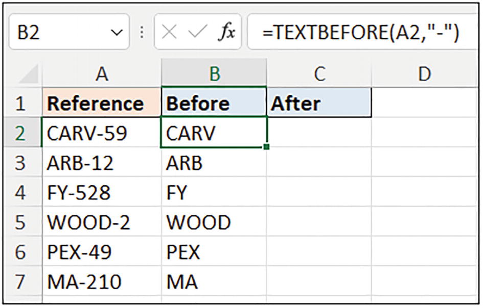
TEXTBEFORE to extract text before the first delimiter

TEXTAFTER to extract text after the first delimiter
Example 2: Specify an Instance Number
The instance number argument of the two functions is very useful when a delimiter occurs multiple times within a string. And both functions allow searching for the delimiter from the end of the string, in addition to a typical approach of searching from the start.
As shown earlier in this chapter, the SUBSTITUTE function can be used to help extract text before or after a specific instance of a delimiter. This is important for Excel versions without the TEXTBEFORE and TEXTAFTER functions.

TEXTAFTER the second instance of the delimiter

TEXTAFTER with instance number from the end of string
The ability to search from the end of the string made it simple to find the last occurrence of the delimiter and extract the web page from the URLs.
Example 3: Extract Text Between Two Characters
The TEXTBEFORE and TEXTAFTER functions can be combined to extract the text between two characters.

Extracting the text between two characters
In this example, the delimiter characters were unique. If they were duplicated within the string, the instance number argument could have been used.
Example 4: Using Match End and If Not Found
There are two different methods available with the TEXTBEFORE and TEXTAFTER functions to handle scenarios when the delimiter being searched is not found. They are the match end and if not found arguments.
Figure 5-47 shows a formula being used to extract a person’s name from a cell containing a person’s name and email address separated by a semicolon (;). The TEXTBEFORE function is used as the name occurs before the “;” delimiter.

Error returned when the delimiter is not found
Obviously, this is not ideal, and we would like the name to be returned despite the missing semicolon.

Using match end with TEXTBEFORE

Error returned when the second hyphen is missing
When the hyphen delimiter is missing, the end of the string can be used as an alternative delimiter. So, this is another example where the match end argument can be applied successfully.

Match end with TEXTBEFORE to ensure successful extraction
Keeping with this same data, we will use the TEXTAFTER function to extract the text after the second hyphen.

Error with TEXTAFTER due to missing delimiter

Match end applied with the TEXTAFTER function
Let’s imagine that the number after the second hyphen represents a version, and if the second hyphen does not exist, it means that it is the first version. So, instead of returning an empty string using the match end argument, we would prefer to return the value “1”.
In this scenario, using the if not found argument would be the better approach, as it allows us to return an alternative value.

If not found argument used to return an alternative value
The TEXTSPLIT Function
Availability: Excel for Microsoft 365, Excel for the Web, Excel for Microsoft 365 for Mac
Another new function released in 2022, and therefore only available on Microsoft 365 and the web versions of Excel, is TEXTSPLIT. This function has been eagerly anticipated by Excel users.
The TEXTSPLIT function splits text into multiple columns and/or rows at each instance of specified delimiters.
At its core, it is a formula alternative to the Text to Columns feature of Excel. The two are not directly comparable as they both contain some functionality that the other does not. But conceptually, it is the case.
TEXTSPLIT is an array function. The topic of dynamic arrays is not covered in detail until Chapter 10. However, it was logical to cover TEXTSPLIT at this point in the book. If you are not familiar with dynamic arrays in Excel, jump to Chapter 10 for a quick read through the basics.
Text: The text that you want to split.
Col delimiter: The character or text that determines where to split into columns. An array containing multiple delimiters can be used. This argument is optional. If omitted, a row delimiter must be provided.
[Row delimiter]: The character or text that determines where to split into rows. An array containing multiple delimiters can be used. If omitted, a column delimiter must be provided.
[Ignore empty]: Specify if you want to return a blank cell when two delimiters are consecutive. Enter FALSE to return the blank cell or TRUE to ignore the empty string and not return the blank cell. By default, the blank cell is returned.
[Match mode]: Specify if you want the delimiter match to be case-sensitive. Enter 0 for case-sensitive or 1 for case-insensitive. By default, a case-sensitive match is done.
[Pad with]: When data is missing, the #N/A error is returned to pad the cells that are missing data. Enter an alternative value to pad with to replace the #N/A error.
Example 1: Simple TEXTSPLIT

Simple TEXTSPLIT across columns with a single delimiter
Example 2: Using Multiple Column Delimiters
You can specify multiple column, or row, delimiters in the TEXTSPLIT function. The delimiters must be entered in an array.

Multiple column delimiters with TEXTSPLIT
In Figure 5-55, the TEXTSPLIT function returned an array of five columns. We only require four columns of values, but five were returned due to the consecutive delimiters of the closing bracket “)” followed by the hyphen “-” near the end of the string.
To prevent the blank cell from being returned, the ignore empty argument can be enabled within TEXTSPLIT.

Ignore empty option to prevent the creation of blank cells
Example 3: Splitting Across Rows (and Columns)
For the TEXTSPLIT function, you can enter either a column or row delimiter. You may even require both. Let’s see some examples of this.
In Figure 5-57, we have a cell that contains the details of four different people. For each person, we have a name and an email address.

Data to be split across rows and columns

Using the row delimiter with TEXTSPLIT
This nicely demonstrates that you are not required to specify a column delimiter; however, in this example we do want to split the name and email address into separate columns.

TEXTSPLIT with column and row delimiters specified
Example 4: Handling Missing Data

Error returned due to missing data
Using the pad with argument of TEXTSPLIT, we can return an alternative value to the #N/A error.

Empty string added for the pad with argument to suppress errors
Combine Text into One Cell
There are multiple functions in Excel that can be used to combine text from multiple ranges, arrays, or strings into one.
This has always been a popular task for Excel users, and with recent advances in the Excel function library and in how Excel handles arrays (Chapter 10), this has become easier and possibly in even higher demand.
Let’s have a look at the different functions to combine values into one cell – CONCATENATE, CONCAT, and TEXTJOIN – and how they differ from each other.
The CONCATENATE Function
Availability: All versions
The original function for combining cell values and strings into one is CONCATENATE. It is possibly the most well-known text function in Excel, and I still remember the day (many moons ago) when I first learned it.
In Excel 2019, CONCATENATE was replaced by a function named CONCAT. CONCAT can do everything CONCATENATE does, plus it can handle ranges of values, which CONCATENATE cannot.
When you enter CONCATENATE into a cell in a version of Excel 2016 or later, you see the compatibility sign next to its name (Figure 5-62).

CONCATENATE with compatibility sign

Combine multiple strings into one with CONCATENATE
To add delimiters between each part of the text, we will enter them as text enclosed in the double quotations.

Concatenate cell values with delimiters
Let’s see another example; this time, CONCATENATE is being used to change how a name is displayed. This demonstrates its flexibility.

Reverse names with CONCATENATE
For our final CONCATENATE example, we will see how to add line breaks into a text string. To do this, we will use the CHAR function with character code 10 – the line break character (character 13 on a Mac).
In Figure 5-66, we have a list of people and their top three preferred locations for something in columns L, M, and N.

Inserting line breaks with CHAR(10)
The Ampersand Character
Availability: All versions
An alternative to using the CONCATENATE function is to use the concatenate operator – the ampersand (&).

Reversing the names with the ampersand
You may have a preference as to whether you use the function or the operator. It is important to understand both, so that you can read and edit formulas that you inherit from other spreadsheet warriors.
The CONCAT Function
Availability: Excel 2016, Excel 2019, Excel 2021, Excel for Microsoft 365, Excel for the Web, Excel 2016 for Mac, Excel 2019 for Mac, Excel 2021 for Mac, Excel for Microsoft 365 for Mac
The CONCAT function was introduced in Excel 2016 to replace the CONCATENATE function. It works in the same way and with the added power of being able to work with ranges.
Text: The text or range of text values that you want to combine into a single text string

CONCAT function working with a range of values
This extra skill that CONCAT has over CONCATENATE can come in useful, but it cannot handle delimiters between the different text values of a range neatly. For that job, we will look at the TEXTJOIN function next.

CONCAT with delimiters
The TEXTJOIN Function
Availability: Excel 2019, Excel 2021, Excel for Microsoft 365, Excel for the Web, Excel 2019 for Mac, Excel 2021 for Mac, Excel for Microsoft 365 for Mac
The TEXTJOIN function was introduced in Excel 2019 and is a fantastic addition to Excel.
It enables us to specify a delimiter, can handle ranges of values, and has an option to ignore empty cells in a range. So, it contains some features that can make it more useful than CONCAT, although not as flexible.
One of the great strengths of TEXTJOIN is when working with spilled ranges. We discuss dynamic arrays and spilled ranges in detail Chapter 10, but we will see an example of TEXTJOIN and arrays soon.
Delimiter: The character to insert between the different text values.
Ignore empty: Would you like to ignore empty values. Enter TRUE to ignore the empty values and FALSE to include them in the resulting string. This is an optional argument, and if omitted, TRUE is applied to ignore the empty cells.
Text1, [text2]: The text or ranges of text values to be joined into a single text string.
TEXTJOIN and Delimiters
For the first TEXTJOIN example, we will use it to combine multiple values separated by the same delimiter.
We saw examples of CONCATENATE and CONCAT combine these same values earlier. With TEXTJOIN, the hyphen “-” delimiter needs only to be stated once, and the range of cells is used instead of individual cell referencing – a cleaner alternative to CONCAT.

TEXTJOIN handling delimiters with ease
TEXTJOIN and Empty Values
Let’s now see an example of the TEXTJOIN function ignoring empty values in a range that it is asked to combine.

TEXTJOIN function excluding empty values
Although it is not our objective in this example, let’s see what the results would look like if the empty values were included.

TEXTJOIN with empty values included
TEXTJOIN and Arrays
TEXTJOIN can combine the values from arrays with ease, which makes it especially useful in modern Excel.

Combine the offices for each continent into a single cell

Combining values from an array with TEXTJOIN
If you are using a version of Excel that is not Excel for Microsoft 365, Excel 2021, or Excel for the Web, you will need to press Ctrl + Shift + Enter to run the formula instead of just Enter.
This is an array formula, and handling arrays was only built into Excel after the 2019 version. Curly braces will be added around the formula if you press Ctrl + Shift + Enter.
The TEXT Function
Availability: All versions
The TEXT function is used to convert a value to text but apply a specific number format, such as a date in dd/mm/yyyy format, or display a text value as Euros with no decimal places.
This function is great for creating summary statements and other labels for your Excel reports and dashboards.
Value: The number that you want to format.
Format text: The number format enclosed in double quotes that you want to apply. The format code is similar to that used for number formatting in the Format Cells window.

Text formatted as a number using the TEXT function
The format codes used to format values with the TEXT function are similar to those used to format values in the Format Cells window. If these are new to you, it may be worthwhile familiarizing yourself with the commonly used symbols.

Format codes shown in the Format Cells window
Taking things up a notch from the previous example, the TEXT function is often given the result of a formula to format and is often combined with an ampersand or the CONCAT function to create a string of text.
Let’s see some examples of the TEXT function used in this manner and how it can be used to format different numeric values such as currencies and date formats.
Example 1: Currency Formats

Currency format applied to a text value
I live in the UK, so applying a format in pounds sterling is straightforward. If I need to apply a different currency format, I can utilize the tip I mentioned earlier and copy the format code from the Format Cells window.
- 1.
Open the Format Cells window and click Accounting in the Category list.
- 2.
Select € German (Germany) from the Symbol list and specify 0 decimal places (Figure 5-78).

Formatting values in a German Euros format
- 3.
Click Custom in the Category list and copy the format code from the Type field (Figure 5-79). In this example, I’m only copying the part of the code that is needed.

Copy the format code for the TEXT function
- 4.
Paste the copied format code into the required part of the TEXT function.

Using the format code in the TEXT function
There is a DOLLAR function in Excel that converts a number to text and applies the currency number format $#,##0.00_);($#,##0.00). The currency applied depends on your local language settings. So, for me, pounds sterling is applied when it is used.
The TEXT function offers much more than DOLLAR, so we will resign DOLLAR to a mention in this note, and no more.
Example 2: Positive and Negative Value Formats
When creating custom number format codes in Excel, positive, negative, zero, and text values can be displayed differently.
Each format is separated by a semicolon “;” when creating the format codes. Positive values are first, then negative values, then zero values, and finally text values.

Different formats for positive and negative values
Example 3: Date Formats

Formatting a date with the TEXT function
Date formats are easy to work with. You can change the number and order of the d’s, m’s, and y’s to get the format you want.
Text: “mm/dd/yyyy” Result: 03/27/2021
Text: “dd mmm yyyy” Result: 27 Mar 2021
Text: “ddd dd mmm yyyy” Result: Sat 27 Mar 2021
Text: “yyyy-mm-dd” Result: 2021-03-27
Repeating a Character – REPT Function
Availability: All versions
The REPT function repeats text a given number of times. It is often used to repeat a character in a cell.
Now this might not seem that useful, and you may be wondering why on earth someone would need to do this. That’s ok. I thought the same.
The REPT function is typically used to create in-cell charts that work nicely on your Excel reports. You can get creative with the different symbols and other characters in Excel to create some very nice visuals.
Text: The text to be repeated
Number times: The number of times to repeat the text
In Figure 5-83, the REPT function has been used to repeat the star symbol for the number of star ratings of each site.

Star rating system created with REPT
To insert the star symbol, it was first inserted to a cell on the worksheet from the Symbol window (Figure 5-84). Click Insert ➤ Symbol to access the Symbol window. This was then cut and pasted into the REPT function as shown before.

Insert the star symbol in Excel
Let’s see another example of using the REPT function to create in-cell charts. This time, we will create a simple bar chart to visualize the volume of upsells achieved by different sales representatives.
The cells containing the formula have been formatted using the Playbill font. This font looks great for these in-cell charts. The gray font color was also applied.

Creating in-cell charts using the REPT function
If the values to repeat are very large, for example, 1562, you do not want to repeat a character this many times in a cell. To work with this, divide each value by a consistent number. So, the 1562 and other values in that column could all be divided within the REPT function by 10.
Text Functions with Other Excel Features
Let’s see examples of how some of the text functions described in this chapter could be used with other Excel features.
Conditional Formatting Rules – Last Character Equals

Codes we want to apply the Conditional Formatting rule to
Conditional Formatting in Excel has a built-in “Text that Contains” rule. This can be useful for partial text matches.
- 1.
Select range A2:B7.
- 2.
Click Home ➤ Conditional Formatting ➤ New Rule ➤ Use a formula to determine which cells to format.
- 3.
Enter the following formula into the Format values where this formula is true: box (Figure 5-87):

RIGHT function in a Conditional Formatting rule
- 4.
Click Format and specify the formatting you want to apply.
- 5.
Click OK.

Conditional Formatting applied to the range
Data Validation Rules – Forcing Correct Case
For an example of text functions being used in Data Validation rules, we will validate the entry of region codes to always be in uppercase.
- 1.
Select the range that you want to apply the Data Validation rule to.
- 2.
Click Data ➤ Data Validation.
- 3.
Click the Settings tab of the window.
- 4.
Click the Allow drop-down and select Custom.
- 5.
Enter the following formula into the box provided (Figure 5-89):

EXACT and UPPER in a Data Validation rule
- 6.
Click the Error Alert tab and enter a meaningful Title and Error message to appear if a user enters a region code that is not in uppercase (Figure 5-90).
- 7.
Click OK.

Setting an error alert for a rule

Non-uppercase entries being prevented
Dynamic Labels for Charts
The TEXT function is fantastic for creating more meaningful labels on your Excel charts. You can go beyond the standard labeling used by many and provide more information to the readers.

Column chart with a chart title providing more information
There are two TEXT functions: one to display the revenue correctly and another for the percentage variance. The CHAR function is also used here to create the line break (character 10 for Windows and 13 for Mac).

Chart title created in a cell of the worksheet

Chart title linked to a cell for creative labeling
Typically, this formula would be hidden by entering it on a different sheet to the chart or in a hidden column. It is displayed here only to show the mechanics of the technique easier.
Summary
In this chapter, we covered the text functions of Excel, and, wow, there are many of them. These functions make it easy to extract, clean, split, combine, and convert text in Excel.
In the next chapter, it is time (sorry 😊) for the date and time functions in Excel. It is another extensive chapter, jam-packed with formula goodness.
You will first learn the fundamentals of dates and time in Excel. It is very important that this is understood to ensure correct and effective formulas with dates and times in Excel. The chapter then progresses through many functions, supported by many practical examples of their use.