
The introduction of dynamic array formulas in Excel is one of the greatest updates in Excel history. It completely changes the way that we think and write our formulas in Excel.
This fundamental change in how formulas calculate in Excel affects all formulas. So, this change can affect how you, or somebody else, write a classic Excel function such as SUM, IF, or VLOOKUP.
In addition to the introduction of the dynamic array formula engine, Microsoft released six new functions. These functions are commonly referred to as the dynamic array functions, though that is not an official function category.
Dynamic array formulas are only available in the Excel for Microsoft 365, Excel 2021, and Excel for the Web versions. When collaborating with Excel users from external organizations, you should exercise some caution, as they may have a different version of Excel to you.
In this chapter, we will begin by getting to know dynamic arrays. How do you use them, how would you recognize them on a spreadsheet, and what are their limitations?
We then go into detail on five of the six new dynamic array functions – UNIQUE, SORT, SORTBY, SEQUENCE, and RANDARRAY. The sixth function, FILTER, is covered on its own in Chapter 13.
Finally, we explore some examples of how the introduction of dynamic arrays has improved how we use existing Excel formulas. We focus on the FREQUENCY, TRANSPOSE, and SUM functions in this chapter, but the improvements go way beyond just those functions.
Getting to Know Dynamic Array Formulas
Availability: Excel for Microsoft 365, Excel for the Web, Excel 2021, Excel for Microsoft 365 for Mac, Excel 2021 for Mac
dynamic-arrays.xlsx
The formulas that we know and love in Excel have always been one cell, one formula. A formula would be filled, probably by clicking and dragging the fill handle, to any other cells in the range requiring that formula.
Dynamic arrays change all that. With the dynamic array formula engine, a formula can return multiple results. If a formula returns more than one value, the additional values are spilled to the adjacent cells. The range of cells that contain the formula is known as the spill range.
Notice the blue border surrounding the spill range. This appears when you click any cell within the spill range, making dynamic array formulas easy to identify on a spreadsheet.
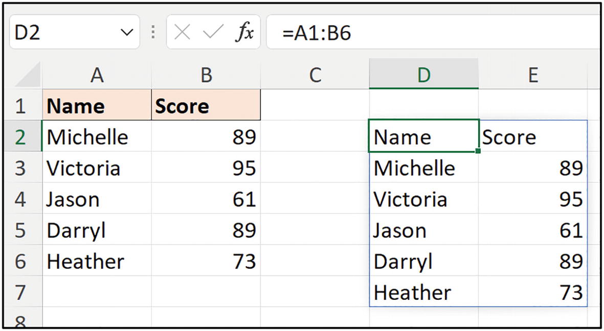
Dynamic array returning multiple values
- 1.
Select the output range D2:E7.
- 2.
Write the formula: =A1:B6.
- 3.
Press Ctrl + Shift + Enter.

Array formula in an Excel version without dynamic arrays
Array formulas were often referred to as CSE formulas due to the requirement to press Ctrl + Shift + Enter on running them.
The dynamic array formula back in Figure 10-1 only exists in the origin cell and spills the results (not the formula) to the other cells in the spill range.

Formula shown in spill range but is not present
Arrays vs. Dynamic Arrays
This example demonstrates nicely that although the use of arrays is not new in Excel, array formulas that output multiple results were awkward. You would need to know the cells that the formula would output to, which was a massive constraint to their use. They were static arrays.
So, dynamic arrays really are a combination of two key developments – dynamic + arrays.
These formulas are entered in the same way as any other formula and will handle arrays without the need to press Ctrl + Shift + Enter. And they are dynamic. You do not need to know the range of cells to output to. The spill range will dynamically grow and shrink depending on the number of values being returned by the formula.
Now, not all array formulas return multiple values, so single cell array formulas were easier to apply in the Excel of the past. You just needed to recall pressing Ctrl + Shift + Enter, and not just Enter.
However, did your colleagues know to press Ctrl + Shift + Enter, and what were the curly braces around the formula? Did you need to type them?
These limitations meant that, in the past, writing array formulas ended up being for advanced uses only, and the SUMPRODUCT function gained a lot of love as it could handle the arrays natively.
With dynamic array formulas, this is all a thing of the past.
Dynamic Arrays with Tables

Dynamic array formula referencing all values in a table
Using dynamic array formulas with table data is a dream combination. The first example that referenced range A1:B6 works great. However, it is not a fully dynamic solution as using the range as the source is not dynamic. So, you are losing 50% of the brilliant dynamic + array capabilities.
Tables are dynamic and grow and shrink with data automatically. So, using table data as the source for a dynamic array formula ensures a completely dynamic solution.

Dynamic array formula and table provide a fully dynamic solution
Dynamic Array Formula Example

Table of scores

Classic AVERAGEIFS being filled across other cells
With dynamic array formulas, we could reference the range of criteria values, instead of a single criteria value at a time.
Instead of producing three formulas – one formula per cell – the dynamic array formula is one formula that returns three results.

AVERAGEIFS returning a spill range
The output range of F3:F5 would need to be selected before writing the formula. No “spilling” in older versions.
The formula would exist in each cell, while dynamic arrays are one cell, multiple results.
The formula range would need to be in line with the range being referenced as implicit intersection would be applied. In this example, F3:F5 is in line with E3:E5 so it would work. The formula can be run as an array formula by pressing Ctrl + Shift + Enter to override the implicit intersection.
With dynamic arrays, none of this needs to be considered. The formula is written just like any other formula and wherever you want.
Implicit intersection is denoted by the @ symbol. In modern Excel, this is mainly seen in formulas in a table that reference other cells in the same row of a table, for example, =[@Country].
Welcome the # Operator
You may be wondering how one would reference the spill range of a dynamic array formula. You may want to use the results of a dynamic array formula in another formula or maybe in a chart.
If the spill range is dynamic, you wouldn’t necessarily know the final cell of the range.
Well, the answer, as I’m sure you have concluded from the title of this section, is the # symbol (typically referred to as the hash or pound sign).
To refer to all the cells in the spill range, you reference the origin cell that contains the dynamic array formula followed by the # symbol, for example, A2#.
The # symbol references the entire spill range including a spill range that contains multiple columns and rows. In Chapter 11, we will cover how the INDEX function can be used to reference specific columns or rows of a spill range only.

Spill operator accesses all values in a spill range
The #SPILL! Error
The #SPILL! error is created when the results of a dynamic array formula cannot be returned to the grid. This is typically caused by other content blocking the spill range.

#SPILL! error caused by content blocking the spill range
This is a similar behavior to what you may have encountered with PivotTables. They return an error when they are refreshed and need to expand in size but do not have the space to expand into.
The #SPILL! error is also returned if there are merged cells in the range that the formula needs to spill to or if a dynamic array formula is used within a table.
Figure 10-11 shows the #SPILL! error caused by merged cells in the spill range. The cells in range F5:G5 have been merged in this example.

Merged cells causing a #SPILL! error
Merged cells should only be applied in very specific cases in Excel. Very few actions can attract the ire of an Excel user more than the sight of merged cells.
DA Formulas Cannot Be Used Within Tables
The #SPILL! error is also caused by a dynamic array formula being used within a table. An example of this is shown in Figure 10-12. Note the blue corner in the bottom right indicating that the range is formatted as a table.

#SPILL! error caused by using a DA within a table
Let’s now look at the dynamic array functions that were released to take advantage of this new formula behavior.
UNIQUE Function
Availability: Excel for Microsoft 365, Excel for the Web, Excel 2021, Excel for Microsoft 365 for Mac, Excel 2021 for Mac
unique.xlsx
The UNIQUE function is a tremendous addition to Excel. It is incredibly helpful, and I find myself using it in most spreadsheets that I create.
Creating a distinct list of values is a very common Excel task. The Remove Duplicates button, the Advanced Filter, and PivotTables are popular tools to generate a distinct list of values in Excel. This distinct list may be used as the source for a Data Validation list or to create labels for a report.
This function is often used as a formula alternative for creating a distinct list of values. Being a dynamic array function, this approach would ensure a dynamic list that updates when values are added, removed, or changed in the source data.
In addition to returning a distinct list of values, this function can also return a unique list of values (as its name implies). We will cover the distinction (pun fully intended) between the often misunderstood terms of distinct and unique shortly.
Array: The range or array from which to return the values.
[By col]: To compare the values in rows or columns. Entered as a logical value (True/False). The default is FALSE to compare values in rows. Enter TRUE to compare the values in columns.
[Exactly once]: A logical value. The default is FALSE to return a distinct list of values. Enter TRUE to return a list of the unique values (those that only occur once).
Returning Distinct and Unique Values
The UNIQUE function, despite its name, actually returns the distinct values by default. A list of the distinct values is a list with the duplicate values removed. This is the most common use of this function.
A list of the unique values is a list of values that occur only once in the list. This is specified by entering TRUE for the final argument of the UNIQUE function.
There is a lot of confusion over the terms distinct and unique. Users often refer to a list of distinct values as a list of unique values. So be prepared for that when conversing with other Excel users.
It does not help that Microsoft named the function UNIQUE, yet it returns a distinct list by default. I believe it was named UNIQUE as that is the more common term, and Excel users would be more familiar with it. The final argument does however coincide with the function name. Enter TRUE for a unique list, or enter FALSE or omit the response for a distinct list.

Distinct list of values returned by UNIQUE
Remember that these dynamic array functions automatically update as the source data changes. This formula has a table source for a dynamically complete formula.

Returning unique values with the UNIQUE function
UNIQUE with Multiple Columns
The examples so far have demonstrated the UNIQUE function with a single column. However, UNIQUE can handle multicolumn arrays or even entire tables as the array from which to return the distinct or unique results.

UNIQUE function using a multiple column array
In this multiple column array example, the columns were adjacent. In fact, the formula used the range tblPoints[[Name]:[Office]].
Let’s see how the UNIQUE function can be used with a multiple column array where the columns are non-adjacent.

Returning non-adjacent columns with UNIQUE
UNIQUE to Compare Columns
The UNIQUE function compares the values in rows by default. This is the more common practice as we handle columnar data usually.
It is no problem for UNIQUE to work with data stored in rows though, if required. The second argument of the UNIQUE function allows us to switch to comparing values in columns. This is done by entering TRUE for the second argument named By col.

UNIQUE function comparing columns
The results are returned along a row. The TRANSPOSE function could be used to convert the results into a column. This example is shown when we cover TRANSPOSE later in the chapter.
Distinct Labels for SUMIFS
We covered an example earlier in the chapter that used the AVERAGEIFS function on a range of criteria values. This generated a spill range with the results for each criterion in that range (Figure 10-8).
That example was a static report as the criteria values were simply typed into the cells. Let’s explore a dynamic solution where the UNIQUE function will return the distinct values from a table. A SUMIFS function will then use the spill range generated by UNIQUE for its criteria values.

Table of sales data

Table showing sales by product using UNIQUE and SUMIFS
Distinct Count Formula
The examples so far have all returned values to the grid. The UNIQUE function can, of course, also be nested within other functions. A natural example of this would be to count the number of distinct values returned.
In Chapter 9, we created a distinct count formula using SUMPRODUCT and COUNTIFS. With dynamic arrays and the UNIQUE function, this is much simpler.

Count distinct and count unique formulas
SORT Function
Availability: Excel for Microsoft 365, Excel for the Web, Excel 2021, Excel for Microsoft 365 for Mac, Excel 2021 for Mac
sort.xlsx
Sorting the data in a table is one of the most common everyday tasks that an Excel user performs. The introduction of the SORT function to automate the sorting of the data is a revelation for how we create in Excel.
In the past, PivotTables, VBA, or an overly complex formula would be used to automate the sorting of data in Excel reports and models. With the SORT function, this is now very easy to do.
Array: The range or array of data that you want to sort and return.
[Sort index]: An index number that represents the column or row of the array to sort by. If omitted, the first column or row of the array is used.
[Sort order]: The order that the column or row should be sorted. Enter 1 to sort in ascending order and –1 to sort in descending order. If omitted, it will sort in ascending order.
[By col]: A logical value that specifies whether to sort by row or by column. The default value is FALSE, which sorts by row (vertical sort). Enter TRUE to sort by column (horizontal sort).
Simple SORT Example
Let’s start with a simple example of the SORT function being used to sort a single column of data.
In Figure 10-21, the following formula sorts the list of country names in ascending order.

Simple example of the SORT function
Sort the Distinct Values

Total sales by product in no particular order
The results in this report are in no particular order. They actually appear in the order that UNIQUE finds them in [tblSales]. This is not useful. Let’s use the SORT function to sort the distinct list of product names in ascending order.

Sorting the values returned by UNIQUE
Sort by Specified Column

Table of product sales

SORT function returning a multiple column array
Let’s specify a different column for the results to be sorted by. We want the results to be in a descending order by the [Total] column.
We need to provide the SORT function with the sort index. So, for the [Total] column, this will be column 4.

SORT results by column 4 in descending order
Sort by Multiple Columns
It is possible to request the SORT function to sort using multiple columns. To do this, we will enter the multiple sort indexes and sort orders within arrays.
For this example, we will sort the [tblProductSales] data by two levels: first by the [Category] column in ascending order and then by the [Total] column in descending order.
The array {2,4} is used in the sort index argument to specify that the data should be sorted by column 2 and then by column 4.
The array {1,-1} is used in the sort order argument to state that column 2 should be sorted in an ascending order and column 4 should be sorted in a descending order.

Sorting an array by multiple columns with SORT
SORT Function Returning Specific Columns from a Table
For the final SORT function example, we will return specific columns from [tblProductSales].
Dynamic array functions in isolation can only return columns that are adjacent to each other. In this example, we will return the [Product Name], [Units], and [Total] columns only.
These columns are split by the [Category] column in the table, so SORT will need some assistance to work with these columns as they are non-adjacent.
To do this, we will nest the CHOOSE function within the SORT function to specify the columns to work with. We saw the CHOOSE function assuming this role previously in this chapter within the UNIQUE function.
In Chapter 11, we will see the INDEX and MATCH functions together to create a more dynamic method for returning non-adjacent columns in dynamic arrays.

SORT function returning specific columns from a table
When returning only three columns, this works quite well and is simple to deploy. In more complex examples, this CHOOSE technique can be bulky, and a more advanced technique would involve the INDEX function. We will see examples of this technique in Chapters 11 and 13 of the book.
No examples are shown in this chapter of sorting data by column (sorting horizontally) due to the rarity of this behavior. Excel data is better in a columnar layout. However, TRUE can be entered for the By col argument to sort horizontally. An example of the By col argument was shown with the UNIQUE function previously.
SORTBY Function
Availability: Excel for Microsoft 365, Excel for the Web, Excel 2021, Excel for Microsoft 365 for Mac, Excel 2021 for Mac
sortby.xlsx
If the SORT function is not enough for you, Microsoft also gave us SORTBY. There are benefits for using each of these two sort functions.
The SORT function is perfect for very simple single column sorting. It is also better for sorting based on dynamic columns, as the columns are specified using index numbers.
The column to sort by is specified using the range or array. This absolute reference to the column to sort by makes it fantastic for use with table data.
With the SORTBY function, you can sort an array by a column that is outside of the array being returned.
Array: The range or array of data that you want to sort and return.
By array1: The range or array to sort by. The array must be one column wide or one row high.
[Sort order1]: The order that the column or row should be sorted. Enter 1 to sort in ascending order and –1 to sort in descending order. If omitted, it will sort in ascending order.
[By array2], [sort order2]: The corresponding arrays to sort by and sort orders for any additional sort levels you require.
Note The SORTBY function can sort data that is arranged in rows or columns. It does not have a special argument for this functionality like UNIQUE and SORT do. SORTBY will automatically understand the direction of the sort and spill range.
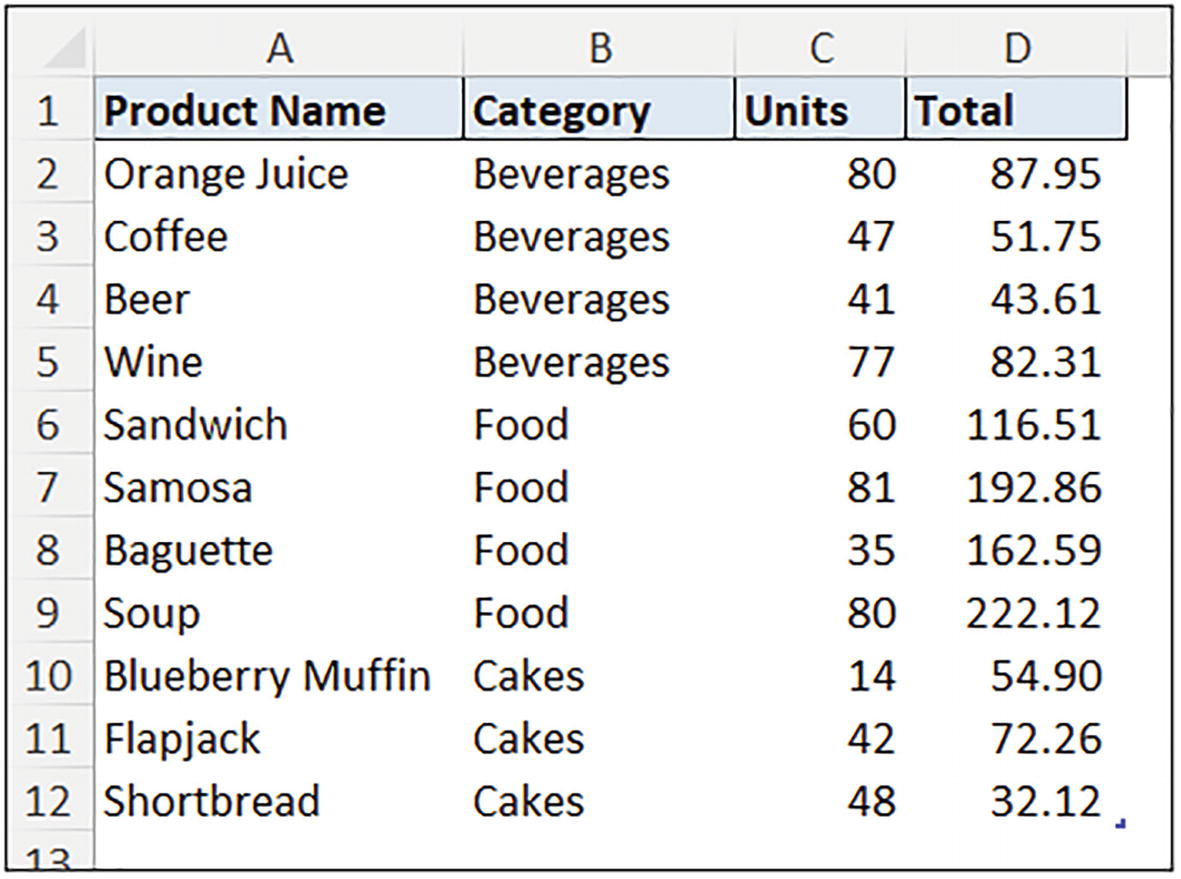
Table of product sales
Simple SORTBY Example
Let’s begin with a simple example that returns all columns from the [tblProductSales] table sorted in descending order by the [Total] column.

Simple SORTBY example sorting the array by the [Total] column
Sort by Multiple Columns with SORTBY
The SORTBY function can sort an array by multiple columns, and, once again, it is an easier task than the equivalent formula with the SORT function (Figure 10-27).
SORTBY has arguments for us to keep specifying the additional columns and sort orders that we want to apply.

Sort by multiple columns with SORTBY
Sort by Column Outside of the Returned Array
A great advantage that the SORTBY function has over SORT is the ability to sort an array using a column, or row, that is not included in the returned array.

SORTBY sorting by a column not included in the returned array
This can be a very useful technique. Let’s see another example.
Sort Product Name by Sales Totals

Sales by product sorted by the product name
We will change this to sort the results by the total sales in a descending order. It will be more practical to order the products by the sales total rather than their name. And it’s a great example of how useful SORTBY is.
We will start by using the SORTBY function to sort the product names by the sales totals. The SUMIFS function will be used to sum the [Total] column for each product. With the product names ordered correctly, the SUMIFS function will then be used again to create the column of total sales values.

Sort product names by sales totals in descending order
This is another nice example of using SORTBY to sort by an array outside of the one being ordered. We now need to return the totals.

SUMIFS to sum the totals for each product
SEQUENCE Function
Availability: Excel for Microsoft 365, Excel for the Web, Excel 2021, Excel for Microsoft 365 for Mac, Excel 2021 for Mac
sequence.xlsx
The first time that you see it, it may not immediately be apparent how brilliant the SEQUENCE function is. Certainly not in the way that functions such as SORT and UNIQUE will instantly earn your affection. But believe me, SEQUENCE is an awesome function.
The SEQUENCE function returns a series of numbers. It is the formula equivalent of the Fill Series feature in Excel. As a function, we can nest it within other functions to create some real formula magic.
Rows: The number of rows to return.
[Columns]: The number of columns to return.
[Start]: The first number in the sequence. If omitted, the sequence begins from one.
[step]: The amount to increment each subsequent value in the sequence. If omitted, it will step one at a time.
Stepping into the SEQUENCE Function
Let’s start with some basic examples to get a feel for how to operate the SEQUENCE function. This will prepare us for the more practical examples to come in this chapter and the next.

Number series across rows with SEQUENCE

Using the rows and columns arguments of SEQUENCE

SEQUENCE function with all arguments specified

Reversing a sequence with a negative step
In this example, the columns argument is skipped. The default one column wide is used.
Changing the Row/Column Order
When returning a two-dimensional array, we saw that the numbering of the series goes across columns, before going to the next row (Figure 10-38).
To switch the ordering of the numbers in the series, the TRANSPOSE function could be wrapped around SEQUENCE.

Changing the row/column order with TRANSPOSE
Let’s see some examples now that really showcase the flexibility and potential of the SEQUENCE function.
Sum the Top N Values
Performing a calculation on the top N values is a common task for reporting in Excel. For this example, we will sum the top N values, but a calculation such as average could also be applied.
We saw a method to sum the top five values in Chapter 9 with the SUMPRODUCT function. This was great as it works for all versions of Excel.
If you have a dynamic array–enabled version of Excel though, there is a better way. It is simpler and more dynamic. And of course, SEQUENCE plays an important role.
The LARGE function will also be used in our formula. This function has been covered already in this book, but let’s briefly remind ourselves of the purpose and syntax of the LARGE function.
Array: The range, table column, or array from which to return the kth largest value
K: The position of the value in the array (from the largest) that you want to return
The SEQUENCE function is used for the K argument of the LARGE function. It returns an array of numbers determined by the value in cell D3. In this example, cell D3 contains the number 3, so the SEQUENCE function returns {1,2,3}.
This replaces the need to enter an array of constants like we did in the SUMPRODUCT example in Chapter 9. This also keeps it dynamic.

Summing the top N values
Sum the Last N Days
The SEQUENCE function is great for creating a series of dates that occur at specific intervals. The activity on these dates can then be analyzed with other formulas or charted.
For this example, we will use the SEQUENCE function to return the last N days. We will find the last date in a range and then return each date for the last N days. The number of days will be specified by a cell value.

tblSales data with daily transactions
This is a fully dynamic solution.

SEQUENCE returning a series of dates for analysis
Sum the Last N Months
Let’s expand on this example and get the SEQUENCE function to return the last N months from the last month in the [tblSales] table.
The DATE function is used to construct a date value for the results. These values could be formatted to show month names using the custom number formatting feature of Excel. I have not bothered with this in the example, as I’m happy to show the first date of each month.

DATE and SEQUENCE functions to return last N months
The spill range is accessed using E5# for the first date of the month.
The EOMONTH function is used to return the last date of a month a specified number of months in the future or past. A zero is entered for the months argument to return the last date of the current month.

Total values between first and last day of a month
The DATE and EOMONTH functions were covered in detail in Chapter 6.
Last N Months by Country – Pivot Style Report
The last two examples have used the SEQUENCE function to spill the date values across rows. But, of course, SEQUENCE can spill across columns also. This feature can be used to create awesome pivot style reports with time-based analysis.
There are some differences in this formula compared to the previous one that spilled across rows.

SEQUENCE for last N months spilled across columns
Sum Values from Alternate Rows/Columns
There are many scenarios in Excel where we can take advantage of the SEQUENCE function and its ability to return a sequence of values. Another of these scenarios is to perform a calculation on the values in every Nth cell. In the first of these examples, we will sum the values in alternate rows.

Sum alternate rows with SEQUENCE
Four numbers are returned, as the ROWS function returns the total number of rows in the table (eight), and this is divided by two as we want every other row, that is, half the rows.
The ROUNDUP function is included in the scenario that we have an odd number of rows. In this example, it is not relevant, as we are dealing with income and expenses, so the total rows will be an even number. However, it has been added for completeness. If there were 9 rows in total, half would produce 4.5 and ROUNDUP would make this 5. The rows {1;3;5;7;9} would be returned in that scenario.
The columns and start arguments are omitted, and the SEQUENCE function is asked to step by two.
With the SEQUENCE function, the values that we step through can represent rows or columns, and we can specify any Nth value. For a second example, we will return to a task that we completed with the SUMPRODUCT function along with others in Chapter 9.

Summing the value in every Nth column
This time, the rows argument is omitted, and the COLUMNS function is used to return the total columns in the range C2:J2 (eight columns). This value is then divided by four (the number of columns we want to step) to return the result of two columns.
The INDEX function then returns the values from columns 4 and 8 in the range C2:J2 to be summed. Notice that the rows argument of INDEX is omitted.
We will see more of the INDEX and SEQUENCE functions working together when we discuss the INDEX function in detail in Chapter 11.
RANDARRAY Function
Availability: Excel for Microsoft 365, Excel for the Web, Excel 2021, Excel for Microsoft 365 for Mac, Excel 2021 for Mac
randarray.xlsx
For years, Excel has had two functions that are used to return random values – RAND and RANDBETWEEN. There is now a third musketeer – the RANDARRAY function. This function merges the characteristics of the two existing functions along with further advantages.
RAND and RANDBETWEEN
Availability: All versions
Let’s begin with a quick look at the RAND and RANDBETWEEN functions. They are still great to use, and understanding them will help us appreciate the role that RANDARRAY plays.

RAND function generating random numbers between 0 and 1
Bottom: The smallest integer number that RANDBETWEEN can return
Top: The largest integer number that RANDBETWEEN can return
It has been entered in cell B2 and filled down five rows and across three columns to cell D6. There are 15 formulas entered to produce these random values. It is probably no surprise that RANDARRAY can handle this task also with just one formula that spills.
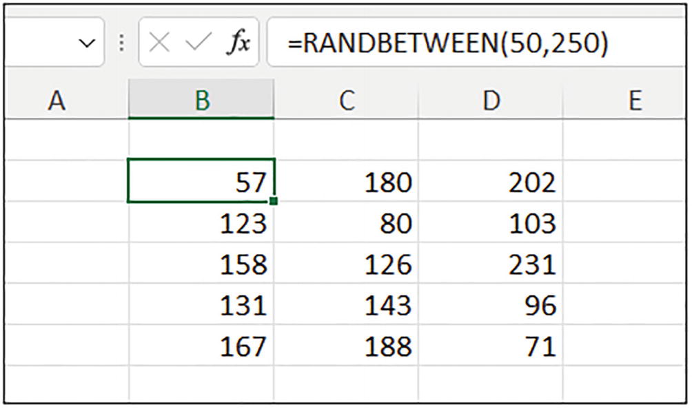
RANDBETWEEN returning random integer numbers between 50 and 250
Both functions generate a new random number every time the worksheet calculates.
Functions that behave in this manner are known as volatile functions.
Introduction to RANDARRAY
The RANDARRAY function returns an array of random numbers. All the finest qualities of RAND and RANDBETWEEN are included, with the added ability to return a dynamic array that spills.
You can specify the number of rows and columns to spill, whether you want decimal values or integers, and you can specify the bottom and top values from which to return the random number(s).
[Rows]: The number of rows to return.
[Columns]: The number of columns to return.
[Min]: The smallest number that the RANDARRAY function can return.
[Max]: The largest number that the RANDARRAY function can return.
[Integer]: Would you like an integer value returned? Type TRUE to return an integer value or FALSE for a decimal value. If omitted, FALSE is applied and decimal values are returned.
Let’s look at a few examples that show different applications of these arguments. Then we will see two practical examples of RANDARRAY.

RANDARRAY with no arguments entered
And in Figure 10-52, the RANDARRAY function returns a random integer number between 5 and 250. It is behaving like RANDBETWEEN in this example.

RANDARRAY being applied like RANDBETWEEN
Now, these examples show us nothing that we could not have achieved with the existing RAND and RANDBETWEEN functions. They are only shown to provide an extensive understanding of using RANDARRAY and to show that the characteristics of both existing random number–generating functions exist within RANDARRAY.
A key advantage of RANDARRAY is clearly its ability to return an array and therefore be used within our dynamic array formulas.
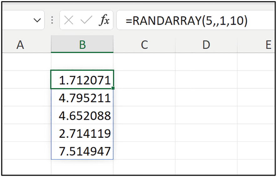
RANDARRAY returning five rows of decimal values between 1 and 10
This example not only demonstrates an array being returned but also RANDARRAY returning decimal values larger than 1. This is something that the RAND and RANDBETWEEN functions alone do not offer. RANDBETWEEN returns integers only, and RAND returns decimal values, but only between 0 and 1.

RANDARRAY with all arguments completed
Pick a Name from a List at Random
A practical example of using the RANDARRAY function is to return a value at random from a list. In this example, we want to return a name at random from a table named [tblNames].
The random value returned by RANDARRAY is used as the row number to return the name from. This is the row of the table, not the row of the spreadsheet. The INDEX function is used to return the name from that row of the [tblNames] table.

Returning a name at random from a list
A different name is returned every time the worksheet calculates. The F9 key is pressed to run calculations on the worksheet.
Shuffle a List of Names
In this example, we will shuffle a list of names, changing the order every time the sheet is calculated. This is a solid example of dynamic arrays in action, as we are now returning an array that is dynamic.
The RANDARRAY function has been inserted into the by array argument of the SORTBY function. So, the names are sorted by randomly generated numbers.

Using RANDARRAY and SORTBY to shuffle a list
An example of the RANDARRAY function is shown with the CHOOSE function in the next chapter to randomly generate some sample data. This is useful for testing and practice.
FREQUENCY and TRANSPOSE Functions
Availability: All versions
frequency-and-transpose.xlsx
Dynamic array formulas are not all about the fabulous new functions. Existing Excel functions also benefit from the array engine. Two functions that really saw a new lease of life were the FREQUENCY and TRANSPOSE functions.
These two functions are array functions. So, in older versions of Excel, they were very awkward to use. The output range had to be selected before writing the formula, and then the user would have to press Ctrl + Alt + Enter to run the function.
With the dynamic array formula engine, these functions are just like any other Excel function. They have essentially been reborn.
FREQUENCY Function
The FREQUENCY function calculates how often values occur within a range of values (known as bins). The results are always returned as a vertical array.
Data array: The range, array, or table column that contains the values for which you want to count the frequencies.
Bins array: The range or array that contains the intervals for which to group the values.
The score must be greater than the interval value to be grouped in that range. So, the bins array can be read as 1–50, 51–65, 66–80, 81–90, and >90.
The FREQUENCY function always returns one extra value to the number of intervals in the bins array. This extra value is the count of values greater than the largest interval.

FREQUENCY function returning the frequencies of scores
In Chapter 8, we saw the COUNTIFS function used to create a frequency distribution table. This is my preferred approach due to the extra flexibility it provides. However, FREQUENCY is great and was built for this purpose.
TRANSPOSE Function
Not many functions benefitted from the introduction of the dynamic array engine more than TRANSPOSE. The TRANSPOSE function was a sleeping giant shackled by Excel’s inability to natively handle arrays in older versions.
The shackles have now been broken for this function to show its value. Welcome to TRANSPOSE 2.0.
Many people are familiar with the transpose functionality that is available when you copy and paste data. This is very useful. With the TRANSPOSE function, you can automatically transpose the results of a formula or feed a formula with a transposed array.

Switching horizontal data to vertical with TRANSPOSE
In versions of Excel that do not have dynamic arrays, the TRANSPOSE function is a horrible experience.
To achieve the same result for this example, you would need to select the output cells for the TRANSPOSE function. The range to be transposed is seven columns wide and three rows high. So, you would need to select an output range that is three columns wide and seven rows high and then type the TRANSPOSE function followed by pressing Ctrl + Shift + Enter.
This is not a feasible way to work. It is awkward, not dynamic, and required Ctrl + Shift + Enter to operate.
Thankfully, it now works like any formula – one cell, one formula that spills.
Let’s see a quick second example.
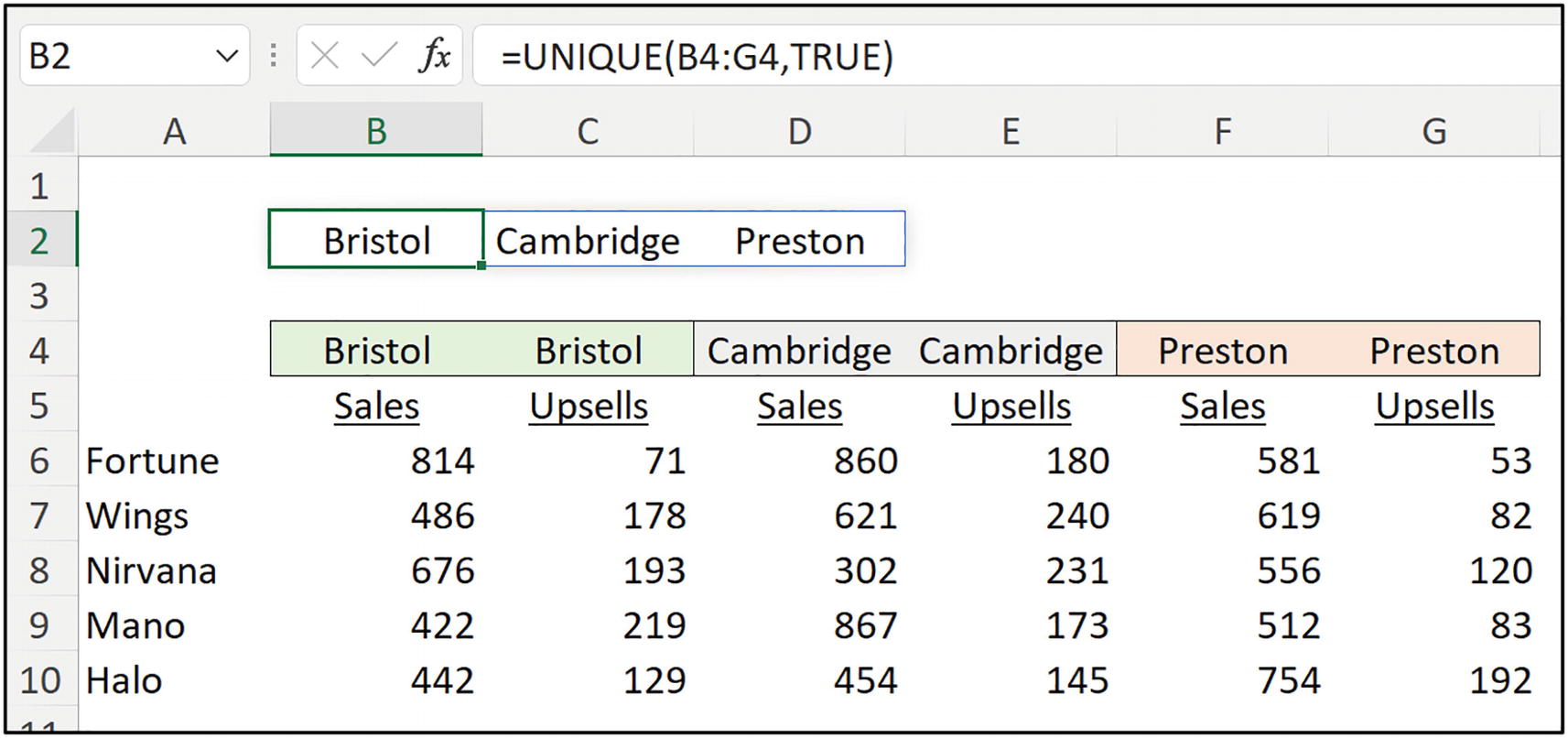
Data containing duplicate values in range B4:G4
We may need this array to be rotated into a vertical array. This could be to feed a Data Validation list or maybe to feed an Excel function that only works with vertical arrays (there are a few).

Transposing a horizontal array returned by UNIQUE
The TRANSPOSE function was shown with the SEQUENCE function earlier in this chapter to change the column-row order that SEQUENCE uses when producing two-dimensional arrays.
PivotTable Style Report Using Formulas
A fantastic use of the TRANSPOSE function is how it can be used to produce labels for a PivotTable style report.
We saw an example earlier in the chapter of the SEQUENCE function generating time-series data across columns for a PivotTable style report. This is simple with SEQUENCE as it has a columns argument, and this is great for numeric values. But to get text values dynamically displayed across columns, TRANSPOSE is superb.

Sales data to be used as the source for a pivot style report
We will create a report that displays the [Product Name] values as row labels and the [Store] values as column labels. To show the [Store] values across columns, they will need to be transposed. The values in the [Total] column will be summed for each product and store.

TRANSPOSE for column labels in a pivot style report
This is the reverse of the previous two examples where the TRANSPOSE function was used to switch data that was arranged horizontally to vertically.
By using dynamic array formulas based on a table, we have a completely dynamic solution here that updates automatically, unlike PivotTables. It also provides greater flexibility than a built-in tool like PivotTables would allow.
SUM v2.0 – The DA Version
Availability: Excel for Microsoft 365, Excel for the Web, Excel 2021, Excel for Microsoft 365 for Mac, Excel 2021 for Mac
sum.xlsx
Excel’s number one function, the SUM function, has also had a new lease of life thanks to the array engine available in Excel 365, Online, and 2021.
In modern versions of Excel, a simple SUM can perform the tasks that we would previously rely on SUMPRODUCT for. It can handle complex arrays, multiple conditional sums, and multiple columns of values (unlike SUMIFS).
Let’s welcome SUM 2.0.
Sum Based on Complex Criteria
Let’s dive straight in and see the SUM function performing a sum that is based on complex criteria. We need to perform both AND and OR logic in the criteria of this formula.

Table of sales data

SUM based on complex criteria including AND and OR logic
When performing formulas such as this, the “+” operator is used to stipulate OR logic between conditions, and the “*” specifies AND logic. An extra set of brackets surround the OR logic part of the formula to force that operation to calculate before the AND operation.
We saw this example in Chapter 9 when we covered the SUMPRODUCT function in detail. In modern Excel, SUMPRODUCT is no longer required for this work. For a detailed breakdown of how this formula works, visit the “SUMPRODUCT Function” section of Chapter 9.
In Chapter 8, we saw a neat trick to combine the SUM function with the SUMIFS and COUNTIFS functions for a more dynamic version of a formula like this.
Sum with Arrays
As formulas in Excel can now handle arrays, this reduces the requirement for using intermediary formulas that store their results in columns.
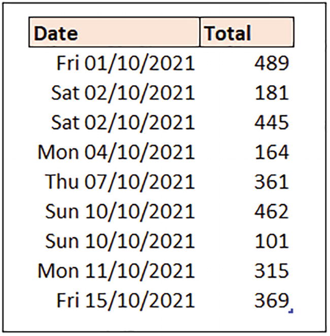
Table with daily transaction
In non-dynamic array–enabled versions of Excel, the typical approach would be to use the WEEKDAY function in a column to return the number that identifies the day of the week. A function such as SUMIFS can then be used that tests the values from the weekday column to sum the required values.
The WEEKDAY function returns a number that identifies the day of the week. The week starts from a Monday as 1 and ends with Sunday as 7. The formula tests if the value returned by the WEEKDAY function is greater than 4.
The results of this logical expression are multiplied by the values in the [Total] column and then summed by the SUM function.

Summing the sales from Friday to Sunday
Sum Based on Multiple Columns
The SUM function is extremely versatile and can sum values of any array dimensions and include any criteria.

Sales matrix by product and location

Summing values from multiple columns
Taking it a step further, we can set both row and column criteria, creating a two-way SUM.

Two-way SUM with row and column criteria
Although this section of the chapter is dedicated to SUM, it is worth noting that all aggregation functions benefit from the array engine. We have seen other examples in this book that showcase this, for example, the conditional median function using MEDIAN and IF shown in Chapter 8.
Dynamic Array Formulas with Other Excel Features
Dynamic array formulas have a mixed relationship with other Excel features. Some features work well with DA formulas, although we may need to reference them indirectly, while others do not recognize DA formulas at all.
Let’s look at how DA formulas can be used in combination with Conditional Formatting rules, Data Validation rules, and charts in Excel.
DA Formulas with Conditional Formatting
Unfortunately, Conditional Formatting does not recognize a spill range. You cannot reference a spill range directly in a Conditional Formatting rule. And if you select a spill range and apply a Conditional Formatting rule to it, it will not update dynamically with the spill range.
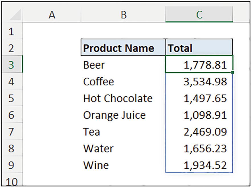
Spilled range in range C3
We will apply a Conditional Formatting rule to change the cell color for all values that are greater than or equal to 1700.
The approach we will take to make the best of an unfortunate situation is to select more cells than is required. The dynamic array formula may expand the spill range in the future, and we want the rule to apply to the additional cells.
As mentioned, Conditional Formatting cannot work directly with a spill range, so we must resort to selecting cells on the grid and plan a little for future changes.

Selecting additional cells beyond the spill range
- 1.
Click Home ➤ Conditional Formatting ➤ New Rule.
- 2.
Click Format only cells that contain.
- 3.
Select greater than or equal to from the list of logical operations and type “1700” into the box provided (Figure 10-72).
- 4.
Click Format and specify the formatting you want to apply.
- 5.
Click OK.

Format cells greater than or equal to 1700
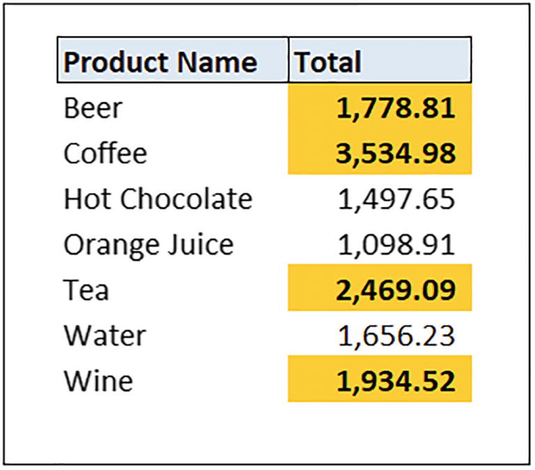
Conditional Formatting rule applied
DA Formulas with Data Validation
The good news is that Data Validation works with dynamic array formulas. You cannot enter DA formulas directly in the Data Validation window, but you can reference spill ranges on the grid. When the spill range updates, the Data Validation rule will update with it.

Table with subscriber data
We will create a dynamic Data Validation list from the countries in the [Country] column. If subscribers are added from new countries, the Data Validation list will automatically update to include them.

Spill range to be used as the source for a DV list
- 1.
Click the cell(s) you want the Data Validation list in.
- 2.
Click Data ➤ Data Validation.
- 3.
From the Settings tab, click the Allow list and click List.
- 4.
Click in the Source box, click the cell that contains the spill range, and type the # operator after the reference (Figure 10-76). The following reference is used in this example. Click OK.
A defined name could be created for this reference, such as lstCountries, and then the defined name used for the source of the Data Validation rule. This is not required but is a nice technique for a more meaningful reference than $B$3#, especially if the spill range was on another sheet.

Data Validation list referencing a spill range

A dynamic Data Validation list of countries
DA Formulas with Charts
It is further good news for charts in Excel, as they also can be used with dynamic arrays. When the spill range of a dynamic array updates, the chart will update with it.
However, the spill reference cannot be used directly in charts. Also, if a chart is created by selecting the spill range on the grid, it does not update with the spill range.
We need to define a name for each spill range and then use the defined name in the appropriate areas of the chart.

Spill ranges for products sorted by sales totals
This is a cool technique, and we demonstrated how to create this report earlier in the chapter with the SORTBY function.
We will insert a column chart that is connected to these spill ranges, so that the chart always sorts the product names by their sales totals in descending order.
- 1.
Click cell B3.
- 2.
Click Formulas ➤ Define Name.
- 3.
Type a Name for the defined name. In Figure 10-79, “rngProducts” is used.
- 4.
The reference to cell B3 should automatically appear in the Refers to box, as we clicked the cell before defining the name. Add the # operator to the end of the reference. Click OK.

Define a name for the product name’s spill range
- 5.
Click cell C3 and repeat the previous steps using the following reference. In this example, the name “rngSalesTotals” is used for the defined name.
- 6.
Click Insert ➤ Insert Column or Bar Chart ➤ Clustered Column.
- 7.
With the chart selected, click Chart Design ➤ Select Data.
- 8.
Click the Add button in the Legend Entries (Series) area on the left.
- 9.
Type “Product Sales” for the Series name and type the following reference in the Series values box (Figure 10-80). Click OK.

Editing the series for a chart to use the defined name
Even though the defined name has workbook scope, it is essential that the references in charts include the sheet name.
Instead of typing the defined name into the field, you can also press F3 to open the Paste Name window and select it from there.
- 10.
Click the Edit button in the Horizontal (Category) Axis Labels area on the right.
- 11.
Type the following reference into the Axis label range box and click OK (Figure 10-81).

Editing the axis labels to use the defined name
- 12.
Click OK to close the Select Data Source window.

Completed chart using dynamic array sources
Summary
Understanding what exactly a dynamic array is and how to use them effectively in Excel.
Learning a few of the dynamic array functions in Excel including SORTBY, UNIQUE, and SEQUENCE. Others such as TEXTSPLIT, FILTER, and STOCKHISTORY are covered in other chapters of the book.
How existing functions in Excel such as SUM, TRANSPOSE, EOMONTH, and SUMIFS work with arrays. Functions such as SUM are better than ever, while EOMONTH requires some tricks to work effectively.
How dynamic array are used with existing features of Excel such as charts and Data Validation.
In the next chapter, we will dive deeper into the lookup functions of Excel. We have covered VLOOKUP in this book already, but there are many more (and better) lookup functions in Excel than VLOOKUP.
We will cover functions including INDEX, CHOOSE, OFFSET, VSTACK, and INDIRECT. It is the largest chapter of this book, containing many examples and pro tips.