
It is almost inevitable that you will work with dates and time in Excel, regardless of your job role or profession. Excel contains more than 20 awesome functions for you to perform the date and time calculations that you need.
This chapter begins with a guide to how dates and time work in Excel. It is very important that we understand the calendar system of Excel before we begin writing our formulas.
We then proceed into explanations of the most used date and time functions with examples using them to solve a myriad of typical business tasks.
I am based in the UK, so all dates shown are entered in a dd/mm/yyyy format unless specified otherwise. I will often refer to dates using the month name, for example, 1st September 2021, to avoid any confusion with translation.
Understanding Dates and Time
dates-and-time.xlsx
Working with dates and time in Excel can certainly get interesting. To effectively work with the formulas of Excel, we must first understand how dates and time are stored.
Dates and the Calendar System in Excel

Serial number mentioned in the WORKDAY function description
When a date is entered into Excel, it is converted to a serial number based on the 1900 date system and formatted as a date. The 1900 date system begins on 1st January 1900. For Excel, this is the beginning of time. All dates are a sequential number beginning from this date.

The serial number of dates shown in Excel
Excel actually supports two different date systems, the 1900 date system and 1904 date system. The 1904 date system starts on 1st January 1904.
The 1900 date system is the default, so we do not need to concern ourselves with the 1904 date system, although we will see an example of its use later in this chapter.
Windows and Mac Excel now have the same date system, but Excel 2008 for Mac and earlier Excel for Mac versions used the 1904 date system as the default.
Calculate the Difference Between Two Dates
As dates are stored as serial numbers, calculating the difference between two dates is a simple case of subtracting one from the other.
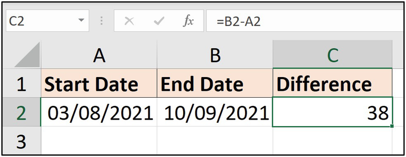
Calculating the difference between two dates
Days begin at midnight, so when calculating the date difference in this example, the day of 10/09/2021 (10th September 2021) is not included.

Date difference using the DAYS function
If you enter the start and end dates in the incorrect order (start date first), you will receive a negative value as the result.
Time in Excel
So, a date in Excel is referred to as a serial number and represents the value of 1. Time is part of a day, so it is represented as a decimal value.
For example, the time 06:00 is 25% of a day, or the value 0.25 in Excel, while the time 14:00 is 0.58 (rounded to two decimal places).
Now, I do not recommend telling your colleagues in the office that the time is 0.58. You may find yourself excluded from the tea round (is that just a British thing?).
These values would be formatted as time so that they are understood. However, it is very important that we understand how time is stored in Excel when using formulas.

Time and date and time shown in a general format
The method for entering the time can depend on your regional settings. In the UK, the colon “:” is used to separate hours, minutes, and seconds, for example, 08:30 or 09:35:12.
Other delimiters such as using a period or dot “ . ” to separate the hours, minutes, and seconds would not be accepted in the UK regional settings. However, they may be allowed in other regions.
Calculate the Difference in Two Times
As with dates, the difference in two times can be calculated by simply subtracting the start time from the end time.

Calculating the difference in two times
The TODAY and NOW Functions
Availability: All versions
The TODAY function in Excel returns the current date, while the NOW function returns the current date and time. The results of these formulas will update every time the worksheet calculates.
These functions are useful if you need to display the current date or date-time in a cell or perform calculations that require the current date or current date and time.
The functions will return the date and time information from the system clock of your computer. Figure 6-7 shows the TODAY and NOW functions returning values to a cell for display.
When using Excel for the Web , the date and time information is taken from the regional settings of where the workbook is located. Ensure your regional settings in OneDrive, the SharePoint site, or wherever the workbook may be stored are correct when using these functions.
The current date can be entered quickly in Excel with the Ctrl + ; keyboard shortcut. This is a faster alternative to typing the date and does not update like the TODAY function does.

TODAY and NOW functions displaying values in a cell
The TODAY function is useful for calculations that require the current date, for example, calculating the number of days until a deadline or due date. The results would need to update with time.

Calculating the number of days until a due date
The result may be returned in a date format. Strange, but true. To correct this, format the cell in the General format.
Convert Text to Date
The method for entering dates into Excel depends on your regional settings. I am based in the UK, so entering the date delimited by a slash “/” or a hyphen “-” is accepted, for example, 04/09/2021 or 04-09-2021. These are entered in the dd/mm/yyyy format. The name of a month can also be used, for example, 04 September 2021.
I would not be able to enter a date in the structure 04.09.2021 (although it can be formatted that way). It would be stored as text. However, in regions such as Germany, that structure would be accepted.
In the modern world, with data coming from a large variety of sources, dates can appear in a workbook in all shapes and sizes. When your Excel cannot translate a date as a date, you will need to convert it. We cannot work with the data until it is cleaned.
There are two main functions for this, DATEVALUE and DATE.
This is an Excel formulas book, so our focus is on formula solutions. They are often the perfect solution, as they are automated and can be combined with other functions. However, the Text to Columns and Power Query tools of Excel are also good options for converting date values.
The DATEVALUE Function
Availability: All versions
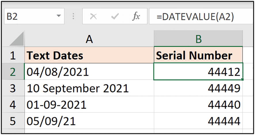
The purpose of the DATEVALUE function is to convert dates stored as text into dates. Or to be more specific, it converts them to their serial number, and then you would apply a date format to present them correctly.
DATEVALUE converting text dates to serial numbers
If the year is omitted from the text date, then the DATEVALUE function will apply the current year to the converted date. Figure 6-10 shows some examples of the DATEVALUE function doing this.

Converting text dates that are missing the year
Now, you can also convert the text dates by using them in a simple mathematical operation. The DATEVALUE function is unnecessary.

Converting text dates with a multiply operation
I am demonstrating this to show what is possible and not to downplay the use of the DATEVALUE function . The better approach is probably to use DATEVALUE, especially if others are using your spreadsheets. It is much more descriptive to others who are trying to understand what that formula does.
The VALUE Function
Availability: All versions
We saw the VALUE function in the previous chapter converting text to numeric values. It is worth mentioning again here as it can also convert text to date but has the additional ability to also convert time.

DATEVALUE function removing time from the converted text values
This is good if you want the time removed. Otherwise, let’s turn to the VALUE function .

VALUE function converts text values to date and time
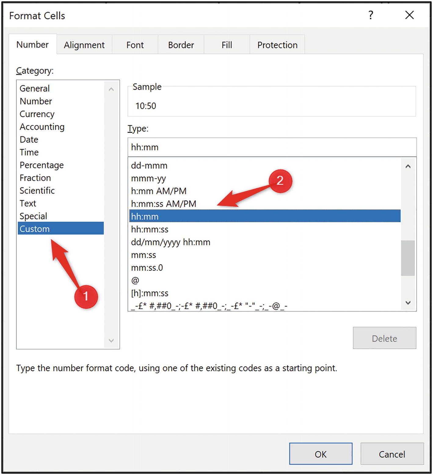
- 1.
Select the range to format.
- 2.
Open the Format Cells window by pressing Ctrl + 1 or by right-clicking the selected range and clicking Format Cells.
- 3.Click the Custom category and then scroll through the list of formats to find a date and time format to use (Figure 6-14).
 Figure 6-14
Formatting values as date and time

Converting text values to date and time easily
Although I demonstrate the example of multiplying the text values by one, other mathematical operations that do not change the number’s value also work. For example, you could use A2/1, A2+0, or A2-0.
The DATE Function
Availability: All versions
The DATE function returns the serial number that represents a date from a given year, month, and day.
Year: A number that represents the year
Month: A number that represents the month
Day: A number that represents the day
The DATEVALUE and VALUE functions are great when the text value is structured as a date. However, that is not always the case.
Another common structure is to receive date values in the structure yyyymmdd. This may be stored as a text value or a numeric value. It does not matter; the DATE function along with some text functions from the previous chapter can fix this.

DATE function creating a date from a number
Another scenario could be that the day, month, and year values are in different columns, when you import data from another source. This is a perfect scenario for the DATE function.

Creating a date from three separate values
And for a final example, the date can sometimes form part of a reference . I have a client I have worked with for years who store booking references in the format “21-08-02 AM.” This represents 2nd August 2021 with only two digits used to represent the year.
This formula concatenates the “20” to the two digits of the year to create the full year. Without this, it would likely convert 21 into 1921, instead of 2021.
The LEN function is used to help calculate the starting position of the day value.

Extract and create a date from a booking reference
So, the DATE function is a great function for converting values into a date. Another scenario for its use is to enter fixed dates into formulas. You cannot type dates directly into formulas due to Excel requiring the serial number.

Using DATE to enter a fixed date into a formula
Extract Date from a Date-Time Stamp
Often, when getting data from other sources such as a database, you will receive the date and time information.
There are several ways that you can extract the date from the date-time stamp if the time is not required.

#VALUE! error returned by the DATEVALUE function
To extract the date only from date-time values, we can use the INT or TRUNC functions.
The INT Function
Availability: All versions
The INT function rounds a number down to the nearest integer. This is perfect for the task at hand, as the time is the decimal part of the value, and INT will effectively nullify that.
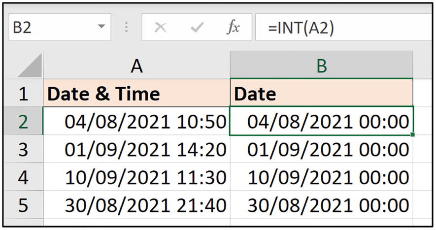
INT function extracting date from a date-time value
The TRUNC Function
Availability: All versions
The TRUNC function removes the decimal part of a number leaving only the integer. Once again, this is perfect for the task of removing the time from a date-time value.
Number: The number to truncate.
[Num digits]: A number to specify the precision of truncation. If omitted, 0 is used to remove the decimal part of the number.
The TRUNC function does not round values like INT and other functions. It simply chops the numbers off at the specified precision.
In this scenario of extracting a date from a date-time stamp, it makes no difference if you use INT or TRUNC, the result is the same.

TRUNC function extracting date from a date-time value
Although the official description of TRUNC is that it removes the decimal part of a number, this is only its default behavior.
For example, if you have a value of 728.91 in cell A2 and you use the formula =TRUNC(A2,-1), the value returned is 720 as it truncates one position to the left of the decimal. Or, if the formula was =TRUNC(A2,1), the value returned is 728.9 as it truncates to one position to the right of the decimal.
Extract Time from a Date-Time Stamp
To extract the time from a date-time stamp, we need to extract the decimal part of the value.

Extracting the time by subtracting the date element
Let’s look at how to extract the time element with the MOD function.
The MOD Function
Availability: All versions
Number: The number to divide
Divisor: The number that you want to divide the given number

Extracting the time with the MOD function
- 1.
Select the cells to format.
- 2.
Open the Format Cells window by right-clicking and click Format Cells or press Ctrl + 1.
- 3.
On the Number tab, click Custom and then select the time format from the list (Figure 6-25). The Custom category has been used instead of time to specify only hours and minutes.
The MOD function is a really cool function. I have personally utilized it over the years in several creative ways including to sum the values from every nth row.
Formatting the values to show time only in hours and minutes
The YEAR, MONTH, and DAY Functions
Availability: All versions
The YEAR, MONTH, and DAY functions are simple, yet very useful. They each extract their relevant part from a given date. Year will extract the year and so on.
In Figure 6-26, the YEAR, MONTH, and DAY functions have each been used to extract their element from the dates in column A.

YEAR, MONTH, and DAY functions
This example demonstrates how the functions work but is not a hugely practical example. We will see these functions being used later in this chapter to help calculate financial years and quarters. This will provide a greater insight to their use.
Let’s see another quick example before we leave them though. These functions can be used to extract part of a date for another function to use, for example, the IF function.
In this example, we want to apply a different rate dependent upon the time of the year. Dates from September onward require a different rate to other times of the year.

MONTH working with IF to test the month of a date
The NETWORKDAYS Function
Availability: All versions
The NETWORKDAYS function returns the number of whole workdays between two dates. Weekends (Saturday and Sunday) are excluded, and an argument is provided to specify additional non-working days that you want excluded.
This function is great for calculating the number of days worked on a task or project.
Start date: The start date to be used in the calculation.
End date: The end date to be used in the calculation.
[Holidays]: A range or array of dates that are considered non-working days. These could be national holidays or any other reason that the date is non-working. This is an optional argument.

NETWORKDAYS counts whole workdays
Figure 6-29 shows the number of days difference between the two dates in cells G2 and H2. The formula in cell I2 is a simple =H2-G2 date difference calculation.

NETWORKDAYS returning a different result
Calculate the Working Days Difference Between Two Dates
Let’s see a practical example of the NETWORKDAYS function. In this example, we need to calculate the number of days worked on the tasks of a project.
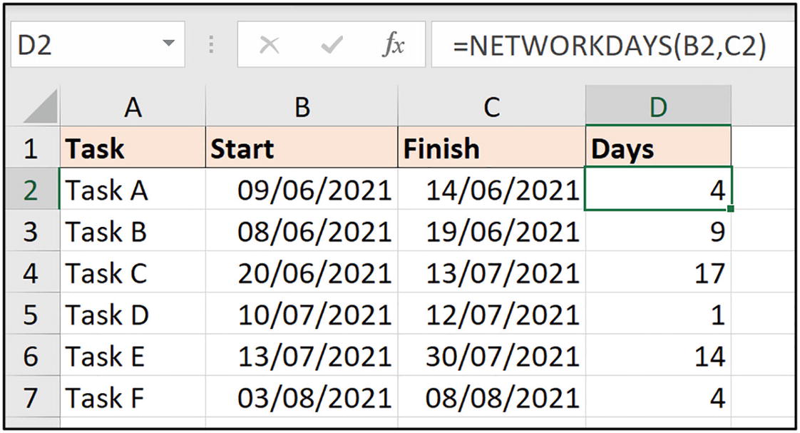
Calculating working days difference with NETWORKDAYS
Let’s specify additional non-working days for the formula to exclude. In Figure 6-31, the additional non-working dates have been entered into range L2:L6 and have been named [rngHolidays].

NETWORKDAYS with additional non-working days
The NETWORKDAYS.INTL Function
The NETWORKDAYS.INTL function performs the same role as NETWORKDAYS but with an additional argument to specify custom weekend parameters.

The weekend options in the NETWORKDAYS.INTL function
Let’s use the NETWORKDAYS.INTL function on the same range of dates and apply the Sunday only option for the weekend. This is known as option 11, as shown in Figure 6-32.

NETWORKDAYS.INTL with the Sunday only weekend option applied
Example 1: Customized NETWORKDAYS.INTL Function
The weekend argument of the NETWORKDAYS.INTL function can be customized to specify which days of the week are working and which are non-working. This provides much more flexibility in specifying non-working days than are offered by the weekend argument’s list of options.
The weekend argument can be entered as a text string of seven 1s and 0s. The first character represents a Monday and the other six for the remaining days of the week. A 1 is entered to indicate a non-working day, and a 0 is entered for a working day.
With this customization of the NETWORKDAYS.INTL function, it is easy to specify that you may only work on a project on Mondays and Tuesdays ("0011111") or that you may work Saturday only ("1111101") on a specific task.
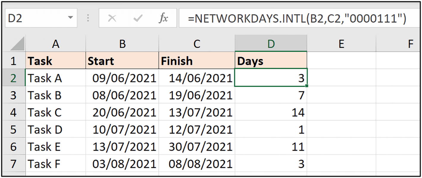
Specifying a working week of Monday-Thursday
Example 2: Conditional Holiday Ranges
Creating customized weekend parameters and specifying holiday ranges is great for accurate working days difference calculation. However, you may require different parameters or holiday ranges dependent upon a location or an individual.

Different non-working days by location

Conditional holiday range with NETWORKDAYS

Conditional weekend parameters with NETWORKDAYS.INTL
The first example utilizes defined holiday ranges, and the second example works with entered strings to specify the working and non-working days.

Table of non-working days by location

FILTER function returning the non-working dates for NETWORKDAYS
The FILTER function is covered in detail in Chapter 13. It is only available in Excel for Microsoft 365, Excel 2021, and Excel for the Web.
Example 3: Number of Fridays Between Two Dates
A unique use of the customized weekend parameter in NETWORKDAYS.INTL, shown in example 1, is to count the number of instances of a specific weekday between two dates. In this example, we will count the number of Fridays, but it could be any weekday or weekdays.

Formula to count the number of Fridays between two dates
This can also be achieved using the weekend parameters provided with the NETWORKDAYS.INTL function. Option 16 is the Friday only option.

Using the Friday only weekend option with NETWORKDAYS.INTL
The provided weekend options are limited. The text string offers more flexibility if you need multiple days, for example, Mondays and Thursdays between two dates.
The YEARFRAC Function
Availability: All versions
The YEARFRAC function returns the number of years and its fraction from a given start and end date. This can be very useful when calculating ages, proportions for annual benefits such as entitled leave, or financial interest between two dates.
Start date: The start date for the calculation.
End date: The end date for the calculation.
- [Basis]: A number that represents the day count basis (Figure 6-42). If omitted, 0 is used to apply the US (NASD) 30/360 basis. This means that each month of the year has 30 days.
 Figure 6-42
Day count basis options in YEARFRAC
The YEARFRAC function is great for calculating the number of years between two dates. And a great example for this task is calculating the age of someone or something.
Excel does not have a worksheet function to calculate age. This is quite a surprising omission. However, YEARFRAC makes it easy.
The day count basis has been specified as 1; this is the actual day count basis. So, it uses the actual number of days in each month. This is the most common basis to use. The other options apply for specific business uses.

Calculating years of service with YEARFRAC
Equally, the fractional part of the result could have been used to calculate proportional interest.
The DATEDIF Function
Availability: All versions
The DATEDIF function calculates the difference between two dates in a specified unit such as years, months, or days.
The DATEDIF function is unique in that it is undocumented in Excel. When you type the DATEDIF function in Excel, no information is provided (Figure 6-44).

DATEDIF function with no arguments showing
Start date: The start date of the calculation.
End date: The end date of the calculation.
Unit: Letters that represent the unit difference that you want to calculate. The characters must be entered within double quotes.
“Y”: The difference in complete years
“M”: The difference in complete months
“D”: The difference in days
"MD": The difference in days, ignoring years and months
"YM": The difference in months, ignoring years and days
"YD": The difference in days, ignoring years
Figure 6-45 shows examples of DATEDIF performing the more common unit entries.
Excel does not have a function for months difference, so the calculation of months difference and months difference ignoring years is of special interest.

DATEDIF function examples
Microsoft does not recommend the use of the “MD” unit. This is because it can produce an inaccurate result when calculating the remaining days after the last completed month. It is also why an example is omitted from this book.
DATEDIF function results can be combined to calculate the date difference in a string such as the number of years and months.

Date difference in years and months
The WORKDAY Function
Availability: All versions
The WORKDAY function is used to return the date a given number of workdays in the future or before a specified date. This function is very useful for calculating due dates, such as estimated task completion dates or expected delivery dates.
Start date: The start date for the calculation.
Days: The number of working days before or after the start date. Enter a negative value for days before the start date and a positive number for days after the start date.
[Holidays]: An optional argument that specifies additional non-working dates to be excluded from the calculation. They can be provided as a range of dates on a worksheet or an array returned by another function such as FILTER or XLOOKUP.
Let’s see some examples of the WORKDAY function in action.
Calculate a Due Date from a Starting Date
In this example, we have a list of tasks and their duration in working days. Based on this duration, we will use the WORKDAY function to calculate the estimated due dates.

Calculating estimated due dates for a list of tasks
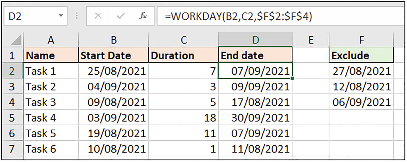
WORKDAY function including a holidays range
Remember, the WORKDAY function can also return a date a specified number of working days in the past. To do this, a negative value would be entered for the Days argument.
Although a less common scenario, the WORKDAY function could be used to calculate the start date from a given end date and number of working days.
The WORKDAY.INTL Function
Along with the WORKDAY function , there is also a WORKDAY.INTL function. This is a more flexible alternative to WORKDAY.
It can be used to customize the weekend parameter using a list of predefined options or to specify the working days of a week by entering a string of seven 1s and 0s.

Weekend options with WORKDAY.INTL

NETWORKDAYS.INTL function used to specify Sunday only
You can go beyond the standard options provided with WORKDAY.INTL by entering a text string of seven 1s and 0s. This provides us with a way of specifying whatever working week we require.
The first day in the string is a Monday. A 1 indicates a non-working day, and a 0 is a working day.

Entering a text string for the weekend argument of WORKDAY.INTL
The conditional holiday ranges and weekend options demonstrated in the section “The NETWORKDAYS Function” of this chapter can also be applied here to WORKDAY and WORKDAY.INTL.
Calculate First Working Day of a Month
It can be useful in some data analysis scenarios to calculate the next working day from specific date. In this example, we will return the first working day for the months of the year.

Dates presented as a month name

Calculating the first working day of a month
We will see how to calculate the last working day of a month, when we visit the EOMONTH function next.
EDATE and EOMONTH
Availability: All versions
The EDATE and EOMONTH functions return a date a specified number of months ahead or prior to an origin date. EDATE returns a date with the same day of the month as the origin date, and EOMONTH returns a date with the last day of the month.
Start date: The start date for the calculation.
Months: The number of months after or before the start date that you would like to offset the date. Enter a positive number to return a future date and a negative number to return a past date.
Calculate Contract End Dates
These functions are perfect for calculating future end dates such as contract finish dates.
Use EDATE if the end date is the same day of the month as the start date and EOMONTH if you need the last day of the month for the end date.

EDATE returning the date 12 months from the start date

EOMONTH returning the contract end date in 18 months’ time
Last Day of a Month
Instead of calculating a date a specified number of months into the future, maybe you want to return the date of the last day of a given month.
Calculating the last day of a given month
Number of Days in a Month
In a variation to the previous formula, maybe you do not want to return the date, but simply “how many days are in the month of a given date?”.

Returning the number of days in a given month
Last Working Day of a Month
By using the WORKDAY function and the EOMONTH function together, we can calculate the last working day of a month.

Calculating the last working day of a month
First Working Day of Next Month
Following the previous example, returning the first working day of the next month may appear straightforward. Once again, the WORKDAY and EOMONTH functions are combined.

Returning the first working day of the next month
The last two examples using WORKDAY were based on a working week of Monday-Friday. Remember, the working week can easily be customized to our requirements.
Returning Week Numbers
A common task in Excel is to return the week number for the year (calendar or fiscal), a project, or some other timeline.
Excel provides a couple of functions to calculate week numbers for years. For other scenarios, we can combine functions or be a little creative with our formulas.
The WEEKNUM Function
Availability: All versions
The WEEKNUM function returns the week number in the year. By default, it begins with the week that contains 1st January, but it can also return the week number according to the ISO 8601 standard.
Serial number: The date for the calculation.
[Return type]: A number that determines which day the week begins. By default, the week begins on a Sunday.
System 1: The week containing 1st January is the first week of the year. You can specify on which day the week begins.
- System 2: This system uses the methodology specified in ISO 8601. This is a universal standard for communicating dates internationally, removing any confusion. The week containing the first Thursday is week 1. Only return type 21 is used for this system.
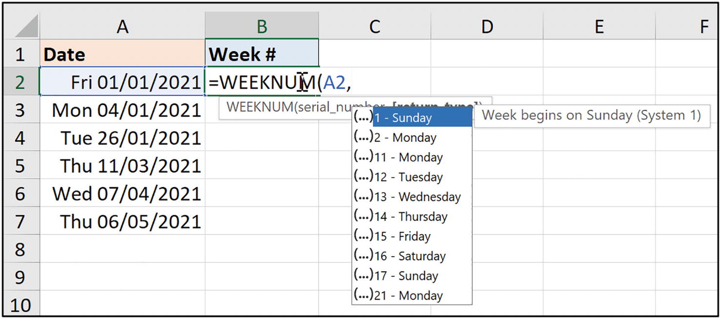 Figure 6-60
Return type options with WEEKNUM
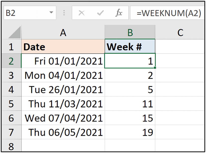
WEEKNUM using the default return type

WEEKNUM with the start of a week set as a Friday
The ISO 8601 standard defines the first week of a year as the week that contains the first Thursday. An ISO week begins on a Monday.
4th January 2021 is recognized as the first date of the first week of the year. This is because the first Thursday is 7th January 2021, and 4th January 2021 is the beginning of that week by ISO standards.

WEEKNUM using the ISO standard for week numbering
What Is ISOWEEKNUM?
The ISOWEEKNUM function returns the week number of the year as defined by the ISO standards for week numbering.
But didn’t we just accomplish this with the WEEKNUM function? Yes, we did. The ISOWEEKNUM function is redundant because WEEKNUM has option 21 that defines the use of the ISO standard.
However, I prefer the use of the ISOWEEKNUM function because its name is more descriptive than a function that defines option 21. Most people will not know what 21 means in the WEEKNUM function.

ISOWEEKNUM function returning week numbers
Return the Week Number for Any Given Date
Instead of returning the week number in the year, you may want to calculate the week number in a project, fiscal cycle, or maternity period. For this, we can write a simple little formula.

Returning the week number from any given date
The formula first finds the difference between the two dates in days. This result is then divided by 7 to return the number of weeks. Finally, 1 is added to the result. The TRUNC function has been used to remove the decimal part of the value.
So, for the date of 17th June 2021, the difference between this and the start date is 9. When divided by 7, the result is 1.28. 1 is then added to get 2.28. And TRUNC strips of the decimals.
Week Number in a Month
Another scenario could be to return the week number in a month instead of years. The WEEKNUM, or ISOWEEKNUM, function can be used within a formula to calculate the week number within a month.
The following formula uses two WEEKNUM functions (Figure 6-66). Using the date in column L, the first returns the week number in the year, and the second returns the year’s week number for the first day of that month.
The WEEKNUM function is using return type 2. This defines Monday as the first day of the week.
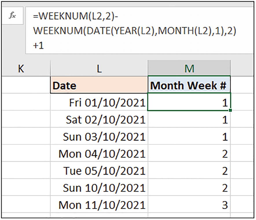
Returning the week number within a month
The WEEKDAY Function
Availability: All versions
The WEEKDAY function returns the day of the week of a given date. The day of the week is returned as an index number.
Serial number: The date of which to return the weekday.
[Return type]: A number that determines which day the week begins. By default, the week begins on a Sunday. So, Sunday = 1 and Saturday = 7.
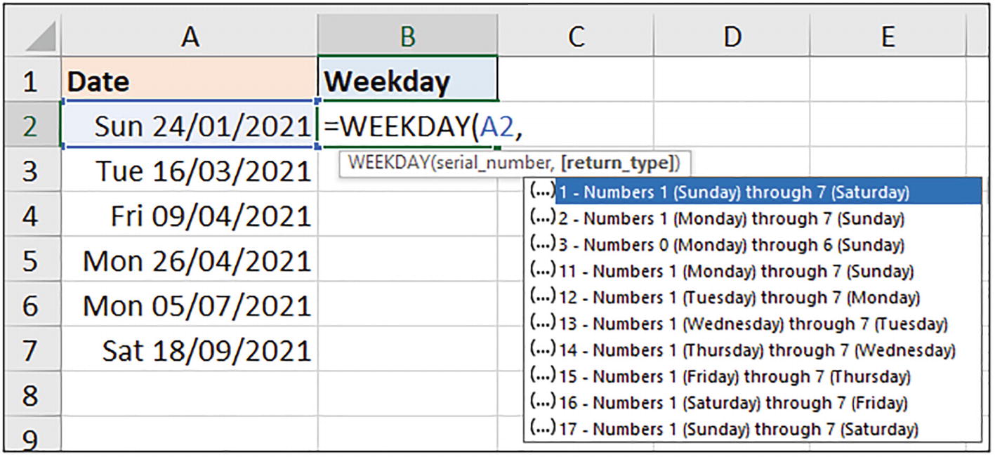
Return type options available for the WEEKDAY function
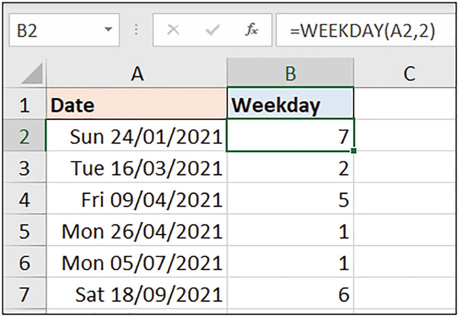
WEEKDAY function returning the day of week as a number
The dates in column A of Figure 6-68 have been formatted to show the day of week name so that we may see the accuracy of the formula easily. It is not necessary for the formula.
Rate of Pay Determined by Day of Week
Let’s now see a practical example of using the WEEKDAY function. In this example, we would like to apply a rate of pay that is dependent on the day of week when the hours were worked.
In this example, the staff will receive an increase in pay when they work on a Saturday or a Sunday. By setting the WEEKDAY function to return type 2, Monday = 1 and Sunday = 7, we can easily identify a Saturday or Sunday as their index number would be greater than 5.

Applying a different rate of pay dependent on the day of week worked
The WEEKDAY function is not required for tasks such as displaying the day of week name or sorting by day of week. The display of the weekday name in a cell can be achieved with some simple number formatting, and sorting by day of week in Excel is typically achieved using Custom Lists.
Calculating Financial Years and Quarters
For many countries, the financial year (also known as the fiscal year or business year) does not run from January-December, but from alternative start and end dates.
Let’s explore how we can calculate time periods such as financial years and quarters for some of the different financial years in operation in countries across the globe.
Fiscal Years
We will calculate the financial years for three different countries (India, Australia, and the UK) to get an understanding for the techniques involved. We will display the financial year as FY YYYY-YYYY, for example, FY 2021-2022.
Let’s dive into the formulas used for each calculation. The results for all three formulas are shown in Figure 6-70.
Indian Financial Year
The Indian financial year starts on 1st April and ends on 31st March. The following formula uses an IF function to test if the month of the date is later than March.
Australian Financial Year
The Australian financial year runs from 1st July to 30th June of the following year.
UK Financial Year
The financial year of the UK starts on 6th April and ends on 5th April. So, testing the month number of the date is not enough.
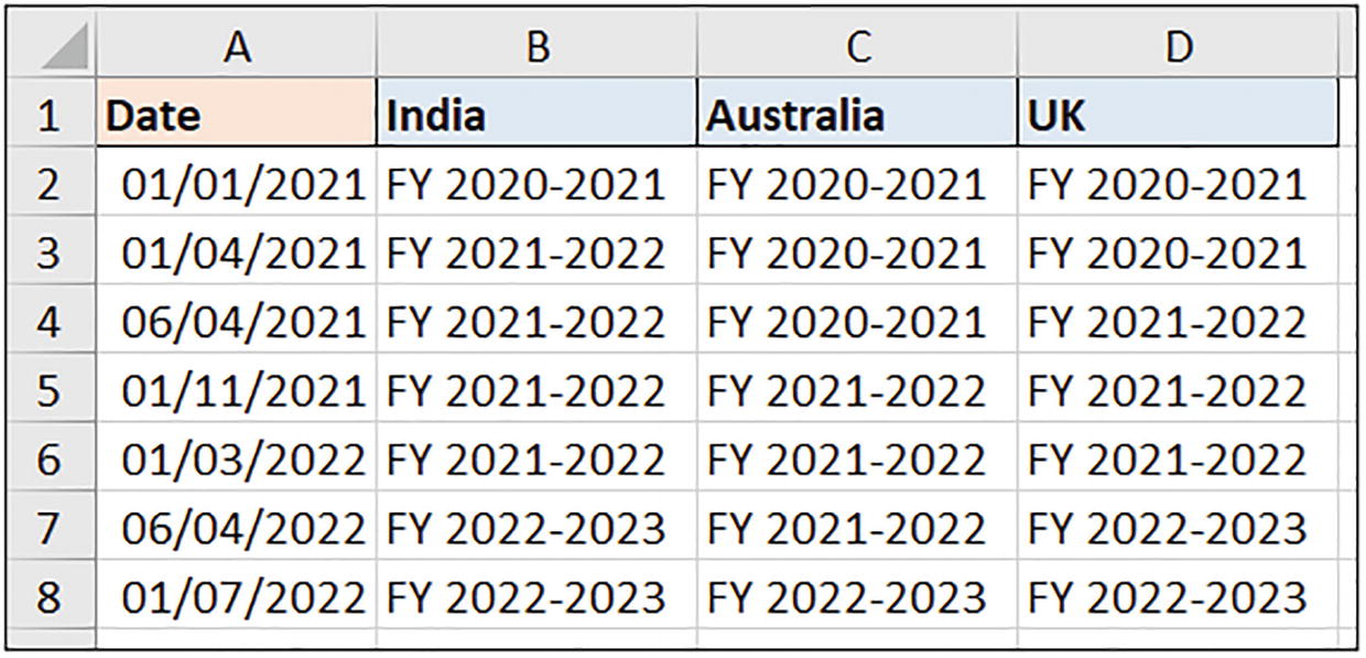
Financial year formulas for India, Australia, and the UK
Fiscal Quarters
The simplest way to calculate quarters for different company financial years is to use the CHOOSE function in Excel. So, we will start with an example using the CHOOSE function and then demonstrate an alternative method.
CHOOSE returns a value from a list of values based on an index number. This makes it perfect for quarter calculation. We can extract the month number from a date and use that as the index value to return the required quarter from a list.
The CHOOSE function is explained in detail in Chapter 11.
Let’s look at two different fiscal quarter formulas using CHOOSE. The results of both formulas are shown in Figure 6-71.

Fiscal quarter calculations with CHOOSE

Fiscal quarter calculations with CEILING and EDATE
The EDATE function is used to offset the date a specified number of months. The number of months to offset is dependent upon the first month of the fiscal year.
The number of months to offset is one less than the first month number of the fiscal year. If the year starts in April (4), then EDATE returns the date three months prior. And if the year starts in October (10), then EDATE returns the date nine months prior.
The MONTH function extracts the month number from the date returned by EDATE. The purpose of the CEILING function is to round a number up to a given multiple. In these formulas, CEILING rounds the month number up to the multiple of 3. And this result is divided by 3 to return the fiscal quarter.
Let’s see an example in action. We have the date of 1st July 2021 in cell F4. When returning the fiscal quarter for a year beginning in April, the EDATE function returns the date three months prior, so 1st April 2021 is returned. MONTH returns number 4 and CEILING rounds this up to a multiple of 3, which is 6. Then 6 divided by 3 is 2. The result is Q2.
For the same date but the fiscal year beginning in the month of October, EDATE returns the date nine months prior to 1st July 2021. The result is 1st October 2020. MONTH extracts the number 10, and CEILING rounds this value up to 12 (multiple of 3). 12 divided by 3 is 4, so the result is Q4.

The CEILING function is used for the rounding task in these formulas. This function is compatible with all Excel versions. In a formula example shortly, the CEILING.MATH function (an updated version of CEILING) will be used.
Working with Time
At the beginning of this chapter, we defined how time is stored in Excel and how it is structured. We also performed some simple calculations to find the difference between two times.
Let’s now dive into further important techniques to know when working with time in Excel.
Convert Text to Time
When receiving data from different sources, data does not always come in the format that we require.
To perform calculations and analysis on time data, it is imperative that Excel recognizes it as time. There are two main functions in Excel to convert text values into correct time values – TIMEVALUE and TIME.
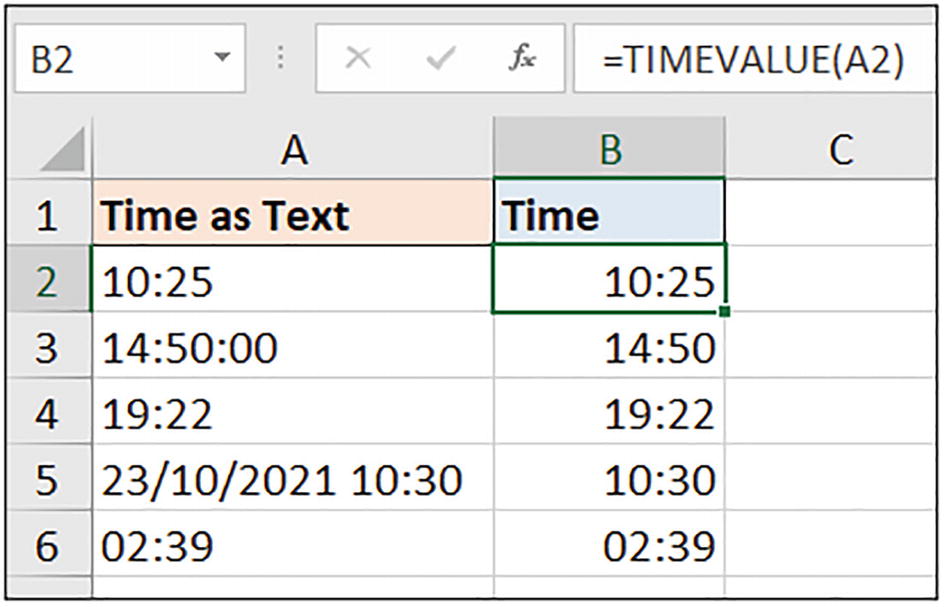
The TIMEVALUE Function
Availability: All versions
The TIMEVALUE function returns the time that is represented by text. It is quite simply the time alternative to the DATEVALUE function discussed earlier.

TIMEVALUE function converting text to time

Time formatting options all include seconds

Formatting time to show hours and minutes only
TIMEVALUE results correctly formatted
The TIMEVALUE function can only convert time that is stored as text. If the value you ask it to convert is not text, the #VALUE! error is returned.
Times stored as text can also be converted to time by using the VALUE function or by using a simple mathematical calculation that does not change the cell value.
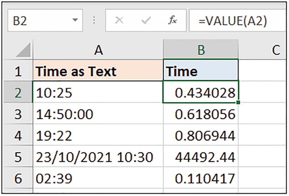
VALUE function converting text values into time

Simple mathematical operation to convert text to time
The TIME Function
Availability: All versions
The TIME function returns the decimal value that represents a time from a given hour, minute, and second.
This function is ideal when you need to convert to time from its different parts. For example, the hour, minute, and second may be in different columns on a sheet or extracted by different text functions from a value.
If the cell that the TIME result is returned to is formatted as General, a time format is automatically applied. This format can be changed or applied in advance.
In the first example of the TIME function (Figure 6-79), the hours and minutes in the text values are separated by a period, or dot. My UK regional settings do not recognize these values as a legitimate time format; therefore, the TIMEVALUE function would not convert them. It produces the #VALUE! error instead.
The following formula uses the LEFT and RIGHT functions to extract the hour and minute from the value. These are passed to the TIME function to create the time value.

TIME function converting time stored as text
Although this section is about converting text to time, it is worthwhile seeing an example of time being stored as an incorrect numeric value.
In this example, a spreadsheet has been generated from an export, and the time values contain the period or dot separator again. However, this time, my regional settings have forced Excel to assume that the dot is the decimal separator.

TIME fixing incorrect numeric values
Text functions such as FIND and LEN are covered in detail in Chapter 5.
For the minute argument of TIME, an IF function is nested to test if the number of characters representing the minute is only one character, for example, 14.5. If it is, then a “0” is appended to the minute string. So, 14.5 would become 14.50; otherwise, instead of being converted to 14:50, it would become 14:05.
In this formula, the calculation to return the minute is used three times. In Chapter 15, we will cover the LET function. This function helps us to create more efficient and meaningful formulas, and this formula is a good use case for LET (available in Excel for Microsoft 365, Excel 2021, and Excel for the Web versions only).

Convert decimal number to time including the LET function
The TEXTBEFORE and TEXTAFTER functions, available in modern Excel and covered in Chapter 5, could also have been used to simplify the formula. However, the original formula is compatible for all Excel versions.
For the final TIME function example, we see another common representation of time, which is to display the hours and minutes without any separator (Figure 6-82). The values are stored by text in Excel and need converting.

Converting text values with TIME
Rounding Time
There may be situations when you need to round time values. Time can be rounded to any multiple of significance – hour, 30 minutes, 15 minutes, etc.
There are three key functions for rounding time: MROUND, CEILING.MATH, and FLOOR.MATH. Let’s quickly cover how each of these functions operates before we see them in practice rounding time.
MROUND, CEILING.MATH, and FLOOR.MATH
The MROUND, CEILING.MATH, and FLOOR.MATH functions all round values to a multiple of significance. The function you use depends on how you wish to round.
The CEILING.MATH function always rounds up to the nearest multiple. It also requires the number to round and the multiple of significance.
The CEILING.MATH and FLOOR.MATH functions were first released with Excel 2013 as improved functions to their predecessors – CEILING and FLOOR. If you use a version before Excel 2013, the CEILING and FLOOR functions work perfectly well too.
Round Time to the Nearest Hour
In Figure 6-83, the three functions have each been used to round time to the nearest hour.

Rounding time to the nearest hour
Round Time to the Nearest 15 Minutes
Figure 6-84 shows further examples of these three functions rounding time values. In these examples, time is rounded to the nearest 15 minutes.

Rounding time to the nearest 15 minutes
Time Difference Past Midnight
Calculating the difference between two times in Excel is actually very simple. It is the formatting of the results that can be frustrating.
When the time difference is over 24 hours, the formatting can be even more tricky. In Figure 6-85, the results of the formula =G2-F2 are shown in column H.

Time difference in General format
- 1.
Select the range H2:H6 and press Ctrl + 1 to open the Format Cells window.
- 2.
On the Number tab, click the Custom category.
- 3.
Type the following into the Type field (Figure 6-86):
d "days," h "hours" - 4.Click OK.
 Figure 6-86
Applying custom formatting to show days and hours
The duration values are now more legible (Figure 6-87). Custom formatting is an incredibly powerful tool in Excel, and it can be used to format values exactly how we want.

Time difference formatted in days and hours
You may notice in the duration results that three of the five results do not exceed 24 hours.
So, let’s set a condition in our formatting rule to format the results that are over 24 hours in the format “x days, x hours” and results less than 24 hours in the format “x hours.”
Select the range H2:H6 and open Format Cells to edit the existing custom number formatting code.

Setting a condition in your custom number formatting
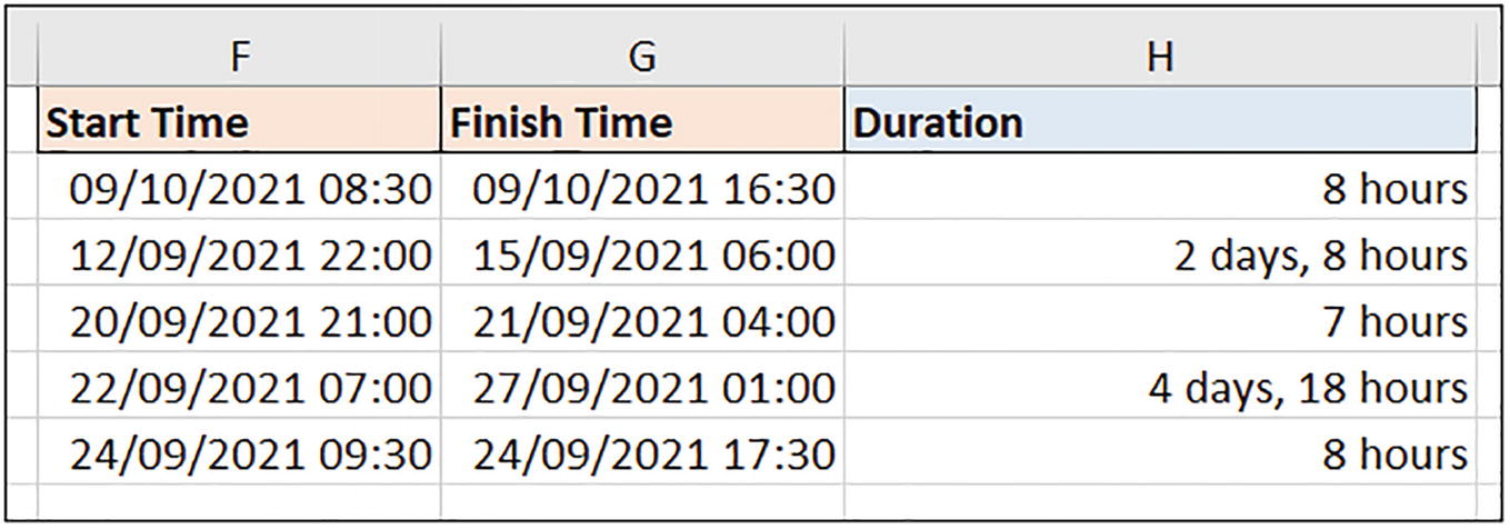
Formatting to display hours only when less than 24 hours
Sum Hours over 24 Hours
It is very common to display a result as total hours, even if it spans multiple days. After all, what is a day? Is a day 24 hours? Or is it 8 or 9 hours such as a typical business day? It is open to interpretation.

Sum of total hours with the same days and hours formatting
There is a special formatting trick to display the total hours that exceed 24 hours in Excel. That trick is to enclose the “h” within square brackets.
An “h” without square brackets will only display the remaining hours past a multiple of 24 hours.
- 1.
Select range H2:H6 and cell H8 and press Ctrl + 1 to open the Format Cells window.
- 2.
On the Number tab, click the Custom category.
- 3.
Type the following into the Type field:
[h] "hours" - 4.
Click OK.

Formatting time to show hours over 24
Handling Negative Time
Excel cannot display negative time, so this can create a problem if you need them. Fortunately, there are always workarounds for problems such as this.
In Figure 6-92, we have the London Marathon finish times for the men’s category for the last six years. In column D, a formula is calculating the time difference compared to the previous year.
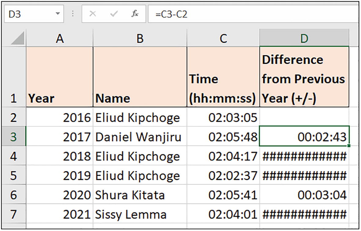
Negative times cannot be displayed in Excel
Let’s look at two methods to display negative time in Excel.
The first method is to switch the Excel workbook from its 1900 date system to the 1904 date system.
This will fix the negative dates; however, be careful, because changing the date system will change any existing dates in the workbook. The dates will be adjusted by four years.
- 1.
Click File ➤ Options ➤ Advanced.
- 2.
In the When calculating this workbook section, check the Use 1904 date system box (Figure 6-93).
- 3.Click OK.
 Figure 6-93
Switching to the 1904 date system
The negative times are now displayed correctly (Figure 6-94). If you notice this causes a problem with dates on your spreadsheet, you can easily come back to the Excel options and turn off the 1904 date system.
The results are also still numeric values. This is useful if you need to perform further calculations on them. The next approach will convert them to text to display them correctly.

Negative times displayed correctly in Excel
The second method uses the TEXT function (covered in Chapter 5) to display the negative time values as text, but in a time format.
We will also take this opportunity to hide the hours from the results, as a marathon finish time will never be more than 60 minutes improved on a previous year.

Formula to display negative time values
Date and Time Functions with Other Excel Features
Let’s now see a few practical examples of date and time functions being used with other Excel features.
Highlight Approaching Due Dates
A common requirement in Excel is to track due dates. These could be payments that are due, contracts expiring, or deadlines of project tasks.
With the array of date functions available in Excel, we can set almost any conditions we may need. Let’s see a few examples.

- 1.
Select range B2:B7.
- 2.
Click Home ➤ Conditional Formatting ➤ Highlight Cells Rules ➤ Less Than.
- 3.
Enter the following formula into the Format cells that are LESS THAN: box (Figure 6-97):
=WORKDAY(TODAY(),10) Figure 6-97
Rule to format dates due within the next ten working days
- 4.
Specify the cell formatting from the list and click OK.

Two dates identified as being due soon
You will see different dates and possibly different results to what are shown in the images. The dates are calculated by a formula to remain current, and the results of WORKDAY are based on the TODAY function and so are determined by the date that you read and practice this.
- 1.
Select range B2:B7.
- 2.
Click Home ➤ Conditional Formatting ➤ Highlight Cells Rules ➤ Between.
- 3.
Enter the following formulas into the two Format cells that are BETWEEN: boxes (Figure 6-99):
=WORKDAY(TODAY(),10)and=WORKDAY(TODAY(),20) Figure 6-99
Rule for dates due between the next 10 and 20 working days
Unfortunately, this window is not resizable, so the full formulas could not be shown in the image.
When editing formulas in Excel windows, be careful of the active cell mode. Using the cursor arrows on the keyboard while in “Point” mode causes chaos in your formula. The different cell modes of Excel were explained in Chapter 1.
- 4.
Specify the cell formatting from the list and click OK.

Two formatting rules highlighting due dates
Highlight Dates Due Within the Next Month
Let’s add one more quick Conditional Formatting example, as an opportunity to recap on another function we saw in this chapter. That function is EDATE.
In this example, we want to highlight the dates due within the next month. This is often done by testing if a date is within the next 30 days. And this method is often sufficient, because we just want to bring the date to our attention and the result does not need to be that precise.
- 1.
Select range B2:B7.
- 2.
Click Home ➤ Conditional Formatting ➤ Highlight Cells Rules ➤ Less Than.
- 3.
Enter the following formula into the Format cells that are LESS THAN: box (Figure 6-101):
=EDATE(TODAY(),1) Figure 6-101
Rule to format due dates within the next month
- 4.
Specify the cell formatting from the list and click OK.

All except one date occur within the next month
Data Validation Rules – Prevent Weekend Entries
As an example of date functions being used in Data Validation rules, let’s prevent the entry of weekend dates in a cell.
In this example, we will assume the weekend to be Saturday and Sunday; however, this can easily be customized for any day(s) of the week.
- 1.
Select the range that you want to apply the Data Validation rule to. Range E2:E6 has been used for this example.
- 2.
Click Data ➤ Data Validation.
- 3.
Click the Settings tab of the window.
- 4.
Click the Allow drop-down and select Custom.
- 5.
Enter the following formula into the box provided (Figure 6-103):

Validation rule to prevent entry of weekend dates
- 6.
Click the Error Alert tab and enter a meaningful Title and Error message to appear if a user enters a date that is a Saturday or Sunday (Figure 6-104).
- 7.Click OK.
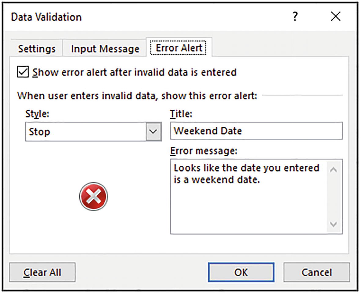 Figure 6-104
Customized error alert for users

Invalid date entry being rejected by the validation rule
Summary
In this chapter, we learned the most useful date and time functions in Excel supported with numerous examples of their application in the “real world.”
The chapter began with a detailed explanation of how dates and times are stored in Excel and how to effectively enter, convert, and extract dates and times. This topic is often misunderstood by Excel users, yet it is so critical to the performance of your calculations.
We then embarked on a tour of many different functions including WORKDAY, NETWORKDAYS.INTL, EDATE, and TIME. We performed many formulas including to find working days, return fiscal months and quarters, and return week numbers in a year or from a specific start date.
This chapter was very comprehensive and should act as a guide to refer to whenever you need a particular date or time calculation.
In the next chapter, we will learn the VLOOKUP function in Excel. This notorious function is extremely useful and is one of the most commonly used functions in Excel. Because of this, an entire chapter is dedicated to it.
You will learn how to use the VLOOKUP function including some insider tricks to make it more powerful, flexible, and dynamic. You will also understand common mistakes that users make and should be avoided.