
VLOOKUP is one of the most used functions in Excel. Almost anyone who has used Excel for a certain number of years would have heard of VLOOKUP and has likely written one or two.
This function is often considered a benchmark in a user’s Excel development – that moment when they step into the intermediate level of Excel formula skills. I will never forget the days when I was first learning VLOOKUP – a wild mixture of confusion, fun, and excitement.
In recent years, with the development of the new array engine in Excel (Chapter 10) and with new functions such as XLOOKUP and FILTER, the position of VLOOKUP as the number 1 lookup function of Excel is beginning to get a little shaky.
Make no mistake though. This function is incredibly useful, very popular (used in millions of spreadsheets worldwide), and therefore important for an Excel formula jedi to master.
VLOOKUP is available in all versions of Excel, so is reliable when sharing spreadsheets to staff across different offices or to users external to your organization.
In this chapter, we will begin with the basics of VLOOKUP and learn how to write the two different types of lookups (exact match and range lookup). We will learn some neat VLOOKUP tricks and understand common reasons to why things go wrong.
As the chapter progresses, we will see more advanced uses of VLOOKUP including using multiple lookup criteria and returning a specific instance of a value.
vlookup.xlsx
Introduction to VLOOKUP
Availability: All versions
The name VLOOKUP stands for vertical lookup. It looks for a value, within a table, and returns a value from the same row but from a different column in the table.
The VLOOKUP function always looks for a value in the first column of the table in which it is told to search.
There are many reasons VLOOKUP is used. The most common use is to look up values in another table to combine them into one main table. This table would then be used for the analysis such as a PivotTable.
Other reasons include to compare two lists for differences, automate data entry on a spreadsheet, and fetch values from a lookup table for use in calculations, for example, a lookup table of different tax rates by city.
Lookup value: The value you are looking for.
Table array: The table or range that you are looking and returning from.
Col index num: The number of the column containing the value you want to return. This is the column number within the table array, not the worksheet.
[Range lookup]: A logical value (TRUE or FALSE) to specify whether you are looking in ranges of values or not. This is an optional argument.
TRUE is used to request a range lookup (also known as an approximate match). This is the default option. FALSE is used to specify an exact match.
VLOOKUP for an Exact Match
The most common form of VLOOKUP is to perform an exact match. This means that you are looking for a unique value such as a product code, booking reference, or an employee ID.
In this first example, we have a table named [tblTiers] that contains the prices for different membership tiers (Figure 7-1).

Lookup table with tier prices
Although the second argument of VLOOKUP is named table array and this example uses a table, it should be noted that it does not need to be a table. It could be a range such as $B$2:$C$7, a named range, or an array returned by another function.
VLOOKUP looks vertically down the first column of a given table. In this example, that is the [Tier] column of the [tblTiers] table.
FALSE is used to specify an exact match in the final argument.
The tiers in [tblTiers] are in ascending order by the [Price] column and not by [Tier]. This demonstrates that when performing an exact match, the table array does not need to be ordered by its first column.
The column index number is 2. [Price] is the second column in the [tblTiers] table.

VLOOKUP to return the price for each membership
For the range lookup argument, a 0 can be entered to request an exact match instead of False, and a 1 can be entered to specify a range lookup instead of True.
VLOOKUP for a Range Lookup
The second type of lookup that you can perform with VLOOKUP is a range lookup. With this type of lookup, you are looking within ranges of values. For example, these could be date or time ranges or other values such as exam scores, amounts spent, or some other performance value.
This type of lookup, although not as commonplace as an exact match lookup, can be very useful. Let’s see two examples.
In the first example, we have the lookup table shown in Figure 7-3. The first column contains a range of quantity values. We have a table of orders and want to look up the quantity ordered and return the earned discount.
When performing a range lookup (also known as an approximate match), it is essential that the first column of the lookup table is in ascending order.

Range of quantities and discounts to look up
The lookup range is not formatted as a table, so has been referenced in the formula as 'Range Lookup Data'!$A$2:$B$7.
TRUE has been entered for the range lookup argument to specify an approximate match.
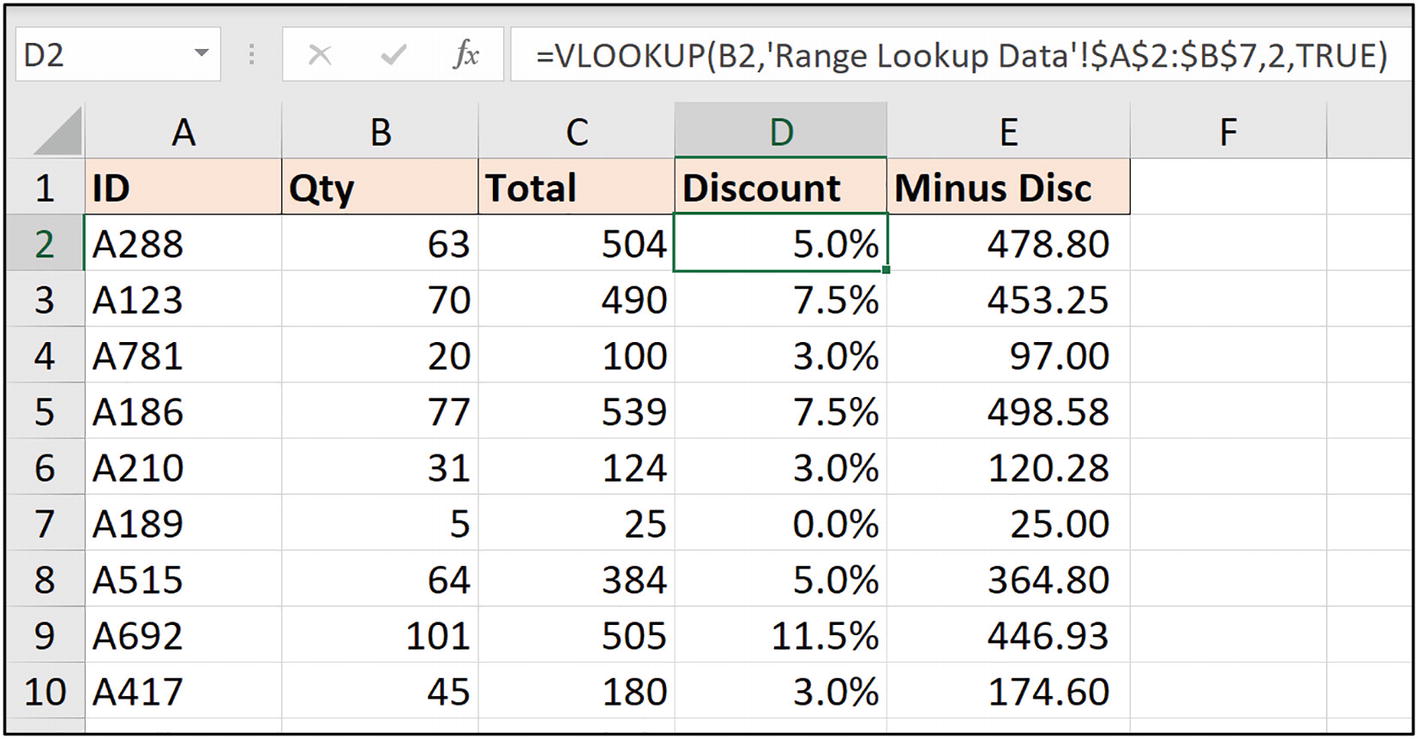
VLOOKUP returning the appropriate discount of each quantity ordered
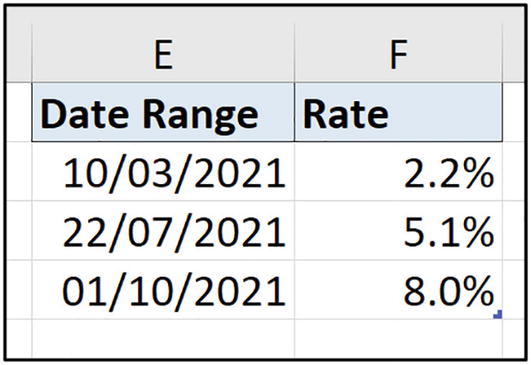
Lookup table with date ranges and tax rates

Returning the tax rate dependent upon the date of transaction
Column Index Number Tricks
In the examples demonstrated so far, the lookup tables have been small, and the column index number has always been 2. When looking up data in larger tables, counting to find the correct column index number can be frustrating.
There are a few tricks that we can deploy to save having to count to find the required column index number. These tricks also work in making our VLOOKUP formulas more durable, as when typing the number directly into the formula, it can easily be broken by someone inserting or deleting a column.
Another mistake can be that a user did not count hidden columns when finding the column index number.
Trick 1: The COLUMN Function
Availability: All versions
The COLUMN function returns the column number of a given reference. This reference can be a cell, table column, or a named range. It returns the column number of the sheet, for example, column D is column number 4.
This function is ideal for the task of preventing having to find the column number in the lookup table ourselves. We can just reference the column of the lookup table that we want, and COLUMN returns its index number.

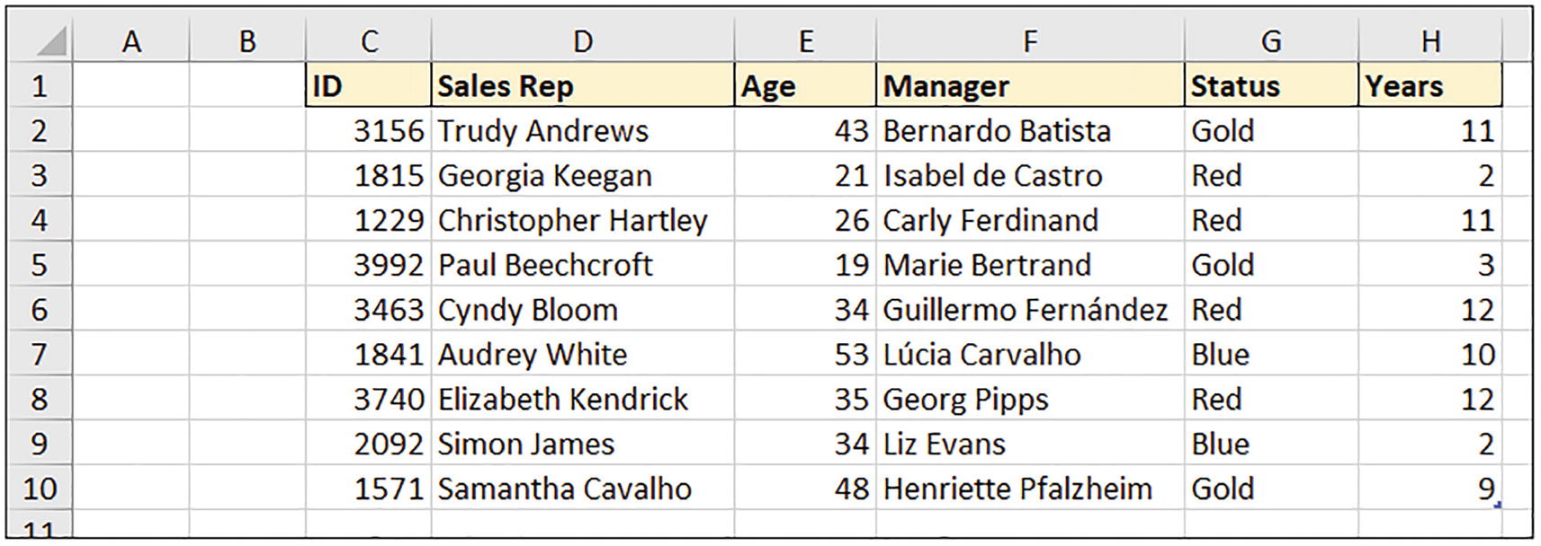
Sales representative data
The COLUMN function is provided with the [Status] column of the table. This makes it very simple to provide a column number to VLOOKUP, as referencing columns in a table is fast and easy. This technique was covered in Chapter 4.
Remember, the column number returned is the column number of the worksheet, not the table.

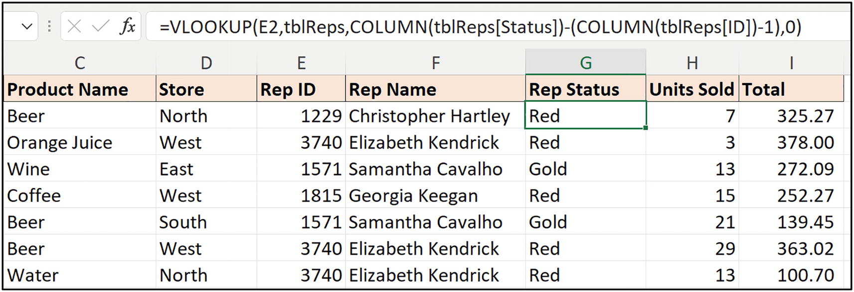
COLUMN function used to prevent entering the column number
Lookup table beginning from column C
For the COLUMN function to work, we will need to subtract two from its result to account for columns A and B not being used by the table.

VLOOKUP function with COLUMN to fetch the column number
If someone were to insert another column, or remove a column, before the start of the table, our formula would fail. The subtraction of 2 would no longer be relevant.
For a more robust version of this formula, we want to dynamically return the column number of the column directly before the table, 2 in the previous example. To do this, the COLUMN function will be used to return the sheet’s column number of the first column of the table. One will be subtracted from this to return the column number that precedes the start of the table.
More robust version of VLOOKUP with the COLUMN function
Trick 2: The COLUMNS Function
Availability: All versions
The COLUMNS function returns the number of columns in a given reference or array. This could be a reference to a range of cells, a table, a named range, or an array formula.
This function is very useful when the column number you require is at the end or a specific number of columns from the end of a reference or array.
In Figure 7-12, we have a table named [tblMonthly] that contains monthly performance values for staff. We require a VLOOKUP to return the last month’s performance. This will always be the final column in the table (currently May-21).
The COLUMNS function will be perfect for this task, as every month the table will expand with another column when a new month is added. The COLUMNS function will always return the number of columns in the table, that is, the final column number.
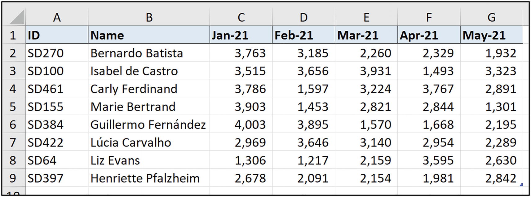
Table with staff monthly performance

COLUMNS function used to return the final column’s data
There are also ROW and ROWS functions in Excel to perform the equivalent tasks but for rows instead of columns. We will see ROWS later in this book.
Trick 3: Using an Index Row
Another technique that you may come across is the creation of an index row. This is a row where the column index numbers of the table are entered and then referenced in the VLOOKUP.
Figure 7-14 shows an index row set up above a lookup table. Notice that the lookup table range begins in column B, but the column is indexed as column 1, ready for VLOOKUP. This lookup range is on a sheet named [Index Row Data].

Lookup table with an index row

VLOOKUP referring to a cell value to return the column index number
Referring to a cell value in this manner is another trick to avoid counting the columns of your larger lookup tables.
It is not as durable as using the COLUMN function can be, but it is very simple to set up and utilize.
Another technique is to use the MATCH function to find and return the required column number. We will see this technique in Chapter 11, when we explore more lookup functions in Excel.
Reasons Why VLOOKUP Is Not Working
There are a few reasons why your VLOOKUP is not working. Let’s explore some of the common reasons along with their solutions.
Lookup Column Must Be the First Column
VLOOKUP looks for a value down the first column of a given range or array. If the column you need to look in is not the first (or leftmost) column of the table array, VLOOKUP will not find a match.

The lookup column needs to be the first column
This can be fixed by reordering the columns of the lookup table so that the ID column is first or by using a different formula to VLOOKUP, such as XLOOKUP or the INDEX-MATCH function combination.
Another fix in this example is that you do not need to select all the columns of a table or range, only the ones that you need.

VLOOKUP now works with an adjusted table array
Data Type of the Values Must Match
This issue causes problems even for regular users of VLOOKUP. The data type of the lookup value and the value it finds must match, not just its value.
This issue commonly occurs when the table array is an export from an external source, and the numeric values are stored as text. However, the lookup value is a number.

VLOOKUP not working due to problem with the data type
The fix is to convert either the lookup value to text or the values in the lookup column to numbers. Which side you convert depends on what the value should be – text or number.
Figure 7-19 shows the values in G6:G9 converted to numbers and the VLOOKUP now working.
The Text to Columns command in Excel provides a quick way to convert text to numbers. You need only to select the values, click Data ➤ Text to Columns and then click Finish to close the window for a quick conversion.

ID values are converted to numbers and the VLOOKUP works
This issue can be confusing and difficult to detect. Figure 7-20 shows the numeric values in range G6:G9 selected. They are left aligned and have a text format applied, so do not appear as numbers.
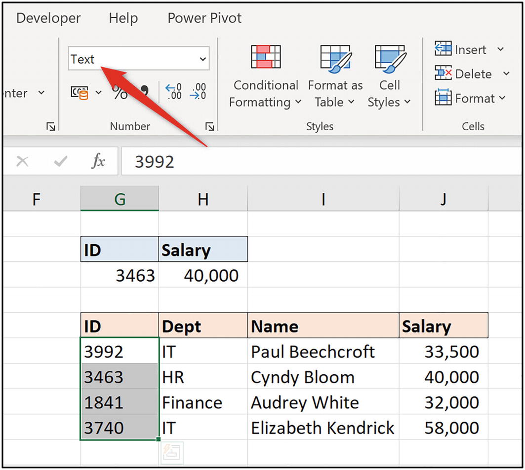
Numbers appearing as text can be confusing
When diagnosing issues such as this and it is unclear what data type a value is, the information functions such as ISNUMBER and ISTEXT are very helpful. They check if a value is a number or is text and will return TRUE if it is a match.

ISNUMBER function confirming the data type of values
Exact Match Has Not Been Specified
This is a common mistake for users that are new to using VLOOKUP. So, keep an eye out for this on spreadsheets set up by others that include VLOOKUP.
The final argument of VLOOKUP is range lookup. This argument is confusing when you are getting started with this function, it is optional, and TRUE is the default. These three factors seem to lead to the argument being missed or ignored.
If you require an exact match but do not specify one, you run the risk of having the wrong results and errors returned.
In Figure 7-22, the final argument is omitted when an exact match is required. You can see the incorrect result for ID 3992 in cell C6. There is also an error in cell C3 for ID 1841.

VLOOKUP returning incorrect results and errors

Exact match is specified and the VLOOKUP works
Ranges Must Be in Ascending Order
As we already know, the ranges need to be in ascending order when performing range lookups (approximate match lookups). If a lookup table has been ordered differently for any reason, this will present a problem for VLOOKUP.

Ranges not in order breaking VLOOKUP
To fix this issue, the first column of the lookup table needs to be sorted into ascending order.

VLOOKUP working now that the ranges are in ascending order
Handling Fake Errors with VLOOKUP
Now, not all errors that VLOOKUP returns are real errors. VLOOKUP is very eager to return #N/A if it cannot complete its job. And sometimes there are logical and valid reasons why it cannot complete its job.
In these circumstances, an alternative action is desired over the error returned by VLOOKUP.
In this example, we have a simple claim form for mileage expenses in Excel. When a user specifies the site that they traveled to, we want a VLOOKUP to return the distance in miles of that site.
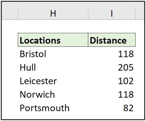
Lookup range with locations and their distance
Figure 7-27 shows the mileage claim form. There are some empty rows where there are no expenses to claim.
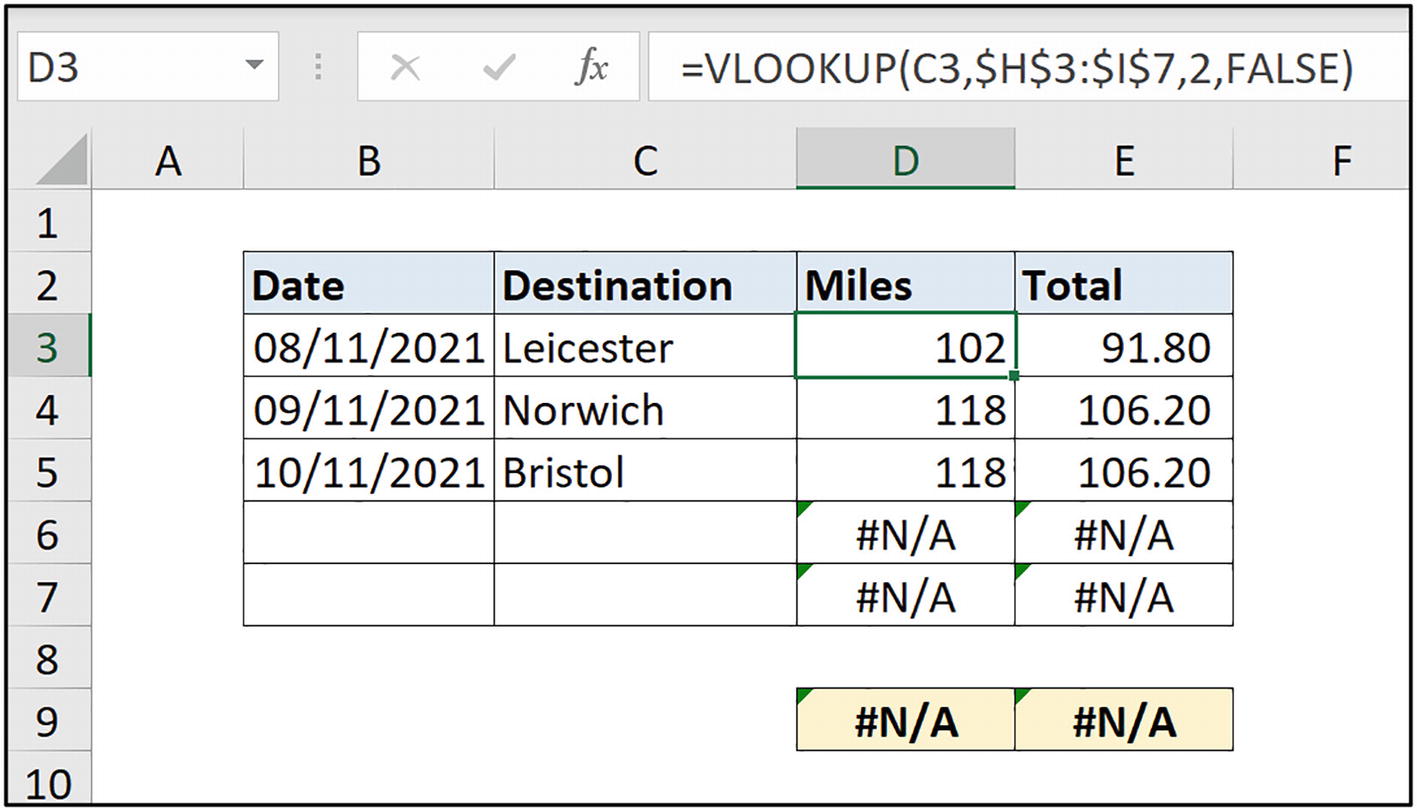
VLOOKUP returning errors for the empty destination cells
There are two main functions for this task – IFERROR and IFNA. These functions use the same syntax and were covered in detail in Chapter 2, so we will dive straight in and use these now.
The IFERROR function will return an alternate action if any error is returned by VLOOKUP; IFNA focuses on the #N/A error only.
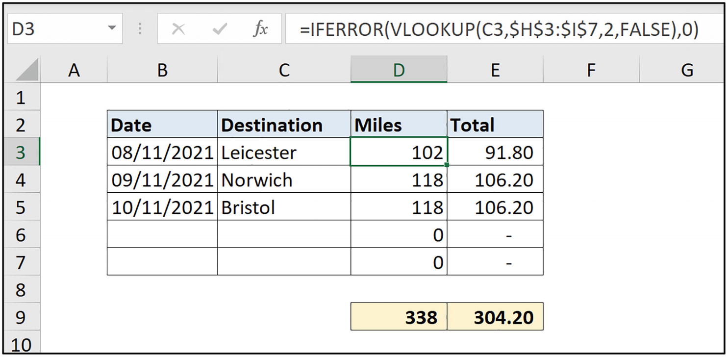
IFERROR function added to replace errors with 0
Although entering the value 0 is used in this example, we could have displayed any value or run an alternate formula.
The HLOOKUP Function
Availability: All versions
VLOOKUP has a lesser-known sibling – HLOOKUP. As you may have guessed, this stands for horizontal lookup.
Due to its less common usage compared to VLOOKUP, we will see only one example of HLOOKUP. However, every example demonstrated with VLOOKUP in this chapter can be performed with HLOOKUP, if required.
Figure 7-29 shows a lookup table/range with weekly performance values relating to some individuals. The headers are in the first column of the range (column B) with each field’s data stored in rows.

HLOOKUP returning the value from the fifth row of the lookup range
Get VLOOKUP to Look to the Left
One of the limitations of VLOOKUP is that it can only return a value from a column to the right of the one containing the lookup value (the first column).
Now this is not often a problem, as the first column of a table is typically a unique identifier. However, there is a trick to get VLOOKUP to look to its left.
Take the example shown in Figure 7-30. We need a VLOOKUP to return the grade for the score earned by each person.

VLOOKUP returning errors as the score is not the leftmost column
This trick requires the use of the CHOOSE function in Excel. The CHOOSE function will change the order of the columns for VLOOKUP to work from.
The CHOOSE function returns a value, or performs an action, from a list of given values and actions. The value or action it chooses from the list is based on an index number.
The CHOOSE function is used in the table array argument of VLOOKUP. It is given the array of constants {1,2} for its index number. It is then told to return range $G$3:$G$6 first and $F$3:$F$6 second, therefore reversing the column order.
This is an array formula, so press Ctrl + Shift + Enter to run it if you are not using Excel for Microsoft 365, Excel for the Web, or Excel 2021.
The CHOOSE function is covered in more detail in Chapter 11, when we explore more lookup functions.

CHOOSE function included to change the column order
This technique is fun and good to be aware of. However, for a more flexible lookup formula, the INDEX and MATCH combination or XLOOKUP functions in Excel are encouraged.
Partial Match Lookup
A partial match is when only part of the lookup value text needs to match. Sometimes, you may be looking to perform a partial match instead of an exact text match.
For example, Figure 7-32 shows a table named [tblTargets]. It contains the performance targets for different offices that are in different cities. The [City] column contains the country name in addition to the city.

Table of offices and their respective targets
The VLOOKUP function allows the use of wildcard characters directly in the function. This makes it easy to create partial matches with VLOOKUP.
* (Asterisk): Represents any number of characters. For example, New* would match with Newport, Newcastle, New York, and New Zealand.
? (Question mark): Represents a single character. For example, L????n would match with both London and Lisbon.
~ (Tilde): Used to treat a wildcard character as a text character. For example, *don would match any text that ends in the characters don, but ~*don will look for an exact match of *don, treating the asterisk as its character and not a wildcard.
The asterisk is joined after the city name in cell C3. Perfect for this scenario. We do not know how many characters will follow the city name, but we know there will be some.

VLOOKUP with a wildcard character for a partial match
Case-Sensitive VLOOKUP
Excel formulas rarely consider the case of characters when matching values. There are exceptions to this, for example, the FIND function is case-sensitive.
Figure 7-34 shows a VLOOKUP formula returning incorrect results for the lookup values written in lowercase – a and b.

VLOOKUP returning incorrect results due to case discrepancy
To create a case-sensitive VLOOKUP, the CHOOSE and EXACT functions will be used together. This is an advanced example that creates a two-dimensional array for VLOOKUP to use.
We saw an example of EXACT being used to match case in Chapter 2 of this book. Back then, we were working with the IF function. Let’s quickly remind ourselves on the EXACT function.
The EXACT function compares two text strings to see if they are exactly the same, including their case. It returns True if they are the same; otherwise, False is returned.
We saw the CHOOSE function two examples ago, when we made VLOOKUP look to its left.

Case-sensitive VLOOKUP formula
So, how does this work?
The VLOOKUP function has been given the lookup value of TRUE, so it now looks for TRUE down the first column of the two-dimensional array it has been given and returns the value from the second column.
Multiple Column VLOOKUP
It may be that you have two or more columns that need to be used in a lookup. VLOOKUP was not made with this scenario in mind, and it is much easier to perform with a function such as XLOOKUP or with a Merge Query in Power Query.
However, of course, it can be done. In Figure 7-36, we have a table (columns G:I) named [tblLastMonth] that contains a [Regional Code] column and a [Client ID] column along with last month’s [Total] value.

Sample data with two columns to match with our lookup
We will do this by first creating a new column in [tblLastMonth] with the combined [Regional Code] and [Client ID]. This column will be the one used for the lookup, so it needs to be the first column of the table.
- 1.
Right-click any cell in the [Regional Code] column of the table.
- 2.
Point to Insert and click Table Columns to the Left (Figure 7-37).
- 3.
Type the header “Reference” for the new column.
Note You can also insert a table column by clicking Home ➤ Insert ➤ Insert Table Columns to the Left.

Insert a table column to the left of the first column

Reference column from combined regional code and client ID

Multicolumn VLOOKUP formula
This technique can easily be extended to work for more than two columns, if required.
Taking this a step further, you can create a multicolumn VLOOKUP using a single formula. So, we can achieve this without inserting a new table column and creating the merged [Regional Code] and [Client ID] column.
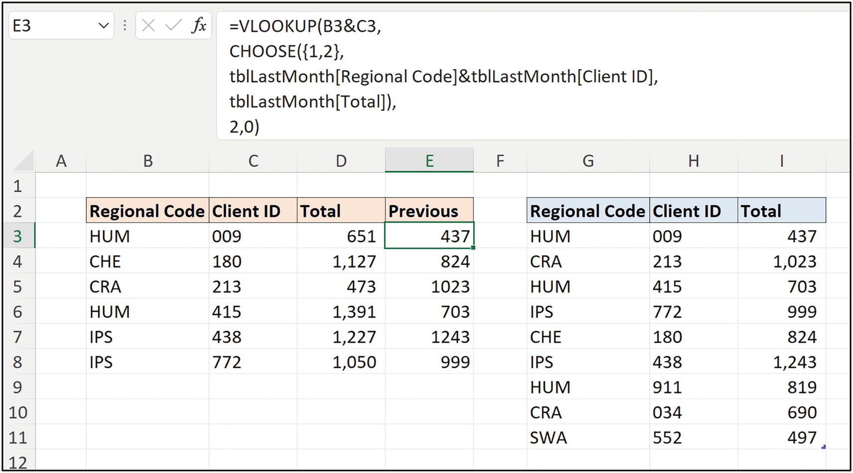
Multiple column VLOOKUP with a single formula
We saw the CHOOSE function recently when getting VLOOKUP to look to its left. This brilliant function is covered in more detail in Chapter 11.
Return the Nth Match
The VLOOKUP function always returns a value for the first occurrence of the lookup value that it matches, searching from top to bottom.
Now, if you want to return multiple results, this is not something that VLOOKUP can do. You want to use the FILTER function, covered in Chapter 13.
We can however use VLOOKUP to return a specific instance of the lookup value, such as the second, third, fourth, or nth instance.
In Figure 7-41, we have a lookup range that contains multiple instances of participant names and their scores in a contest. Each participant has three attempts, so they occur three times.

Multiple occurrences of participant scores
Like the previous example, our first task is to create a lookup column in the first column position of the lookup table that we can use to uniquely identify each instance.
The COUNTIFS function (covered in Chapter 8) is used to count the occurrences of each name.
The interesting part of this formula is the criteria range given to COUNTIFS. It has an absolute cell reference at the start of the range and a relative cell at the end of the range. This ensures that the criteria range expands as the formula is filled down the cells of column E.
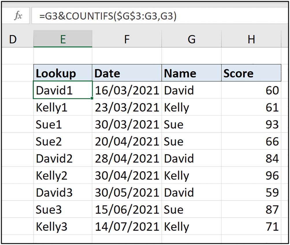
Lookup column with name and instance number combined

VLOOKUP returning the first, second, and third instances of a value
It is possible to achieve the same result using a VLOOKUP formula without the helper column identifying each unique instance. It is a more advanced formula.
So, how does this formula work?

Returning the Nth match with a single VLOOKUP formula
The SMALL function then returns the Nth smallest number in this array. This number is specified by the values in range B5:B7. For the formula in cell C5, the SMALL function returns 4 as that is the first smallest number.
The CHOOSE function is used in the table array argument of VLOOKUP (Again! What a useful function!). It creates an array consisting of two columns.
In column 1, the ROW function returns a list of the sheet row numbers for range $F$3:$F$11. The result is {3;4;5;6;7;8;9;10;11}. Column 2 is simply the values from range $G$3:$G$11.
The VLOOKUP function searches for the row number returned by the SMALL and IF combo, in the column of row number provided by ROW, and returns the score value from column 2 of the array created by CHOOSE. Awesome!
VLOOKUP with Other Excel Features
As always, we will conclude the chapter with some examples of how VLOOKUP can be used with other Excel features. Let’s see two examples, one with Conditional Formatting and another with a chart.
Conditional Formatting and VLOOKUP
For a Conditional Formatting example, we want to format the values that exceeded a target score. The target score resides in a different table to the one with the formatted values, so we will use VLOOKUP to retrieve it for testing.
Figure 7-45 shows a list of staff, their locale, and their performance value. A second table lists the different targets by locale.

Performance values and a separate target by locale table
- 1.
Select range D3:D9.
- 2.
Click Home ➤ Conditional Formatting ➤ New Rule ➤ Use a formula to determine which cells to format.
- 3.
Enter the following formula into the Format values where this formula is true: box (Figure 7-46):
It is often easier to type a formula into a cell first and then copy and paste it into the Conditional Formatting rule. The formula box is quite small and offers little help, and you need to be careful to be in the correct cell mode when moving through the formula.
- 4.
Click Format and specify the formatting you want to use.
- 5.
Click OK to apply and close each window.

VLOOKUP in a Conditional Formatting rule
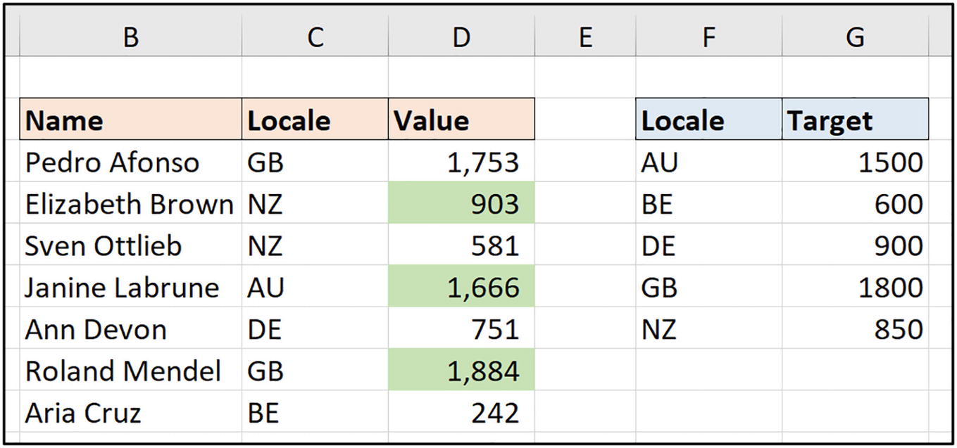
Formatting rule to format only values that are >= the target value
Dynamic Chart Range
In this chart example, we will create a dynamic chart range that changes on the selection of a value from a drop-down list.
In Figure 7-48, there is a table named [tblWeekly] with six weeks’ performance data by different staff members. Below the table are headers in preparation for our range that will feed the chart, and in cell J3 is a drop-down list of the different staff members’ names.

Table of data with a chart range below and a list in cell J3
Typically, the table of data, chart range, and chart with drop-down list would all be on different worksheets – a data sheet, calculation sheet, and a report/presentation sheet. It is displayed all-in-one here only to show the mechanics of the technique easier.
The COLUMN function is used to return the column index number so that we do not need to enter it ourselves in six different VLOOKUP formulas, when we fill the formula.

VLOOKUP formula for a dynamic chart range
- 1.
Select range B11:H12.
- 2.
Click Insert ➤ Insert Line or Area Chart ➤ Line.
- 3.
Make the necessary improvements to the chart to make it look awesome.

Dynamic chart based on the value from the drop-down list above it
Creating the chart is explained very briefly here as working with charts is not the purpose of this book. It is the formulas and the creation of the dynamic chart range that is our focus.
Summary
In this chapter, we learned the VLOOKUP function in Excel along with some tricks to creating a more robust and effective VLOOKUP formula and an understanding of common mistakes that users make. We then progressed to some advanced examples that included multi-criteria and case-sensitive lookups.
In the next chapter, we will look at formulas that perform aggregations such as sum, count, and average dependent on conditions that are met. There is a group of functions in Excel built for these purposes. This group includes SUMIFS, COUNTIFS, and AVERAGEIFS.
There are similar functions, also covered in the next chapter, just outside the scope of this group that includes MEDIAN, TRIMMEAN, and MODE.MULT.
Using functions such as these to aggregate values based on conditions is very popular in Excel. We have lots to cover, so let’s get started.