
There is a group of functions in Excel that perform conditional aggregations. The two most well-known functions of this group are the SUMIFS and COUNTIFS functions. However, this also includes the AVERAGEIFS, MAXIFS, and MINIFS functions.
These functions are quick to learn, as they look very similar to each other. So, once you know one, you kind of know them all. They are an incredibly useful group of functions, especially COUNTIFS.
In this chapter, we will begin with the SUMIFS function. We will understand its syntax and how to write the different logical tests and see multiple examples of its use. This will also build an understanding for the other functions in the group as we progress through the chapter.
We will then explore the brilliant COUNTIFS function and the other functions in the group. The chapter also covers formulas to achieve similar tasks that are just outside the scope of this group of functions.
The SUMIFS Function
Availability: All versions
sumifs.xlsx
The SUMIFS function sums the values in a column, for the rows that meet one or more criteria. For example, sum the sales values for sales of a specific product, or sum the attendance values for a specific training course in a specific region.
This is a wonderful and well-rounded function. It is simple to use and works very well with table data and with arrays (we will see array examples in Chapter 10).
Sum range: The values to be summed. This can be a range, table column, or an array.
Criteria range1: The range or array of values to be tested using criteria1. If the criterion is met, the corresponding value from the sum range is summed.
Criteria1: The criterion to be evaluated in criteria range1. This can be entered as a string, a number, or an expression. The following are all valid ways to enter the criterion: “London”, B4, “<”&B4.
[Criteria range2], [Criteria2], ...: Additional criteria ranges and associated criterion when testing more than one condition.
The size of the criteria ranges and the sum range must be the same.

tblSales data to be used for the SUMIFS examples
SUMIF or SUMIFS

SUMIF and SUMIFS functions in intellisense list
The SUMIF function was essentially made redundant when Microsoft released the SUMIFS function with Excel 2007. The SUMIF function can only test one condition, while the SUMIFS can do one or more conditions.
Now, the SUMIF function is heavily used to this day and, therefore, is important to understand, despite its redundant nature.
Notice the key difference is that the SUMIF function begins with the criteria range argument, while SUMIFS begins with the sum range argument due to its handling of multiple conditions.
From this point, the book moves on only with the SUMIFS function, but be mindful that SUMIF can achieve the same examples, but for a single condition only.
There are also COUNTIF and AVERAGEIF functions to accompany the COUNTIFS and AVERAGEIFS functions we see later. However, there is no singular version for MAXIFS and MINIFS.
Using Text Criteria
For our first example, we will use the SUMIFS function to test a single condition. We will sum the values in the [Total] column for the sales from the East store only.
The text value “East” has been entered directly into the Criteria argument of the SUMIFS function. Table references are used for the [Total] and [Store] columns.
SUMIFS works wonderfully with table data. These references make the formula easier to read and ensure that the sum range and criteria range are of equal size.
The SUMIFS function is not case-sensitive. Entering “East” or “east” for the criteria is both accepted.

SUMIFS function with criteria entered directly
However, you probably agree that this is less efficient. It is harder to understand, is not dynamic, and is more prone to user error. The many advantages of using tables were outlined in detail in Chapter 4.
By entering the criteria directly into the Criteria argument, it is a constant. This could be an advantage of its use. But, if we want the user of the spreadsheet to be able to easily change the store being summed, then the formula can reference a cell value, instead of having the criteria “hardcoded” into it.

SUMIFS function using a cell value for the criteria
Working with Multiple Criteria
Continuing with the previous example, we will use the SUMIFS function with two conditions. We will sum the values in the [Total] column for a specific product and store. The product and store will both be specified by cell values.

SUMIFS function with two conditions
In this example, AND logic is used between the two conditions, and this is the desired response. The SUMIFS function cannot handle OR logic natively. We will see a little trick for OR logic with SUMIFS shortly.
Using Numeric Criteria
Testing numeric criteria with SUMIFS is quite different to how numbers are tested in functions such as IF.
Remember that with SUMIFS, the criteria must be entered as text, a number, or an expression. So, you can enter a number into the criteria, but if you want to test if the number is “>=”, “<”, or some other logical test, then this must be entered as text or written as an expression.

SUMIFS function with a numeric condition entered directly
If you want to use a cell value for the number criteria, then the logical characters can be combined with the cell value using an ampersand (&).

SUMIFS function with text and cell values combined for criteria
Sum Values Between Two Dates
The SUMIFS function is perfect for the task of summing values with date conditions.
In this example, we will sum values between two dates. However, the scenario could be to sum values with a single date condition, for instance, the values since a specified date or until a specified date.
Remember, dates in Excel are numbers. So, the technique used is a repetition of the previous example when we tested numeric criteria.

SUMIFS to sum values between two dates

Adding separate SUMIFS functions to create an OR logic result
Additional criteria could be added to test for a specific product or store. The SUMIFS function can handle up to 127 conditions.
OR Logic with SUMIFS
The SUMIFS function performs AND logic between its corresponding criteria ranges and criterion. SUMIFS does not support the use of OR logic in its truest form. So, many users would produce a separate SUMIFS for each condition that forms part of the OR expression and add the result of each SUMIFS together.
This works fine. However, there is a trick to perform OR logic with multiple conditions. Let’s see some examples of how to do this.
Continuing to use the data in the [tblSales] table, we will sum only the values in the [Total] column that match multiple specified regions.
In this first example, the store regions are entered directly into the formula as an array of constants (Figure 8-10).

Array of constants in SUMIFS for OR logic with multiple conditions
This is great, but I am sure you are thinking – can we refer to cell values instead of typing the text directly into the array?
Well, yes you can. And to take it further, if we format the range of cells as a table, it will create a dynamic criteria range that we can easily add and remove criterion to and from.

Using a table as the source for OR logic values

SUMIFS criteria range expanded
In non-dynamic array–enabled versions of Excel, you need to press Ctrl + Shift + Enter for the formulas that reference a range for OR logic.
When using a range or an array of constants for OR logic, you can still take advantage of the up to 127 criteria offered by the SUMIFS function (and its friends).
The SUMPRODUCT and SUM (in Excel for Microsoft 365 and 2021 versions) functions offer great alternatives to SUMIFS when the logic gets more complex.

SUMIFS function with both AND and OR logic included
The examples so far have focused on text criteria only. And this is much more likely to be required. However, the same technique can be used with numeric criteria too.
Both date ranges are formatted as tables ([tblDates1] and [tblDates2]), so that they can be easily referenced and expanded or reduced, if required.

SUMIFS summing values between two date ranges
Using Wildcards with SUMIFS
The SUMIFS function and the others in its group allow the use of wildcard characters. These wildcard characters allow us to perform text matches in our criteria that are similar but not exact.
Asterisk (*): The asterisk is used in place of any sequence of characters. It is fantastic for performing partial text matches and is the more commonly used wildcard character. For example, the criterion “*America” can be used to match both “South America” and “North America.”
Question mark (?): The question mark is used in place of a single character. This is useful when the matching text needs to be a specific number of characters. For example, the criterion “SR???” will match any five-character text string that begins with “SR”. It would match “SR371,” but not “SR9271,” “SR4,” or “DF736.”
If you need to use an actual asterisk or question mark within the criteria, precede the asterisk or question mark with the tilde (~) character. The tilde forces the function to use the actual character and not treat it as a wildcard.
Let’s look at two examples of using the SUMIFS function with wildcard characters. These examples use the [tblOrders] table on the [Wildcard Characters] worksheet.
The asterisk has been entered as text (enclosed in double quotations) and concatenated to the value in cell B3.

SUMIFS function with the asterisk wildcard character

SUMIFS function with the question mark wildcard character
The Versatile COUNTIFS Function
Availability: All versions
countifs.xlsx
The COUNTIFS function counts the number of times its given criteria are met. It can handle up to 127 corresponding criteria ranges and criteria.
This makes the COUNTIFS function an exception in this group, as all the other functions require a column to aggregate – sum, average, maximum, and minimum.
The COUNTIFS function works in the same manner as the SUMIFS function before, except it counts instead of sums. All the examples demonstrated with SUMIFS, including testing numeric criteria, the use of wildcard characters, and handling OR logic, also apply to COUNTIFS.
These techniques also apply to the AVERAGEIFS, MAXIFS, and MINIFS functions. They all have the same fundamental way of working.
As the COUNTIFS function works in the same way as SUMIFS, we will not repeat the same examples. However, let’s look at a couple of simple COUNTIFS formulas to get a feel for this function.
The following two examples use the same [tblSales] table that was used for the majority of the SUMIFS examples before.

COUNTIFS function with a single condition

COUNTIFS with more than one condition
The COUNTIFS function is one of my favorite functions. It is very versatile and has been a savior many times over the years for me.
So, let’s see a few examples that are a little outside the traditional scope of how it is used.
You can expect to see more of the COUNTIFS function later in this book. It is an incredibly useful function, and there are future examples of it being used with functions such as FILTER, SUMPRODUCT, and MIN to achieve specific objectives.
Comparing Two Lists
The COUNTIFS function is fantastic for the task of comparing two lists. If you are trying to find the items that appear in one list but not another, or maybe you want to know the items that do appear in both, COUNTIFS is ideal for these tasks.

Two lists to compare and identify the missing values
We will use the COUNTIFS function to count the occurrences of the names in the first table in the second table. This will flag to us if the names are present in the second table or not.
The [Name] column of [tblSecond] is given as the criteria range, and the name in the current row (the @ symbol indicates this row of a table) is given as the criteria.

COUNTIFS function returning the number of times the names appear
Now, this is serving a purpose, but it would be nice to have a more meaningful output than a bunch of 1s and 0s. So, let’s wrap an IF function around our COUNTIFS to request a different response to be returned.

IF function added to return a more meaningful result
We will see the COUNTIFS function comparing lists again in Chapter 13 of this book. It will be used with the FILTER function to return only the matching or missing rows.
Generating Unique Rankings
There are functions in Excel that will rank values in a range in either an ascending or descending order. However, independently they do not create a unique ranking if any of the values are tied.
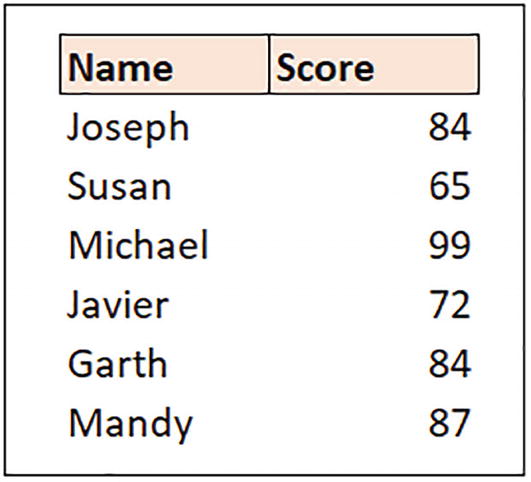
Table of scores to be ranked highest to lowest
Now, you might be thinking, why don’t you just sort the list by the score values? Well, sure we could do this.
However, we would like an automated process that ranks them as the scores are added or changed. Also, by using formulas we could create something more complex and rank by other conditions, if required.
To rank the score values, we will use a function named RANK.EQ, a function that ranks a number relative to the other numbers in a list.
Number: The number whose rank you want to return.
Ref: The range of numbers to rank the number within.
Order: The order to rank the numbers. Enter 0 or omit the argument to rank in descending order. Enter 1 to rank in ascending order.
The RANK.EQ function was released in Excel 2010 as the successor to the RANK function. The RANK function still exists for compatibility reasons. There is also a less common RANK.AVG function that is not covered in this book.

Ranking values in a range using RANK.EQ
We need to return a unique rank for each score. This is so that we can use a lookup formula to generate a table with the names and scores ordered by their rank.

Unique ranking calculated with COUNTIFS and RANK.EQ
Let’s break that down a little more.
Joseph’s score is the first occurrence of the score 84 in the range $C$3:$C3. So, COUNTIFS returns 1. A 1 is subtracted from this result and then added to the rank. This means that the rank does not change.
Garth’s score is the second occurrence of the score 84 in the range $C$3:$C7. So, COUNTIFS returns 2. A 1 is subtracted, leaving 1. And this 1 is added to the rank to become a rank of 4.
The COUNTIFS function has helped us create a unique ranking which the rank functions of Excel could not do alone. Amazing!
To complete this task, we will now order them by their rankings. And for this, we will use the VLOOKUP function that was covered in Chapter 7.
Remember, the VLOOKUP function looks down the first column of a range and returns from a column to its right. Currently, the unique rankings are in the last column. So, we need to change this before we start writing a VLOOKUP.
- 1.
Select range D2:D8 and cut the cells.
- 2.
Right-click cell B2 and click Insert Cut Cells from the context menu (Figure 8-25).

Insert cut cells to quickly move a range of cells
We can now create a rankings table and use the VLOOKUP function to return the names and scores in order by looking up their rank.
In Figure 8-26, rankings have been typed in column F and then VLOOKUP functions written into columns G and H to return the required information.

VLOOKUP function to return the scores in the order by rank
In later chapters, we will see functions such as INDEX-MATCH and XLOOKUP. These functions can perform the lookup without the need to have moved the column first. Until now, we have only covered VLOOKUP, so therefore took that approach.
It should also be noted that in Chapter 7, we did see a formula that used VLOOKUP with CHOOSE to overcome the built-in limitation of VLOOKUP only looking down the first column of its table array. That technique could have been applied instead of moving the column.
Creating Conditional Rankings
Let’s take the rankings example a step further, and instead of using the RANK.EQ function , we can do it all with COUNTIFS. Not only that, but let’s add another condition.
In Figure 8-27, we have a table named [tblRegionalScores] with names and scores that are divided into three different regions.

Table with scores from different regions
The COUNTIFS function tests the region and then returns how many scores are larger than the score in that row. 1 is then added to this result.
The 1 is added because if there are 0 scores larger than the current one, then that score is rank 1. If there is 1 score larger than the current one, then that score is rank 2, and so on.
So, the COUNTIFS function can create rankings on its own and can include any extra conditions that may be required.

Conditional ranking formula that creates rankings for each region
We can use the same technique as we did previously and add a COUNTIFS function to this result to generate a unique ranking.
This is similar to how we added COUNTIFS to the RANK.EQ function before. However, this time we do not need to subtract 1 like earlier, because we replaced the plus 1 from the first COUNTIFS.

Second COUNTIFS to make the ranking unique
From here, we could create separate ranking tables for each region or whatever our end goal may be.
But the focus of this chapter is COUNTIFS, so with this result, we will move on.
Creating a Frequency Distribution
For the final COUNTIFS example, let’s create a frequency distribution table. Excel has a function named FREQUENCY for this purpose, but it is limited when compared to COUNTIFS.

Table of scores and a bin range
We want to return a count of the scores in each bin. To do this, we will include the LEFT and RIGHT functions that were covered in Chapter 5 to extract the lowest and highest values in each bin range for testing.
The LEFT and RIGHT functions are used to extract the first two and last two characters from the ranges in column E for testing.

Frequency distribution created with COUNTIFS
This frequency distribution table could be the result, or it could be used as the source for a histogram for a graphical representation.
The AVERAGEIFS Function
Availability: All versions
averageifs.xlsx
The next function in our journey through the IFS family of functions is AVERAGEIFS. It returns the mean average for the values that meet the given criteria.
The AVERAGEIFS function requires the range of values to perform the average calculation on and the up to 127 criteria range and criteria pairs.

The tblSales table showing product sales
We want to return the average of the values in the [Total] column for a specified product and region.
The AVERAGEIFS function is like the SUMIFS function earlier in the chapter, so there is no need to go into much detail on how this works.
One of the many great things about this group of functions is how similar they are. Once you are familiar with one, you know them all.

AVERAGEIFS function to return the average sales value
In Figure 8-34, we have a table named [tblRegionalScores], and there are a couple of zero values in the [Score] column.
When performing an average calculation, these zero values are included by the function, and this may not be the behavior that we want. The result of an AVERAGE function is shown in cell E3.

Table of scores that include zero values
This is a cool use of the AVERAGEIFS function. Of course, with its ability to handle multiple criteria, we could return the average for a specified region in addition to excluding the zero values.
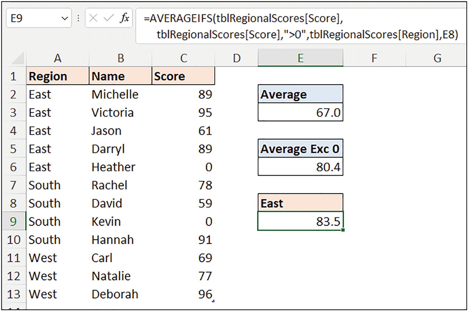
Average score for a specified region and excluding zero values
TRIMMEAN Function
Availability: All versions
trimmean.xlsx
The TRIMMEAN function returns the mean average for an array of values excluding a specified percentage of outlying values. It calculates the mean of the interior values of the array. The specified percentage of data is trimmed from the top and bottom ends of the array of values.
Array: The values to trim and average. This can be provided as a range, table column, or an array.
Percent: The percentage of values to exclude from the array. It can be entered into the function as a percentage or as a decimal value.
This percentage is taken in equal portion from the top and bottom ends of the array. So, for example, if there were 10 values and the percent was 20%, then 20% of 10 equals 2. So, one value would be excluded from the bottom and one value excluded from the top end of the array.

Average of all values in the [Total] column
Let’s trim this average with the TRIMMEAN function to exclude the outliers and return an average that is a better semblance of the data.

TRIMMEAN function excluding 20% of values
This returns the average of 406.40 – a better representation of the data. However, this TRIMMEAN function is only excluding one of the outlier values noted earlier.
There are 12 values in the [Total] column. 20% of 12 equals 2.4. This result is truncated to 2, so 2 values are excluded from the mean calculation.
Remember, the TRIMMEAN function trims from both ends of the array of values. So, the values of 11 (minimum) and 760 (maximum) are excluded from the mean calculation.
If we want to exclude the other outlier, the value of 27, then we will enter a larger percent in the TRIMMEAN function.

TRIMMEAN function excluding 35% of the values
This formula excluded both small outlier values and the two largest values in the column too.
We know this because 35% of 12 equals 4.2. This result is truncated to 4. So, TRIMMEAN trims the bottom 2 and top 2 values from the array. In this example, they are values 11, 27, 692, and 760.
Finally, a cell could be used as the input for the percent as an alternative to typing it directly into the formula. This would make it more dynamic and easily visible to those using the spreadsheet what percentage was used.

Using a cell as input for the percentage to trim
This is a small set of data (only 12 values) used for demonstration and to explain how TRIMMEAN works. In a larger array of values, 35% is a lot of values to exclude.
Conditional MEDIAN and MODE Functions
Availability: All versions
conditional-mode-and-median.xlsx
The average calculations so far have all been focusing on the mean average. Excel also contains functions to calculate the median and mode averages – fittingly named MEDIAN and MODE.
However, Excel does not have a conditional version of these functions like we have in AVERAGEIFS. So, we will create a formula by combining the MEDIAN or MODE function with the IF function.
Calculating the Median

Table of scores for median calculation
So, calculating the median may be a better average than the mean in this scenario.
The median is the middle number in a set of numbers. If there is an even set of numbers, MEDIAN will calculate the average of the middle two numbers.
But we want to create a conditional median formula. We want to know the median value for a specific region.
In this formula, the IF function tests the values in the [Region] column against the value in cell E7 and returns an array of all the corresponding values in the [Score] column where the test evaluated to True. This array was used by the MEDIAN function.

Combined with IF for a conditional MEDIAN formula
Other functions such as IFS, SWITCH, or CHOOSE could be used with the MEDIAN and MODE functions, instead of IF, to create the conditional element, especially if you have a more complex multiple condition scenario.
Calculating the Mode
The mode is the most common number in a set of numbers. In Excel, there are three mode functions – MODE, MODE.SNGL, and MODE.MULT.
The most used is the MODE function, but this was succeeded back in Excel 2007 by the MODE.SNGL function. MODE is only kept around for compatibility reasons; however, it is still the one most people use to this day.
The MODE functions only work with numeric values. In Chapter 11, when we discuss the INDEX and MATCH functions in Excel, we will see a technique to return the most frequent and least frequent text value.
Let’s focus on the two modern mode functions – MODE.SNGL and MODE.MULT. As you may have suspected, the SNGL stands for single and MULT stands for multiple.

MODE.SNGL function used to return the most common number

MODE.MULT returning the three most common numbers
If you are using a version of Excel that can natively handle arrays (Excel for Microsoft 365, Excel 2021, or Excel for the Web), then the three results are returned in a spilled array (covered in Chapter 10).
If you are using an older version of Excel, then you would need to select the three cells to store each of the returned numbers before writing the MODE.MULT function. Of course, this would mean that you would have to know that three answers would be returned. This makes the MODE.MULT function almost pointless to be used in this manner in older Excel versions.
Regardless of the version we are using, we may not want to return all three values. The MIN or MAX functions could be wrapped around MODE.MULT to return only the smallest or largest of the returned values.
This is a different behavior to MODE.SNGL, as that function returned the first of the three numbers to appear in the column.

Wrapping the MIN function around MODE.MULT
Now, let’s look at applying a condition to a mode function by including the brilliant IF function.

MODE.SNGL function with IF for a conditional mode formula
MAXIFS and MINIFS Functions
Availability: Excel 2019, Excel 2021, Excel for Microsoft 365, Excel for the Web, Excel 2019 for Mac, Excel 2021 for Mac, Excel for Microsoft 365 for Mac
maxifs-and-minifs.xlsx
Completing the IFS family of functions are the MAXIFS and MINIFS functions. They will return the largest and smallest numeric values in a list that meet one or more criteria.
They require the range of values to perform the maximum or minimum calculation on and the up to 127 criteria range and criteria pairs.

Table of scores from two different regions

MAXIFS and MINIFS functions returning results for the North
The MAXIFS and MINIFS functions can also be useful for analysis of dates. For example, the MAXIFS function will return the latest date in a range that meets specific criteria.
In Figure 8-48, we have a table named [tblWorkshops] that lists workshops and the date that they were held. We want to return the last date that each workshop was run. The MAXIFS function is perfect for this task.

MAXIFS function returning the latest date for each workshop
Using the Functions with Other Excel Features
ifs-other-features.xlsx
As always, we will conclude the chapter with some examples of how some of the functions in this chapter can be used with other Excel features. Let’s see examples with COUNTIFS and a use of the MEDIAN function.
Identifying Duplicates with Conditional Formatting
Working with duplicates is a common task for Excel users. So, it’s a good thing that Excel has many methods for tackling duplicates. These range from the Remove Duplicates and Advanced Filter features to using Power Query.
Instead of removing the duplicates though, we want to format them to make them easy to see when conducting further tasks.
Excel already has a built-in Conditional Formatting rule to highlight duplicate or unique values in a range. However, it is not as flexible as a custom rule that we can create ourselves with the COUNTIFS function.

Table of appointments that contains duplicate entries
- 1.
Select the cells in the data of the table, range B3:C16.
- 2.
Click Home ➤ Conditional Formatting ➤ New Rule ➤ Use a formula to determine which cells to format.
- 3.
Enter the following COUNTIFS formula into the Format values where this formula is true field (Figure 8-50):
- 4.
Click Format and choose the desired formatting to apply. Click OK.

Conditional Formatting rule to format duplicate entries
The formula counts the occurrences of each name in the range C3:C16 and returns True if the name occurs more than once. Conditional Formatting then applies the chosen format.
Range references are used in the COUNTIFS formula because Conditional Formatting does not accept a table’s structured references directly within a rule. However, if more names are added to the table, the COUNTIFS formula will automatically expand with the table.

Duplicate entries in a table formatted
Now, by writing our own formulas, we have greater control than the standard built-in rules that come with Excel. So, let’s say that we want to format the names that occur more than twice in the table. This is a more niche scenario of duplicate testing that goes beyond the built-in rules that Excel provides. This rule will be in addition to the previous rule.

Additional rule to identify names occurring more than twice
Incidentally, if you only wanted to format the second or third occurrence of the name, and not every instance of the name, edit the second half of the criteria range to have a relative row reference and begin from the first cell of the range. This creates a range that expands each row at a time.
Identifying Unmatched Values Between Two Lists
Earlier in the chapter, we saw the COUNTIFS function being used to compare two lists and flag the names that appeared in the first list but were missing from the second list.

Two lists to compare and highlight missing names
- 1.
Select the cells in the data of the first table, range B3:C16.
- 2.
Click Home ➤ Conditional Formatting ➤ New Rule ➤ Use a formula to determine which cells to format.
- 3.
Enter the following COUNTIFS formula into the Format values where this formula is true field (Figure 8-54):
- 4.
Click Format and choose the desired formatting to apply.
- 5.
Click OK.

COUNTIFS formula with NOT for unmatched values

Missing names identified in the first list
Highlight Values Larger Than the Median
The Conditional Formatting feature in Excel has built-in rules to highlight values that are above or below the average in the selected range (Figure 8-56).
These rules use the favored mean average just like the AVERAGE function of Excel. However, you may require the use of a different average calculation such as MEDIAN, TRIMMEAN, or MODE.

The standard above and below average Conditional Formatting rules

Table of scores
- 1.
Select the range of scores in the table, range C2:C16.
- 2.
Click Home ➤ Conditional Formatting ➤ Highlight Cells Rules ➤ Greater Than.
- 3.
Enter the following formula into the Format cells that are GREATER THAN box provided (Figure 8-58):

Format cells greater than the median value
- 4.
Specify the format you want to apply from the drop-down list.
- 5.
Click OK.

All scores greater than the median are highlighted
Preventing Duplicate Entries
For the final example, let’s go back to working with duplicate values. This time though, we will use the Data Validation tool with COUNTIFS to prevent duplicate entries in a list.
In Figure 8-60, we have a simple list of countries. We will create a validation rule to prevent the same country from being entered more than once.

Table with country names
- 1.
Select the range of countries, range B3:B6.
- 2.
Click Data ➤ Data Validation.
- 3.
On the Settings tab, select Custom from the Allow list and enter the following formula into the Formula box (Figure 8-61):

COUNTIFS formula in a Data Validation rule
- 4.
Click the Error Alert tab and enter a meaningful error for an invalid entry.
- 5.
Click OK .

Duplicate country detected and error alert shown
Summary
In this chapter, we learned functions that perform aggregations dependent upon conditions that are met. These included SUMIFS, COUNTIFS, and combining functions such as MEDIAN with IF.
We learned some cool tricks to apply with these functions, for example, using OR logic with SUMIFS and creating conditional rankings with COUNTIFS.
In the next chapter, we will look at two functions that take it to the next level in aggregating data – SUMPRODUCT and AGGREGATE. These functions are incredible, and each one has a special set of abilities that makes it so useful. Let’s dig in.