
One of the most important skills to learn in Excel is understanding how to reference values and arrays. Whatever you use Excel for, you need to know how to specify the location of a value or array. One could argue that it is the most important skill.
This does not just apply to formulas, but charts, PivotTables, formatting, validation rules, etc. It all boils down to being able to tell Excel the locations of the values or array that you need.
Data could be stored on the grid, in a table, a defined name, a spill range, an array returned by a formula, or stored as a date type (covered in Chapter 14). There are so many options, and this is partly what makes Excel so exciting.
There are many lookup and reference functions in Excel, and these functions provide us with the means to access the values and arrays in the manner we require.
We covered the VLOOKUP function in Chapter 7. It has its own chapter in this book due to its overwhelming popularity as a function. But Excel has so many more functions that extend beyond the capabilities of VLOOKUP. Therefore, the chapter has been coined “Advanced Lookup Functions.”
We will cover many of the most useful lookup and reference functions in this chapter. There will be dedicated chapters for the new XLOOKUP and FILTER functions to follow this one. These are two of the finest lookup and reference functions in Excel.
In this chapter, we will cover the CHOOSE, INDIRECT, OFFSET, VSTACK, and XMATCH functions, to name just a few. The INDEX function is also covered and deserves a special mention independently from the others as it is possibly the best function in Excel.
MATCH Function
Availability: All versions
match.xlsx
The MATCH function is one that we will see a lot of in this chapter. It is a real workhorse that performs a lot of the legwork for other lookup functions to perform dynamic relative references.
Lookup value: The value you want to look for and return its relative position.
Lookup array: The range or array to search in for the lookup value. This can be a vertical or horizontal array.
- [Match type]: The number 1, 0, or –1 that defines the match type.
0 is entered to specify an exact match. This is the most used match type.
1 is entered to perform a range lookup that returns the position of the largest value less than the lookup value, if the lookup value is not found. The lookup array must be sorted in ascending order when using this match type. This is also the default match type.
–1 is entered to perform a range lookup that returns the position of the smallest value greater than the lookup value, if the lookup value is not found. The lookup array must be sorted in descending order when using this match type.
The MATCH function is case-insensitive. It does not distinguish between lowercase, proper case, and uppercase when matching text values.

Simple MATCH example returning the relative position of a name
If the lookup array contains duplicate values, the MATCH function will return the position of the first occurrence of the value that it finds.

#N/A error returned when a value is not matched
Let’s look at some more practical examples of the MATCH function in action. There are further examples of MATCH throughout this chapter, especially when combined with the INDEX function, its most familiar partner.
Compare Two Lists
The MATCH function provides a neat way to compare two lists and identify the differences.
When comparing two lists, if a value is matched, its relative position is returned; otherwise, the #N/A error is returned.

MATCH function comparing lists for matching values
You can see that there are three names in the first table that are not matched in the second table. This is shown by the #N/A error message.
Although this works, it is not a very polished result.
The MATCH function can be nested within other functions to display an alternative value or to perform an action based on the result. It could also be inserted into a Conditional Formatting rule to visualize the differences between the two lists better.

Tidying up the results to display “Yes” and “No” values
Dynamic Column Index Number in VLOOKUP
We covered the VLOOKUP function in Chapter 7 in great detail, including tricks for returning the column index number as an alternative to typing in the column number directly.
The MATCH function is a terrific method for fetching the column index number for VLOOKUP. It provides an approach that is robust, durable, and dynamic.
We will use the MATCH function to search for the header text of the column we want, along the header row of the lookup table, and return the relative position of that column to VLOOKUP.
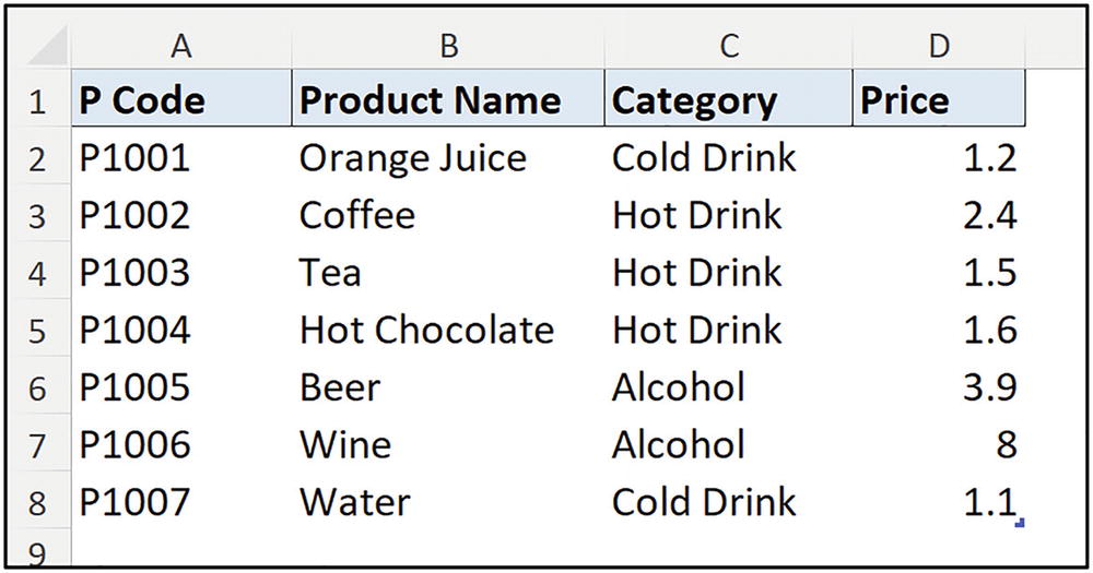
Table of product data
The MATCH function searches the header row of [tblProducts] to return the column number of the header stated in cell D1. The header text of the value in cell D1 and that in the lookup array must match exactly.
Notice the absolute reference to the P Code lookup value. This technique was covered in Chapter 4, when we covered tables in detail. Also, the row has been made absolute in the reference to the header text in cell D1.
These references have been applied so that the VLOOKUP formula can be filled across the [Category] and [Price] columns too.

Returning product details with VLOOKUP and MATCH
Sort a Range by Drop-Down List Value
Using the MATCH function combined with the SORT function, we can create a nice effect for our Excel reports and models, where a user can sort a range by selecting the column to sort by from a drop-down list.
This is a great technique, as it makes our reports interactive from functionality on the grid, instead of a user having to know how to use built-in Excel features. It also gives us more control to setting up how a feature of a report should be used.
The SORT function requires that the column to sort by is entered as an index number. This is a perfect scenario for the MATCH function to assist.
Figure 11-7 shows a table named [tblCoffee] that contains aggregated sales data for six different products.

Table with data about coffee sales
The same MATCH function is used twice in the formula. The first MATCH is used to return the sort index. It matches the text in cell B2 to the headers in [tblCoffee] and returns the column number.
The second time the MATCH function is used is within an IF function. The IF function is used here to ensure that the correct sort order is applied.

Sorting table data based on drop-down list selection
To avoid the repetition of the same MATCH function in one formula, we could define a name for the MATCH function and use that name in the formula instead. This would help us to create a more meaningful and concise formula.
- 1.
Click Formulas ➤ Define Name.
- 2.
Type “SelectedColumn” for the Name (Figure 11-9).
- 3.
Enter, or copy, the MATCH formula into the Refers to box. Click OK.

Named formula for the MATCH function
This formula is much more concise and meaningful.
In Chapter 15, we cover the LET function in Excel. With LET, we can save variables with meaningful names and repurpose them within a formula. Using LET prevents us from having to define named formulas like we did here for this example.
XMATCH Function
Availability: Excel 2021, Excel for Microsoft 365, Excel for the Web, Excel 2021 for Mac, Excel for Microsoft 365 for Mac
xmatch.xlsx
The XMATCH function is the successor to the MATCH function and offers a few refinements and added functionality over its predecessor. It is only available in the 365, Online, and 2021 versions of Excel though, so MATCH is still very important to know.
The key changes with XMATCH are that it defaults to an exact match type and that it has the ability to search an array from first to last or from last to first.
Lookup value: The value you want to look for and return its relative position.
Lookup array: The range or array to search in for the lookup value. This can be a vertical or horizontal array.
- [Match mode]: The number –1, 0, 1, or 2 that defines the match type.
0 is entered to specify an exact match. This is the most used match type and the default option.
–1 is entered to return the position of the exact match or the next smaller value to the lookup value, if the lookup value is not found.
1 is entered to return the position of the exact match or the next larger value to the lookup value, if the lookup value is not found.
2 is entered to specify a wildcard character match. The asterisk (*), question mark (?), and tilde (~) wildcard characters can be used for partial matches.
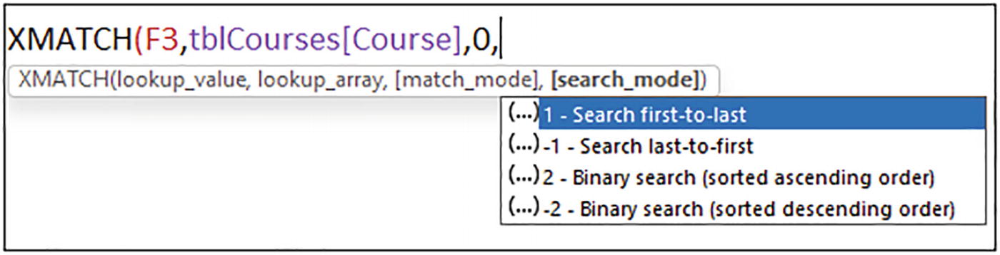
- [Search mode]: The number 1, –1, 2, or –2 that defines the type of search to perform.
1 is entered to specify a search from first to last. This is the default search mode.
–1 is entered to reverse the search and search from last to first.
2 is entered to specify a binary search from first to last. Performing this type of search requires the lookup array to be sorted in ascending order.
–2 is entered to specify a binary search from last to first. The lookup array needs to be sorted in descending order for this type of search.
The numbers used to specify the “next item smaller than” and “next item larger than” match modes are the reverse of the numbers used by MATCH. Be careful with this change when you start using XMATCH.
Because we have covered the MATCH function already, the following examples will focus on highlighting the differences between XMATCH and MATCH.
XMATCH Defaults to an Exact Match
The most used match type is the exact match, and this is the default match type of XMATCH, unlike the MATCH function. So, when performing an exact match, we do not need to answer the third argument.

XMATCH function defaults to exact match
Returning the Position of the Last Match
The search mode argument of the XMATCH function provides the ability to search an array from last to first. This is useful for returning the position of the last match in an array.

Rounds of results for different teams
In Figure 11-12, the XMATCH function has been used to return the round that a team recorded their first win and the number of rounds it has been since their last win.
To return the number of rounds since a team won their last match, we need to return the relative position of the last match of a “W.”

Returning the number of rounds since the last win
We will see further examples of the XMATCH function and showcase other uses of its arguments when we discuss the INDEX function later in this chapter.
CHOOSE Function
Availability: All versions
choose.xlsx
The CHOOSE function is a simple yet very effective function in Excel. It chooses a value, range, or an action from a list based on an index number.
We have seen a few examples of the CHOOSE function in this book so far. It has been demonstrated in Chapters 6, 7, and 10. It was used to return fiscal quarters from dates in Chapter 6. And in Chapters 7 and 10, it was used to reorder or extract specific columns for the VLOOKUP and SORT functions.
It is a very useful function in Excel, so in this chapter we will see some further examples of its use.
Index num: The index number of the value, range, or action in the list that you want to use
Value, [value 2]: The list of values, ranges, and actions that you want to return from

Simple CHOOSE function
The true power of the CHOOSE function is revealed when the index number is provided by the result of a formula or via a form control. So, let’s take the CHOOSE function further.
Generating Random Sample Data
CHOOSE is great for generating random sample data that can be used for testing formulas and models that you create. In fact, much of the sample data provided in this book was generated using these methods.
The RANDARRAY function returns an array containing ten rows of integer values between 1 and 3. The CHOOSE function returns the region from its list based on the index number provided by RANDARRAY and spills the results to the grid.
The RANDBETWEEN function can be used instead of RANDARRAY in Excel versions that do not support the RANDARRAY function.

Generating text values at random
Remember, when using the random number–generating functions – RAND, RANDBETWEEN, and RANDARRAY – they return new results every time the worksheet calculates.
- 1.
Select the range you want to convert to values.
- 2.
Position the cursor on the border of the selection until you see the “move” cursor (four arrows facing away from the center).
- 3.
Right-click and drag away and then back to the range and release the mouse.
- 4.
Click Copy Here as Values Only (Figure 11-15).

Converting formulas to values only
To complete the sample data, we will generate random values for the [ID], [Date], and [Total] columns. We will not be using the CHOOSE function for this task, despite it being the focus of this part of the chapter, but it is important to finish the job.

SEQUENCE generating a series of ID values
The DATE function is used in the min and max arguments of RANDARRAY to specify the start and end dates of the date range. The SORT function is added to order the dates returned in an ascending order.
Instead of adding the SORT function, we could have generated the dates before generating the ID values and sorted the dates manually using the commands in Excel.

Random date values in July 2021 in ascending order

Generating random decimal values
Return a Range Based on a Cell Value
In this example, we want to return a range dependent upon the value selected from a drop-down list.

Data for range selection by CHOOSE
When a different location is chosen in cell C4, the formula returns the required results.
In a dynamic array version of Excel, the results of this formula are spilled to the cells below.
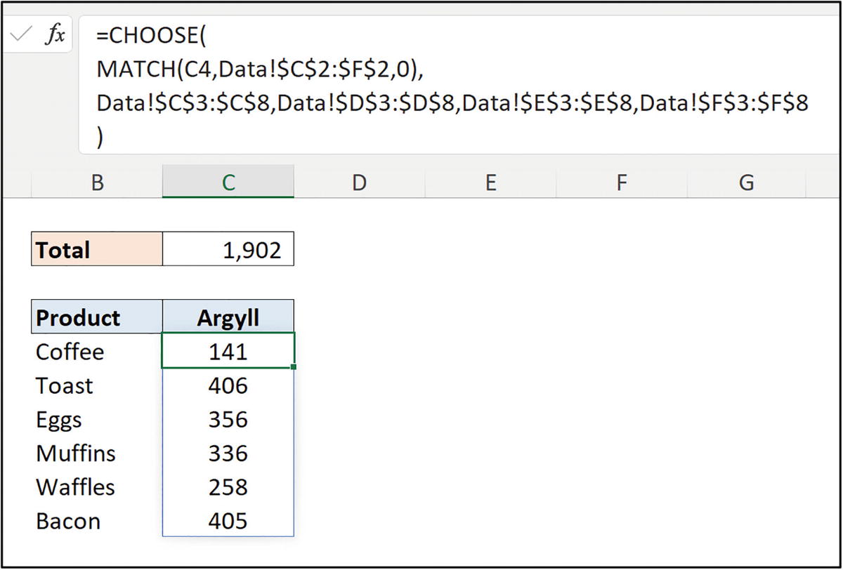
Returning a range based on the value in cell C4
Sure! In this example, the total could have been produced by referencing the range in C5:C10. In a dynamic array version of Excel, the spill range could be used, =SUM(C5#), but in other versions the fixed range could be used, =SUM(C5:C10).
However, we wanted to demonstrate the use of the CHOOSE function returning a range based on a cell value and passing this directly to the SUM function. This formula would sum the values for the chosen location without the need to return the values to the worksheet.
Choosing a Function from a List
The technique of selecting a different function from a list is one of my favorite uses of the CHOOSE function. The list can contain any functions you want. In this example, the SUM, AVERAGE, and MAX functions are made available for a user to choose from.
In Figure 11-21, there is a drop-down list in cell B2, so the user can easily select the function they want to use. The table of product names and total values is named [tblSales].

Choosing a function from a drop-down list
Simple and very effective. We have seen in the examples so far how easily the CHOOSE function can be used to insert some interactivity into an Excel report or model, and how a user could change the calculation being applied or the range that is being used.
Using CHOOSE with Form Controls
A few of the form controls in Excel, such as the list box, combo box, and option buttons, return an index number to represent the selection made in the control. This makes them ideal to be used with the CHOOSE function, as CHOOSE also uses an index number to identify the selection made.
Continuing with the previous example, let’s provide a form control for the user to make the function selection instead of the drop-down list. We will use the option button control for the example.
Figure 11-22 shows three option buttons, one for each of the three functions to choose from – SUM, AVERAGE, and MAX. The table of product names and totals is named [tblProductSales].

Option buttons to enable the user selection of a function
- 1.
Click Developer ➤ Insert ➤ Option Button (Form Control) (Figure 11-23).
Note No Developer tab on the Ribbon? Right-click the Ribbon, click Customize the Ribbon and check the Developer box in the list on the right. Click OK. On a Mac, click Excel ➤ Preferences ➤ Ribbon & Toolbar ➤ Customize the Ribbon and check Developer.

Inserting an option button form control
- 2.
Right-click the option button and click Edit Text. Replace the existing text with the name of the function, that is, Sum.
- 3.
Repeat steps 1 and 2 for each option button.
- 4.
With an option button selected, click Developer ➤ Properties.
- 5.
On the Control tab of the Format Control window (Figure 11-24), click in the Cell link box and click the cell you want to connect the option button with. Click OK.
Cell F1 has been used in this example. This means that the index number of the selected option button will appear in this cell.
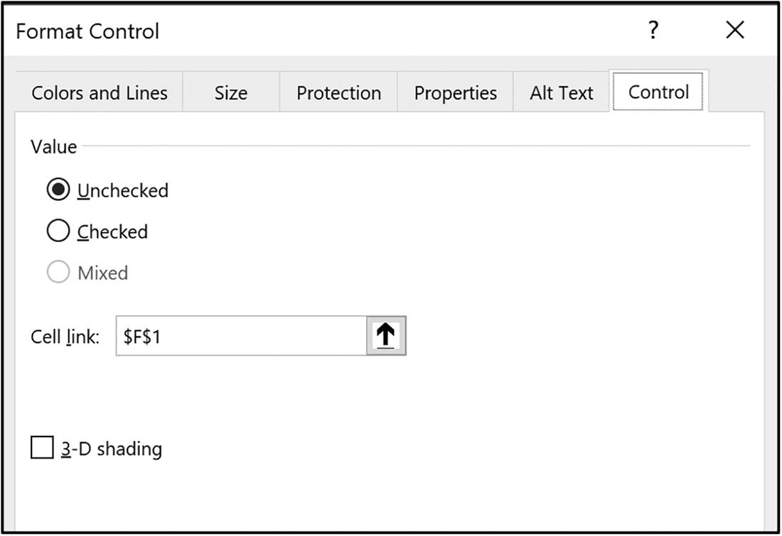
Formatting the option button controls
Now that we have our option button controls inserted, let’s get back to the CHOOSE function.
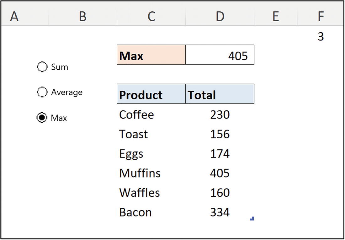
Choosing a function via option buttons
INDIRECT Function
Availability: All versions
indirect.xlsx
The INDIRECT function converts a text string into a reference to a cell, table, named range, or some other reference.
It is used to create dynamic references within formulas. Instead of directly typing a reference into a formula, a cell value can be used as the input of the reference text. The reference within the formula is then updated when the cell value is changed.
Ref text: The reference to a cell, range name, or table entered as text.
[a1]: A logical value that specifies the type of reference to be used – A1 or R1C1. Enter TRUE or omit the argument to specify the A1 reference style. Enter FALSE for the R1C1 reference style.
When using INDIRECT, the A1 style is generally used; therefore, the second argument is normally omitted. The A1 style is the style that Excel users are more familiar with. For example, B3 and D10 are both A1 style references.
An R1C1 reference style is when numbers are used to reference the row and column of a cell. It is always entered with the row first and the column second. For example, R4C5 is a reference to cell E4. Cell E4 is in the fourth row and the fifth column.
INDIRECT is one of the eight volatile functions in Excel. These functions recalculate, along with all dependents, every time Excel recalculates. Heavy reliance on these functions can slow calculation time, so should be used sparingly. Worth knowing, however it does not detract from INDIRECT being very useful.
To demonstrate a simple example of how INDIRECT works, in Figure 11-26, cell D2 indirectly references cell B2.

Basic example of INDIRECT
Let’s see some more practical examples of the application of the INDIRECT function. We will see examples that demonstrate the dynamic referencing of ranges on other worksheets, named ranges, and data stored in tables.
Indirect Table Reference in VLOOKUP
In this first example, we will use the INDIRECT function to indirectly reference a table.
We want to use the VLOOKUP function to return the grade associated with the score a student achieved in a subject. Each subject has its own grading system, so they have their own separate lookup tables. VLOOKUP will know which lookup table to refer to because it is specified in a cell. INDIRECT will perform the task of converting this cell value into a reference for VLOOKUP.

Lookup tables for different subjects

VLOOKUP indirectly referencing a table
Referencing Table Columns with INDIRECT
In this example, instead of referencing an entire table we will reference a specific column within a table.
We have four tables, each containing sales data for a different city – [tblManchester], [tblLeeds], [tblPlymouth], and [tblLincoln]. We want to use the SUM function to sum values from the table specified by a cell value.
Figure 11-29 shows the four different tables. We want to sum the values in the [Total] column for the specified table. To do this, we need to build a reference from some text strings and a cell value in INDIRECT.

Separate tables for different cities

INDIRECT to reference a table column
Referencing Other Worksheets
The INDIRECT function can be used to dynamically reference other worksheets using the value in a cell.

Sales data on separate worksheets
Within the INDIRECT function, the reference to the sum range is made up of three parts. There is a single quotation ('), followed by the value in cell B3, and then the final string. The final text string contains the closing single quotation, an exclamation mark, and then range C3:C7.
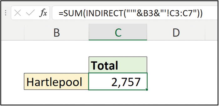
INDIRECT to reference a sheet using a cell value
When the sheet name in cell B3 is changed, the formula updates to sum the correct values.
In Chapter 1, we covered the topic of sheet references. If any aspect of the references is unclear, I encourage reading through that chapter and the dedicated chapters for defined names and working with tables. A strong understanding of how to reference cells is imperative for advanced formula skills.
Pivot Style Report with Dynamic Row Labels
We have created a couple of pivot style reports in this book using dynamic array formulas. In this example, we take it further by using the INDIRECT function to create dynamic row labels. The example uses dynamic arrays and so requires an Excel for the Web, Excel for Microsoft 365, or Excel 2021 version of Excel.
The report will be created using the table shown in Figure 11-33. This table is named [tblSales]. The image shows a snapshot of the first nine rows of the table.
For the pivot style report, we will display the last N months along the column labels using the SEQUENCE formula on the [Date] column that we detailed in Chapter 10.
For the row labels, we will provide a drop-down list for the user to pick between the [Sales Rep] column and the [Region] column. The INDIRECT function will be used to create the functionality for a user to switch between columns via a drop-down list.

Sales data for the pivot style report
Figure 11-34 shows the setup of the pivot style report before we introduce the dynamic row labels and sales totals.

Drop-down list to pick the column to use for row labels
To create the dynamic row labels, we will create a distinct list for each of the [Sales Rep] and [Region] column values using dynamic array formulas. We will then define names for these spill ranges and use the INDIRECT function to dynamically refer to these names.

Lists for the sales reps and region labels
In Figure 11-36, the Name Manager shows the two defined names established for each spill range.
The [Sales_Rep] name has been defined for the “Sales Rep” value in the drop-down list. You cannot use spaces in a name, so the underscore was used as the delimiter.
Unsure how to define a named range? Please refer to Chapter 3, where we learn all about defined names in Excel.

Defined names for the two list spill ranges
This formula refers to the table column using a reference that is a combination of text strings and the value in cell C4, like we covered a couple of examples previously.
Dynamic row labels with INDIRECT
In the criteria range 1 argument of SUMIFS, the INDIRECT function is used to refer to the correct table column as stated in cell C4.

Dynamic SUMIFS added to complete the pivot style report
R1C1 Reference with INDIRECT
In addition to the A1 style of reference generally used with INDIRECT, the R1C1 reference style can also be applied. With the R1C1 style, row and column numbers are used to specify the cell reference. This is especially useful for columns as the A1 style does not enable us to refer to a column using a number.
A MATCH function is used to return the row number of the name specified in cell B2. The R1C1 reference of INDIRECT refers to the row and column numbers of the sheet, so four is added to this value to offset the four rows above the names in the table (B1:B4).
The COLUMNS function is used to return the number of columns in the [tblMonthly] table. One is added to account for column A to the left of the table.

R1C1 reference style used with INDIRECT
The INDIRECT function can also be used to return a range.
In this formula, two INDIRECT functions using R1C1 reference styles are used to form a range by entering a colon (:) between them. This is given to a SUM function to sum the values.
The first INDIRECT is fixed to start from column 3, while the second INDIRECT returns the final column in the table using the COLUMNS function with one added to it. MATCH is again used to return the row number for the name entered in cell B2.
The INDEX function is a better function for referring to cells using numbers. This example of an R1C1 reference style is only shown for the purposes of a deeper understanding of the INDIRECT function.
OFFSET Function
Availability: All versions
offset.xlsx
The OFFSET function returns a reference to a range that is a given number of rows and/or columns from a start range. This reference can be a single cell or multiple cells that are a specified number of rows high and columns wide.
This function is fantastic for dynamic references that may change in size over time or are specified by the value in a cell.
Reference: The start reference from which to offset.
Rows: The number of rows above or below the start reference you want to offset. Enter a positive number to reference the range the given number of rows below, or a negative number to reference the range the given number of rows above.
Cols: The number of columns to the right or left of the start reference you want to offset. Enter a positive number to reference the range the given number of columns to the right, or a negative number to reference the range the given number of columns to the left.
[Height]: The number of rows in height of the returned range. This is an optional argument, and if omitted, the range returned is the same height as the start reference.
[Width]: The number of columns in width of the returned range. This is an optional argument, and if omitted, the range returned is the same width as the start reference.
The OFFSET function gets a somewhat unfair reputation of being bad due to it being a volatile function. This means it recalculates every time Excel recalculates, regardless of which cell values were changed. It is, however, a very useful function that should not be disregarded so easily.
Simple Examples
Let’s begin by looking at some simple examples of OFFSET to get a strong understanding of how it operates before we progress to more practical examples.

Simple OFFSET example
Functions such as COUNT, MATCH, and COLUMNS are often used to calculate the number of rows or columns to offset. So, let’s see an example.
The start reference is G4. This is the top-left corner of the range that we are returning the value. This start reference can be any reference. However, it is often the top-left corner cell of the range or table from which you are returning the reference.
The MATCH function is used to find the number of rows to offset, and an input cell (H2) is used for the number of columns to offset.

OFFSET example using cell values for row and column offsets
Sum the Values in the Nth Column
The OFFSET function can return a range of cells, and this range can be given to another function for use. This delivers the ability to provide dynamic ranges to functions.
The start reference is cell B5, so the range to return is offset by one row. If the OFFSET function was given a start reference of B6 (same row that the numbers start), we would not need to offset a row. However, it is important to be consistent in the way you work, and I like to use the top-left corner cell. The number of columns to offset is specified by the value in cell B3.
The ROWS function is used to ascertain the height of the range to return. The ROWS function returns the number of rows in the table, excluding the headers.

Summing all values for a specified column
The cell input being provided may be the month name instead of the month number. This is no problem, as a function such as MATCH can be used.
One is subtracted from the result returned by MATCH. This is because the MATCH function is searching for the matching month name in all headers of the table. And because the start reference is in the first column of the table, MATCH returns a column number one more than is required.
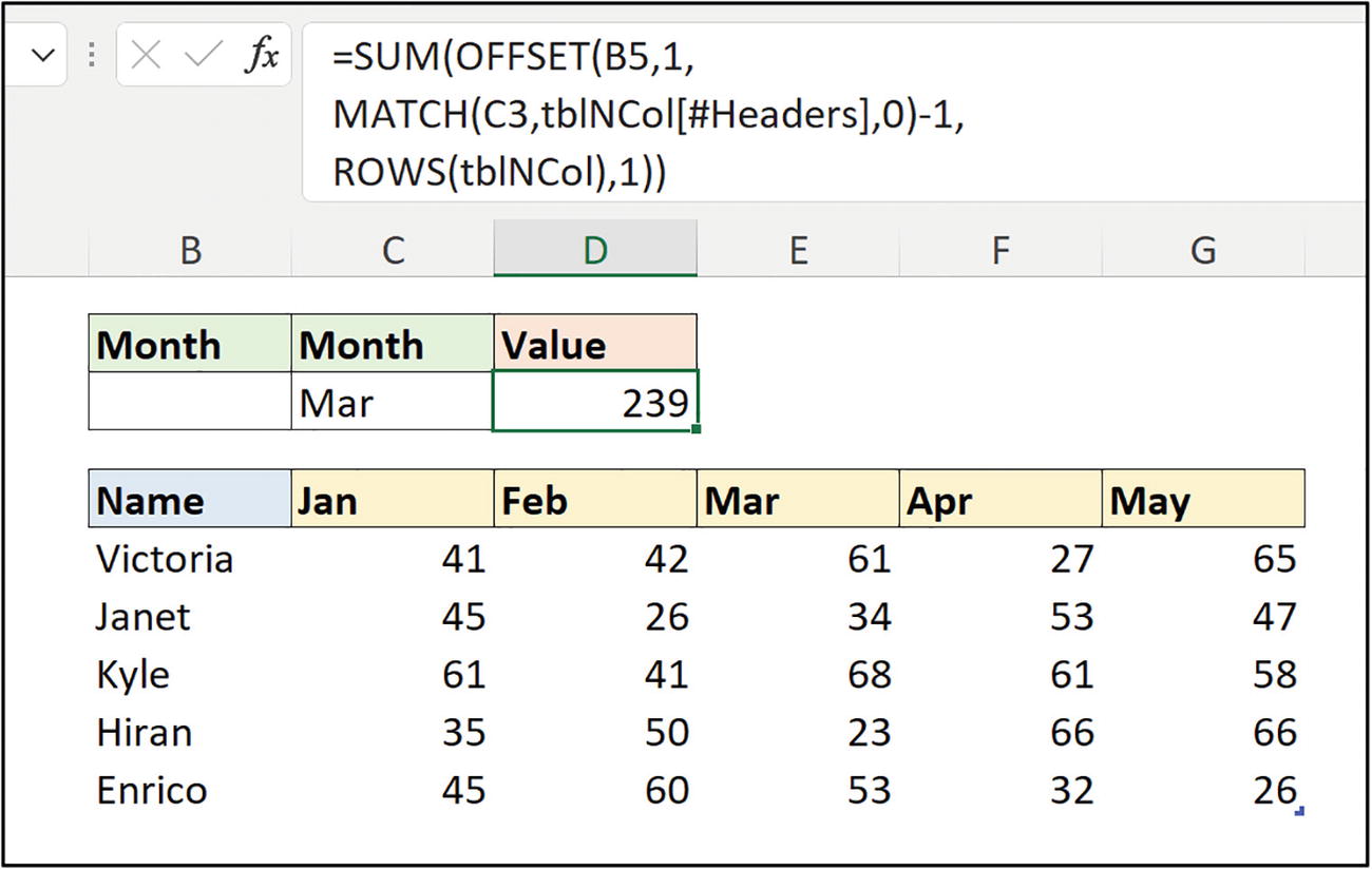
Summing the values of a specified column with MATCH

Summing all values in the last column of a table
Return the Last X Columns
Instead of returning a range to another function, it could be returned to the worksheet.

Table of team results
From another sheet, we want to return the last six results for a specified team. It is common in sports dashboards to see recent results for teams like this.
The COLUMNS function is used to find the starting column. COLUMNS returns the number of columns in the table, and six is then subtracted from this result to return the correct number of columns to offset.

Returning the last six results for a specified team
These formulas are being demonstrated in a dynamic array–enabled version of Excel. In non-dynamic array–enabled versions of Excel, the range of cells to return the reference will need to be selected before typing the formula. Also, Ctrl + Shift + Enter needs to be pressed to run an array formula.
The start reference used in both formulas is a reference to cell B2 of the [Results] worksheet. This is the cell in the top-left corner of the table. This works great, but an alternative approach could be to refer to the table itself.
The OFFSET function returns a reference with the same dimensions as the start reference if the height and width arguments are not stated. This is important to remember if you are going to use multiple cell start references.
OFFSET with COUNTIFS
The OFFSET function can be used to provide a range to any function that requests one. We have seen an example of this already with the SUM function. Let’s use the formula from this example with the COUNTIFS function to return the number of wins for a specific team in the last X number of rounds.

OFFSET with COUNTIFS to count number of wins
This same technique can be applied to return the last X rows in a range by applying the ROWS function instead of COLUMNS, for example, to sum the last X rows.
INDEX Function
Availability: All versions
index.xlsx
The INDEX function is an absolutely incredible function in Excel. It does not sound very sexy, but it is stunningly useful. This section of the book will run through numerous examples that demonstrate the amazing power and versatility of this function.
The INDEX function is often teamed up with the MATCH or XMATCH function to create a flexible lookup formula. You may have heard of or used an INDEX-MATCH combination before.
The usefulness of the INDEX function stretches far beyond its role in the INDEX-MATCH combo. And in modern versions of Excel, with the dynamic array formulas, applications of INDEX have broadened even further. It is better and more important to know than ever before.
Introduction to the INDEX Function
The power of the INDEX function is really down to its simplicity and flexibility. The role of the INDEX function is to return the value or reference of a cell from a specified row and column number, in a given range.
A key part of that INDEX function description was its ability to return a value or a reference. It is incredibly helpful in accessing values in ranges, arrays, and spill ranges, but also creating dynamic references for other formulas or Excel features such as charts.
The description also stated that we need to provide the row and column number from which it returns the value or reference. This indexing approach is its superpower. We can state the row and column number in an absolute manner or find them using another function such as MATCH, COLUMN, COUNTA, and so on.
The sky is the limit for the INDEX function.

The two syntaxes of the INDEX function
Array: The range or array from which to return the value or reference.
Row num: The row number in the array from which to return the value or reference. This argument is optional. If omitted, a column number should be provided.
[Column Num]: The column number in the array from which to return the value or reference. If omitted, a row number should be provided.
When using the INDEX function, you will nearly always be using the first syntax. It is only the final INDEX function example in this book that demonstrates a use of the second syntax.
Reference: This is a list of one or more references enclosed within brackets.
Row Num: The row number in the chosen reference from which to return the value or reference. This is an optional argument.
[Column num]: The column number in the chosen reference from which to return the value or reference. This is an optional argument.
[Area num]: The index number of the reference you want to return from the list of references.
Basics of the INDEX Function
To get a solid understanding of how the INDEX function operates, we will start with some basic examples and progress to the more exciting stuff.

Simple INDEX example
An interesting aspect of the INDEX function is that it returns the values or reference of all cells in a row or column, if a row or column number is omitted.
This is very useful for users with a dynamic array–enabled version of Excel. It is a powerful method to access elements of an array. And we will see this technique later in this “INDEX Function” section and again later in the book.
Let’s see exactly what I mean by this using the same range of B3:C8.

Returning all values in the row by omitting the column number

Returning all values in a column by omitting the row number
In all the examples so far, the column and row numbers have been entered directly into the formula. These numbers are normally returned by a function such as MATCH, COLUMNS, ROWS, or COUNTA for a dynamic and more robust method. Form controls such as the list box and option buttons are also great for serving index numbers to the INDEX function.
The most popular function to be affiliated with INDEX is the MATCH function. And in modern versions of Excel, it is the XMATCH function. With these functions, we can return the row or column number that matches a value we are looking for.
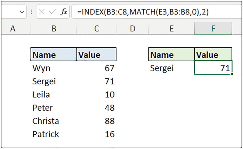
INDEX and MATCH functions to look up a specific value
This example uses a sheet range for the array that INDEX returns from and for the lookup array that MATCH searches in. This is adequate, but using data formatted as a table is more commonplace and provides additional advantages. Therefore, many, though not all, forthcoming examples will be working with data formatted as a table or an array returned by another function.
INDEX and MATCH/XMATCH for Versatile Lookups
Let’s continue with further examples of the fantastic combination of INDEX and MATCH or INDEX and XMATCH functions. Together they provide an extremely versatile lookup formula that is available to all versions of Excel.
We saw a workaround in Chapter 7 that used the CHOOSE function to enable VLOOKUP to return a value from a column to the left of the lookup column. Now, the better alternative to that approach is the INDEX and MATCH combination. And these functions are available in all versions of Excel, unlike the newer XLOOKUP and FILTER options.
With INDEX and MATCH, you can look for a value down any column of a range or table (VLOOKUP only looks down the first column) and return from any column of the range or table.
INDEX and MATCH will also look along and return from data arranged in rows, and we will see examples of this shortly.
In Figure 11-53, we have two tables. The table on the right is named [tblGrades]. It contains four different grades, each one associated with achieving a particular score. This is the lookup table, and notice that the [Grade] column is to the left of the [Score] column.
The table on the left is named [tblScores] and contains the scores achieved by different people.
This formula demonstrates the versatility of INDEX and MATCH. It makes it simple to look for and return a value from any column of a table. It also highlights that INDEX-MATCH works brilliantly with data formatted as a table.

Versatile INDEX and MATCH returning from a column to the left

INDEX and XMATCH performing a versatile range lookup
Two-Way Lookup with INDEX and MATCH/XMATCH
A two-way lookup can be created by using two MATCH or XMATCH functions with INDEX – one to search for a value down a column and another to search along a row.
Figure 11-55 shows a matrix of data. It contains prices for different holiday accommodations. The price is dependent upon the type of accommodation and the location. The type of accommodation is labeled in range B3:B7, and the different locations are labeled along range C2:F2.
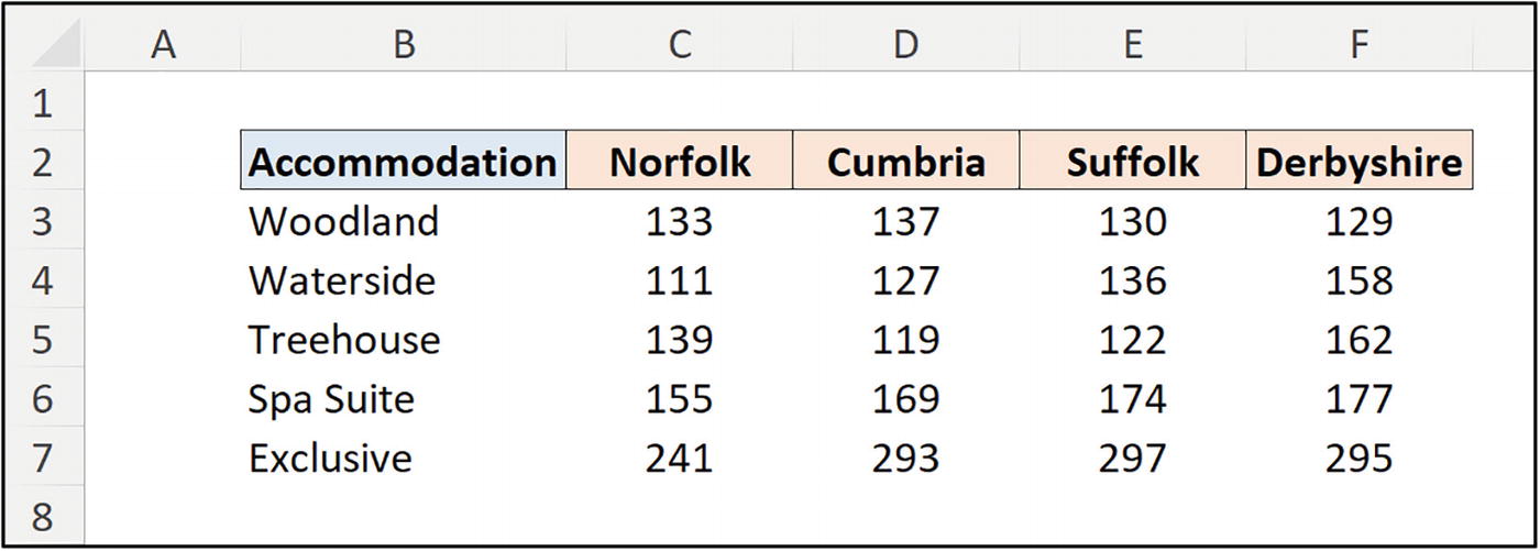
Data matrix of accommodation prices by location
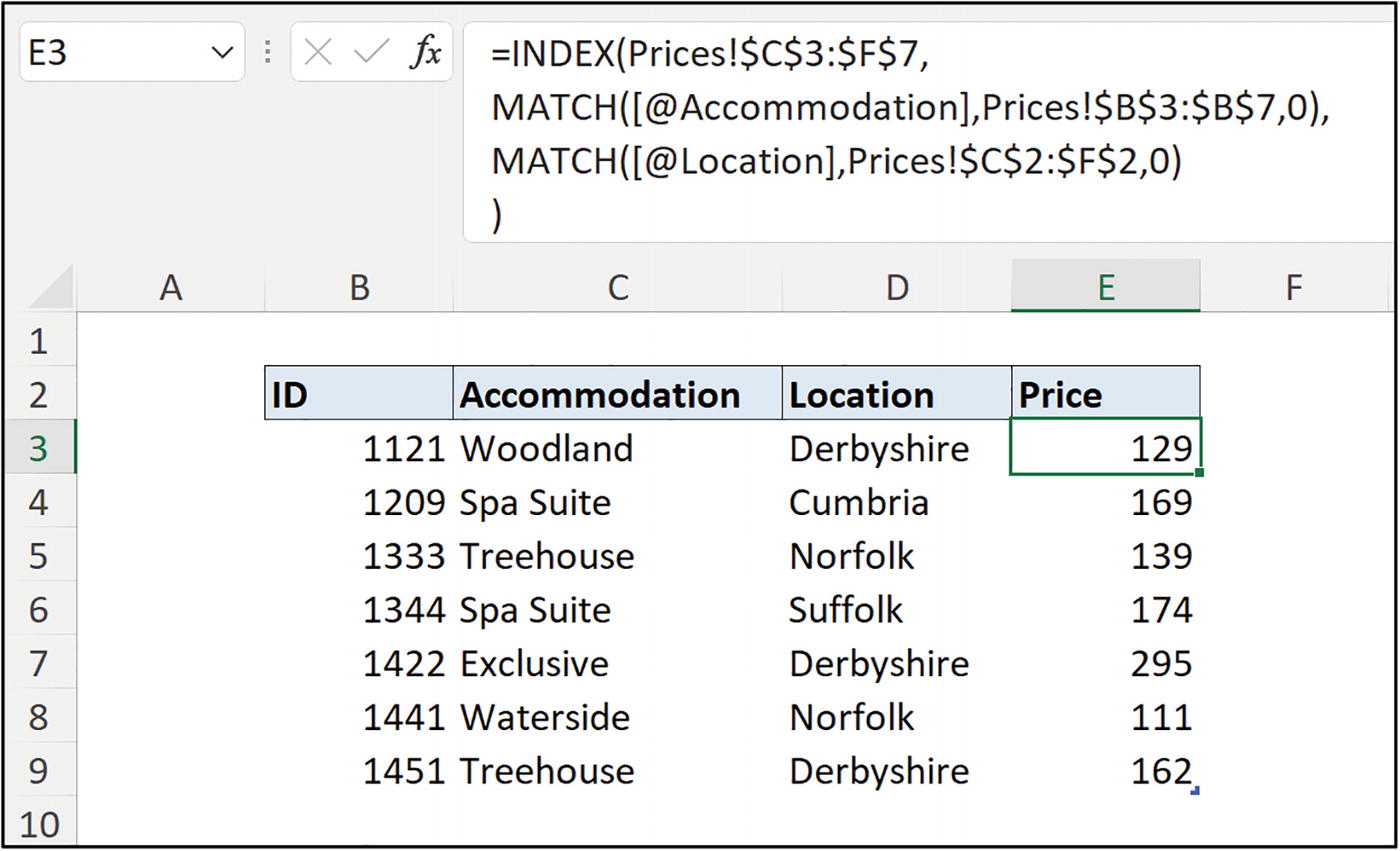
Two-way lookup with INDEX and MATCH
It is important in this formula that the array given to INDEX is the same height as the vertical lookup array and the same width as the horizontal lookup array given to the MATCH functions.
Using Wildcards with INDEX and MATCH/XMATCH
The MATCH function will handle wildcard characters natively. This makes it simple to perform partial text matches with the INDEX and MATCH combination. With the XMATCH function however, a wildcard character match needs to be specified.

Table of target values by city
We need to perform a lookup using the city name only, so will perform a partial match for any value that begins with the city we are looking for.
* (Asterisk): Represents any number of characters. For example, New* would match with Newport, Newcastle, New York, and New Zealand.
? (Question mark): Represents a single character. For example, L????n would match with both London and Lisbon.
~ (Tilde): Used to treat a wildcard character as a text character. For example, *don would match any text that ends in the characters don, but ~*don will look for an exact match of *don, treating the asterisk as its character and not a wildcard.

Using wildcard characters with INDEX and MATCH
Last Occurrence of a Value with XMATCH
One of the advantages that XMATCH has over MATCH is the ability to search an array from last to first. By searching from last to first, XMATCH can be used to return a value relating to the last match in a row or column.
Search mode option in the XMATCH function
In Figure 11-60, the INDEX and XMATCH combination is used in cells G3 and H3 to return the date and number of attendees for the last occurrence of the training course entered in cell F3.

INDEX and XMATCH for the last match in column
Let’s see another example. This time, we will use INDEX and XMATCH to search both down a column and along a row.
Figure 11-61 shows the results of 12 rounds of games for six different teams. The teams are listed down column B and the results arranged along rows. “W” represents a win, “D” is a draw, and an “L” is a loss.

Team results over 12 rounds of games
There is a nested INDEX and XMATCH in this formula to return all results for the team name entered in the corresponding row of range B3:B8. This is important as the team names listed on this sheet are in a different order to those on the [Results] sheet.
Notice the comma entered after the XMATCH function. Remember, by omitting the column num argument, an array containing the values for all columns of the given range is returned.

Returning the round of a team’s last win with INDEX and XMATCH
This formula demonstrates a few INDEX techniques that have been discussed. In this instance, a better alternative would be to use the XLOOKUP function. This function is covered in Chapter 12.
Last Value in a Row/Column
The INDEX function makes it simple to return the last value in a row or column. The versatility of this function is its superpower, and by combining it with the necessary functions, we can return whatever value or reference we require.

Returning the last value in a column with INDEX
I like the use of the ROWS function (or COLUMNS for last value in a row), especially when working with data formatted as a table. Alternative methods to return the last row/column in a range/table include the use of the COUNT or COUNTA functions.
Sum Values in the Last Row/Column
The INDEX function makes it very simple to return all values in a row or column. Armed with this, let’s return all values in the last column of a table and aggregate them with the SUM function.

Sum all values in the last column of a table
Last Value in a Row/Column for a Specific Match

Last value in a row for a specific match
Most and Least Frequently Occurring Values
In Chapter 8, we discussed different functions in Excel for calculating averages, and there were three different MODE functions. The MODE functions return the most frequently occurring value in an array, but they only work with numeric values.
In this example, we have a table of ice cream flavors purchased from two different regions, north and south. We want to return the most popular and least popular ice cream flavors.
The same COUNTIFS function is used twice in the formula. They return the number of occurrences for each ice cream flavor. This is returned as an array of values, for example, {7;7;7;9;8;8…}.
The MAX function is used in the lookup value argument of MATCH. It returns the maximum value from the first COUNTIFS array. This is number 9 in this example and relates to the “Cookies & Cream” flavor.

Most and least frequently purchased ice cream flavors
With the COUNTIFS function providing a key role in this formula by returning the number of occurrences of each flavor, we can easily incorporate extra conditions, by adding them to the COUNTIFS.

Most and least frequent values with criteria
For the “South” region, there are two flavors that are tied as the most frequent. The INDEX and MATCH combination will only return the first instance of these two flavors. So, the one that occurs first in the [Flavour] column is returned.
To return all flavors when there is a tie, the formula can be adapted to use the FILTER function. The FILTER function is covered in detail in Chapter 13 and is only available to users of Excel 365, Excel 2021, and Excel Online.
The MATCH function is adapted into a logical test between the two COUNTIFS functions. This returns an array of TRUE and FALSE values.

Returning all values that occur the most
Returning a Range with INDEX
A special feature of INDEX is that it is a function that can return a reference. There are only a few functions in Excel that can do this. Others include, but are not limited to, OFFSET, XLOOKUP, and IF.
As INDEX is an incredibly versatile function that accepts numeric inputs for the rows and columns of a reference, it makes it a very effective way to create rolling ranges.
Figure 11-69 shows a table named [tblResults]. It contains 12 rounds of results for six different teams. You may recognize this data from an earlier example; however, it was not formatted as a table previously.

Table of results
In Figure 11-70, the following formula is entered in cell C3. A key aspect of this is the use of the range operator, the colon (:), to create a range with the two references returned by INDEX.

Returning the range to the grid with INDEX

Combining the range values with TEXTJOIN
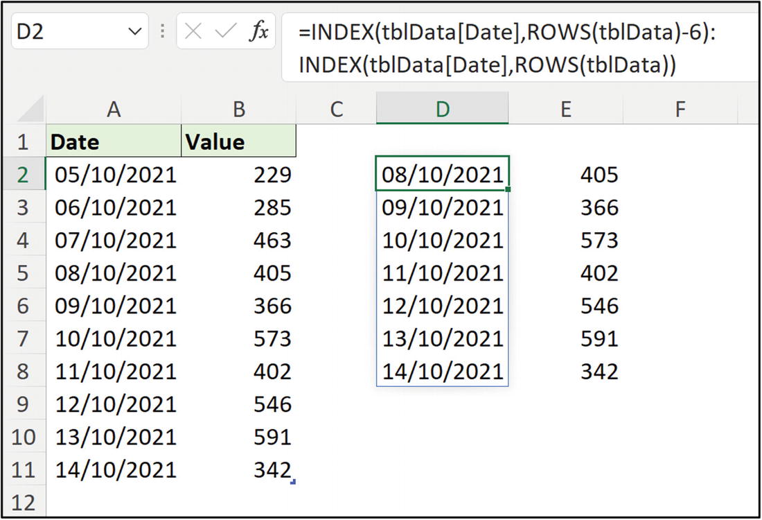
Moving Average Formula
This technique to return a range can be used to create calculations on dynamic ranges. A common example of this is the moving average calculation.
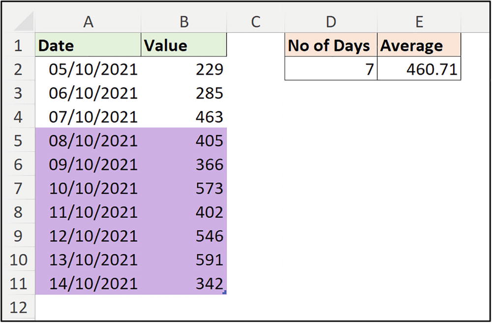
In this example, we have a table of values named [tblDaily], and we will use a moving average formula to return the average for the last seven days only.

Moving average formula using INDEX
The OFFSET function can also be used to create dynamic ranges. In fact, it is often a simpler approach. However, I prefer the INDEX function.
Working with Arrays and Spilled Ranges
The INDEX function is fantastic for working with arrays. It enables us to extract specific rows, columns, or cells from arrays and from the spilled ranges of other formulas. Let’s see some examples.
Creating a Top N List
A great example of the INDEX function extracting specific rows from an array is when used with SORT to create a top N report.
Figure 11-73 shows a table named [tblProductSales]. It is a small table for the purposes of this demonstration.

Table of product sales
Two SEQUENCE functions are then used – one to return the rows and another for the columns.
The first SEQUENCE function uses the value stated in cell C2 for the number of rows to return. If the value is 5, the SEQUENCE function returns an array of {1, 2, 3, 4, 5}. So, the first five rows are returned. The number of rows is dependent on the value in cell C2.

Top N report with INDEX, SORT, and SEQUENCE
Extracting Headers from a Table/Range
Functions such as SORT, FILTER, and many others do not return headers with a returned array, especially when based on a data formatted as a table. This is a good thing, because headers are not data and therefore should be kept distinct.
This means that the headers are typed or pasted into cells when creating a report in Excel. This is not much of an issue and indeed has its benefits (we will create dynamic headers shortly). However, if you want to return the headers using a formula, then this is simple. And when we require specific headers, then INDEX is up to the task.

Returning the header names with a simple formula
The rank column is not part of the original table data, so this header needs to be entered manually.
Returning Rows/Columns from a Spill Range
Extracting specific rows and/or columns from a spill range is no different to extracting them from a table or array.
For this example, let’s imagine we want to sum the total values from the spill range of the previous formula. This formula returned a spill range that is four columns wide. The [Total] column is the fourth column of the spill range. So, we need to specify that the SUM function uses column 4 only.

Summing a specific column from a spill range
Instead of entering the index value of 4 for the col num, sometimes using a function may be a better option, as it is dynamic. We will see examples of dynamically returning columns in the next example.
Returning Non-adjacent Columns from a Table with INDEX-MATCH
Functions such as FILTER, SORT, and SORTBY do not natively allow the selection of specific columns from a table or array. They will only allow the return of a group of adjacent columns. Fortunately, we know INDEX, and INDEX does not understand the words “it can’t be done.”
The INDEX and MATCH/XMATCH combination provides an effective way to dynamically return specific columns from a table or array using cell values.

Returning specific columns from an array with INDEX-MATCH
The CHOOSECOLS function is covered shortly and is a great alternative method for returning specific columns from an array. CHOOSE has also been discussed in this book. It is fantastic to have so many different options for this task.
In this example, INDEX was already being used to return the top N values, so was the obvious choice in preference of the aforementioned functions.
Returning a Reference from a List
In this final example of the INDEX function, we will be using its second syntax. By using INDEX in this way, we can internally list a collection of references, and then return the reference we want dynamically using an index number.
For this example, we will be using the table of sales data shown in Figure 11-78. This shows only the first few rows of the table named [tblData].
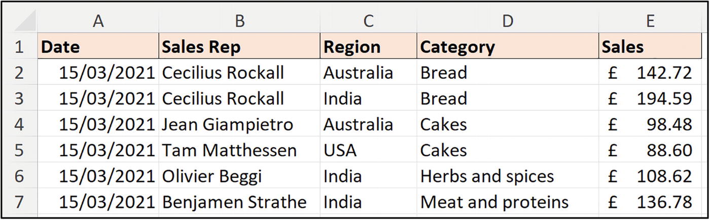
Table of sales data
In Figure 11-79, the drop-down list with the three column names is in cell C2, with “Region” currently specified.
The first argument within INDEX is the collection of references. The three columns [Category], [Region], and [Sales Rep] are entered here within brackets. The order is important, as they are indexed as references 1, 2, and 3.
The row num and column num arguments are ignored as we want to return all values for the stated column.
The MATCH function is entered in the area num argument. It searches for the value stated in cell C2 within the range A1:A3 and returns the index number of the found value. It is essential that the order of the references in range A1:A3 match the order of the references in the first argument of INDEX.

Using INDEX to dynamically return row labels
This is a pretty cool technique that further demonstrates the sheer number of tasks that INDEX can help us to achieve. However, this type of task is easier to accomplish with the CHOOSE or INDIRECT functions or by using a newer function such as SWITCH or XLOOKUP.
CHOOSECOLS and CHOOSEROWS Functions
Availability: Excel for Microsoft 365, Excel for the Web, Excel for Microsoft 365 for Mac
choosecols-and-chooserows.xlsx
The CHOOSECOLS and CHOOSEROWS functions are very new functions that have been released to Excel 365 and Excel Online only, during the writing of this chapter.
They have been introduced to simplify the extraction and ordering of specific columns or rows from a table or array.
There have been examples in this book that use functions such as CHOOSE and INDEX to perform these tasks. And they are great, especially CHOOSE as it offers a specific advantage over these new functions. That advantage is that you can specify columns absolutely. This is very helpful, especially when data is formatted as a table.
However, these are the new kids in town, and they are fantastic. The columns or rows you require are specified by providing the column or row index numbers. The true power of these functions is realized when functions such as SEQUENCE, COUNTA, and MATCH are used to return the column or row numbers.
Array: The table, range, or array that you want to return specific columns of rows from.
Col num or Row num: The index numbers for the columns or rows that you want to return from the array. The column and row numbers can be entered as separate arguments or provided as an array of index numbers.
CHOOSECOLS to Return Specific Columns
The CHOOSECOLS function, as its name beautifully describes, enables us to choose specific columns from an array. This function has been eagerly awaited by Excel users as soon as we realized that dynamic array functions such as SORT and FILTER would not allow the selection of non-adjacent columns.
Now, we know that there are already preexisting methods of overcoming this issue such as the INDEX function. But the CHOOSECOLS function is built for this purpose and is therefore simpler and more discoverable by Excel users needing this functionality.

Table of product sales data

CHOOSECOLS returning the first and fourth columns only
CHOOSECOLS with MATCH
Typing the column index numbers to be returned is not ideal, especially with tables that have many columns. The MATCH function can be used to return the column numbers based on cell values.
Because of this functionality, other functions can be used to return the array of column numbers to CHOOSECOLS.
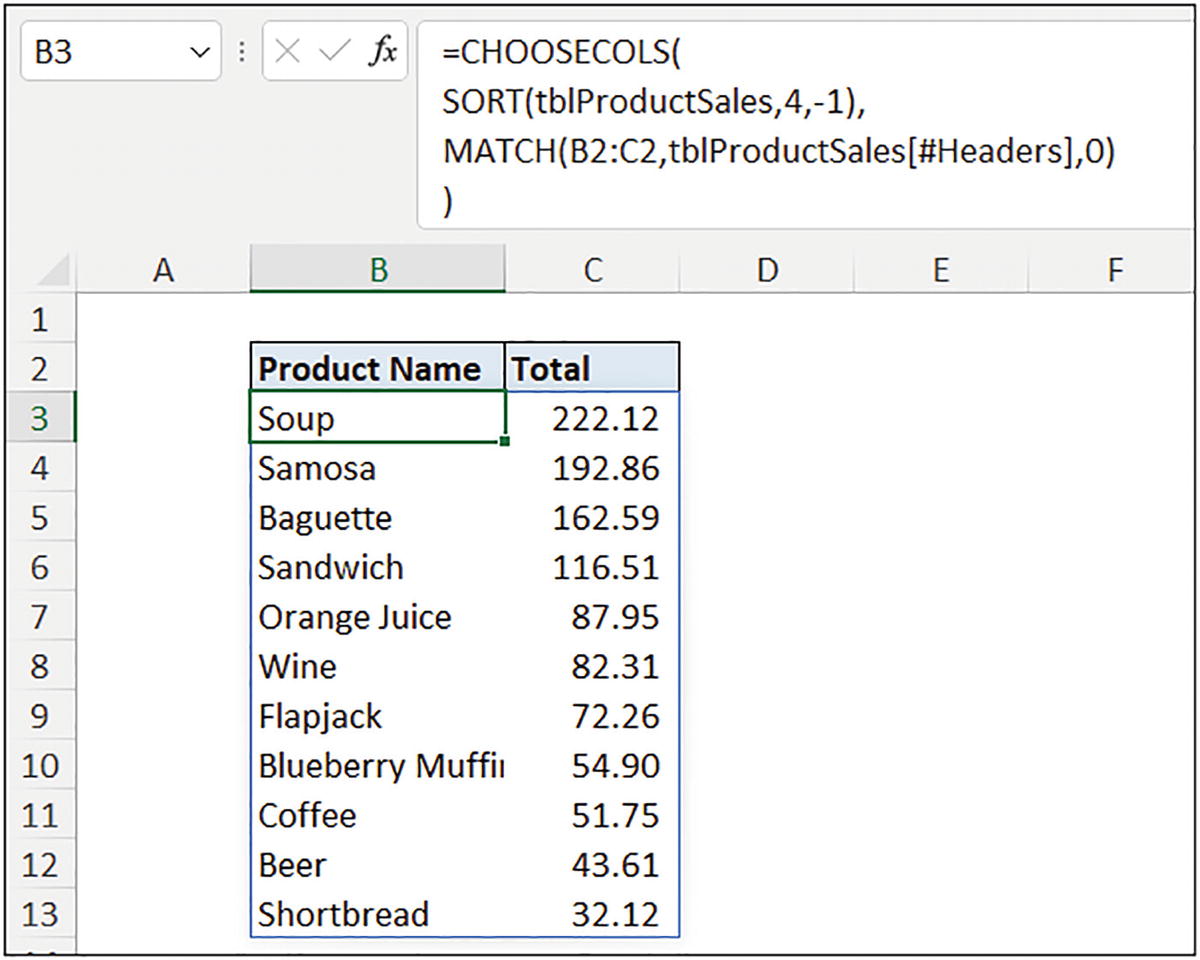
CHOOSECOLS with MATCH for dynamic column numbers
This technique does require that the values in range B2:C2 match the header name exactly. However, it also means that you can change the value in cell B2 or C2 to return a different column, for example, “Product Name” to “Category.” This could be a cool feature in a reporting scenario.
CHOOSE for Absolute Column Selection
I know, I know, the CHOOSE function has been covered in this chapter and in other parts of this book already. But it feels appropriate to demonstrate it here along with CHOOSECOLS as an alternative approach.
CHOOSECOLS is great for dynamic reports and models. It can be combined with other formulas or controls to return the column numbers such as MATCH and SEQUENCE. But you may want to just specify the columns to return by their name. And in that scenario, one could argue that CHOOSE is better.

CHOOSE and SORTBY alternative formula
The structure of this formula is different to before in respect that CHOOSE is serving an array to SORTBY, while previously SORT was serving CHOOSECOLS with the array. So, the sequence is reversed.
In simple examples, you can choose the method that you prefer. CHOOSECOLS offers more potential when it comes to dynamic, robust, and interactive spreadsheets.
Finally, with the CHOOSE example, if there were many columns to return, the SEQUENCE function could be added to avoid entering the sequence of column numbers manually.
Reordering Columns with CHOOSECOLS
In addition to returning specific columns from an array, CHOOSECOLS enables us to position the columns in any order that we require.
Following on from the previous examples, let’s return the [Category], [Product Name], and [Total] columns from the SORT function and position them in the order just stated.

Order of columns in the product sales table

CHOOSECOLS changing an array’s column order
In this example, the MATCH function could have been used to return the column numbers from range B2:D2 instead of the entry of the 2, 1, 4 numbers, if preferred.
Returning Every Nth Column
By combining the CHOOSECOLS function with SEQUENCE, you can return all columns that occur at specific intervals.

Table of quarterly data
In this example, the columns that we require occur in every fourth column. We want to return columns 1, 5, 9, 13, and 17.
In the SEQUENCE function, the number of columns to return is calculated by dividing the total number of table columns by 4 and rounding the result up. In this example, this results in 17 divided by 4 equals 4.25. This is then rounded up to 5. So, 5 columns are returned. The step argument of SEQUENCE is entered as 4.
This approach can be used for any number of columns and any divisor that you require.

Returning every Nth column with CHOOSECOLS and SEQUENCE
CHOOSEROWS to Return Every Nth Row
The CHOOSEROWS function is used to return specific rows from an array. This function is generally not as commonly used as CHOOSECOLS, because there are many other Excel functions to return rows, and values from rows, including FILTER and VLOOKUP.
The FILTER function enables us to return rows from a table that meets specific criteria. So, the specific advantage of CHOOSEROWS is that we can specify the exact rows we need or the rows that follow a specific pattern.
In Figure 11-88, we have a table containing payments that have been received from different sources. The table is named [tblPayments], and it contains subtotal rows.

Table of payment data that includes subtotals

CHOOSEROWS function returning every third row
Returning the Top and Bottom N Values
Another example where the CHOOSEROWS function can be useful is to return the top and bottom N values from an array.

CHOOSEROWS returning top and bottom N rows
TAKE and DROP Functions
Availability: Excel for Microsoft 365, Excel for the Web, Excel for Microsoft 365 for Mac
take-and-drop.xlsx
TAKE: The TAKE function is used to return a specific number of consecutive rows or columns from the start or end of an array.
DROP: The DROP function removes a specific number of consecutive rows or columns from the start or end of an array.
Array: The array from which to take or drop rows or columns.
Rows: The number of consecutive rows to take or drop. A positive value will take or drop rows from the start of an array, and a negative value will take or drop rows from the end of an array.
[Columns]: The number of consecutive columns to take or drop. A positive value will take or drop columns from the start of an array, and a negative value will take or drop columns from the end of an array.
The following examples will be based on the product data shown in Figure 11-91. For some examples, the data is formatted as a table named [tblProducts], and in others it is a range on the [Data] sheet.
The TAKE and DROP functions do not accept arrays of row or column numbers like CHOOSEROWS and CHOOSECOLS can.

Product data for take and drop examples
In the formula, 1 is entered for the rows argument and –2 for columns to remove the two columns from the end of the array.

Dropping rows and columns from a range
With the TAKE and DROP functions, both the rows and columns arguments are optional. However, you must provide at least one of these arguments.

TAKE function returning the first two columns from a table
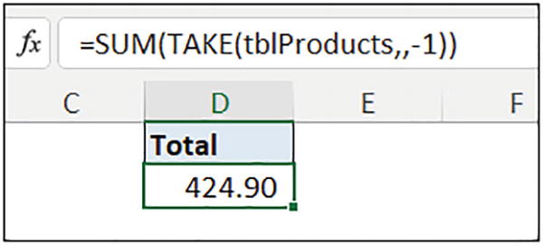
TAKE returning the last column only

The TAKE and DROP functions together in a formula
Finally, the TAKE and DROP functions can accept arrays from other functions and the number of rows or columns from a cell value.
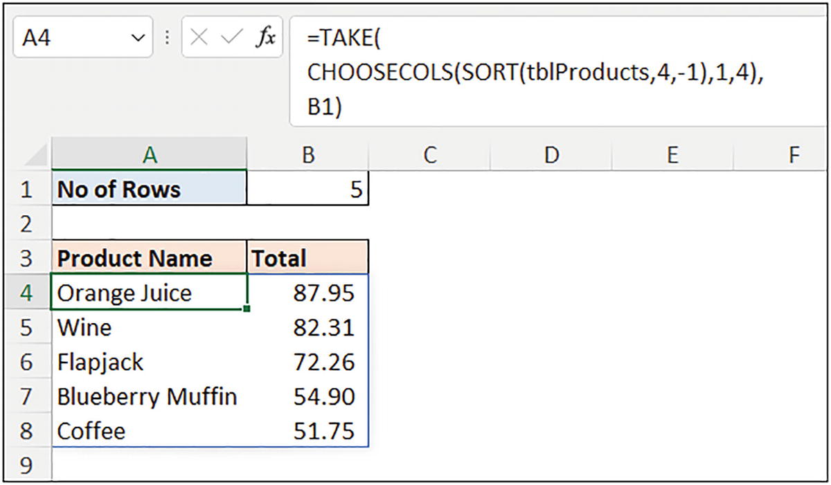
Using a cell value to specify the number of rows
VSTACK and HSTACK Functions
Availability: Excel for Microsoft 365, Excel for the Web, Excel for Microsoft 365 for Mac
vstack-and-hstack.xlsx
The VSTACK and HSTACK functions are used to combine, or stack, multiple arrays vertically or horizontally into a single array.
These functions have been eagerly anticipated by Excel users. They make particular tasks that were once awkward now very easy.
Array1, [array2]: The arrays that you want to stack vertically or horizontally
Stacking Multiple Tables with VSTACK
Combining multiple tables is a task that previously required endless copy and paste operations, a Power Query, or a macro to perform. Now, with VSTACK, it is incredibly simple and will automatically update when data in the tables update.

Multiple tables to be stacked

Stacking tables together into a single table
Adding Calculated Columns to an Array with HSTACK
The HSTACK function is used to stack arrays horizontally. This function can be great for adding calculated columns to an array. With the VSTACK and HSTACK functions, we can create reports with a single formula.
For an example of this, we will create a report that we have covered previously in this book, but this time, with a single formula.
The HSTACK function is used again in Chapter 15 to create our own function that generates a report.

Table of sales data
The HSTACK function combines two arrays together. The first array is the distinct list of product names. And the second is the SUMIFS function to return the total for each product name.
The SORT function then sorts the returned array by the second column in descending order.
The HSTACK function can handle more than two arrays, so more calculated columns can be added if required.

Creating a report with one formula
Lookup Functions with Other Excel Features
Lookup functions are some of the best functions to use with other Excel features. With functions such as INDEX, INDIRECT, and CHOOSEROWS, you can create some cool dynamic functionality to charts, Data Validation rules, and formatting in Excel.
Dynamic Data Validation List with INDEX or OFFSET
One of the most common requirements for the INDEX and OFFSET functions is to create a dynamic range. And a reason for this can be to feed a Data Validation list. When items are added or removed from the range used as the source for the list, the list automatically updates to include or exclude the items.
My personal preference for this task is to use the INDEX function, but it is useful to be familiar with both.
Figure 11-101 shows four separate ranges of city names by country. For each range, additional cities may be added, or some removed over time. We want to make these ranges dynamic to accommodate such changes automatically.

Different lists of cities by country
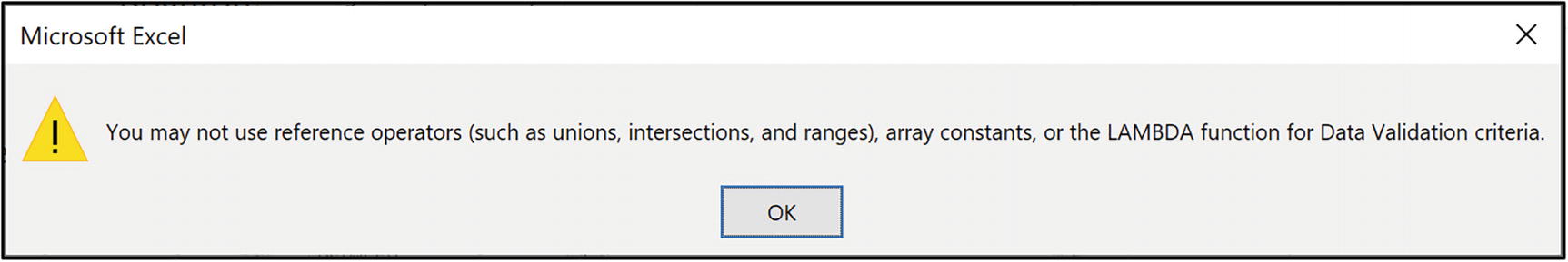
Error due to use of the range operator in a Data Validation rule
A name will need to be defined for the formula, and that name is then used in the Data Validation rule. Even if we were able to enter it directly, I would be inclined to define a name anyway for better management of the workbook.
Figure 11-103 shows the formula entered as the source for a name defined as “lstGermany.”

Define a name for the dynamic range
- 1.
Click Data ➤ Data Validation.
- 2.
On the Settings tab, select List for the Allow list and enter the following reference in the Source box (Figure 11-104). Click OK.

Data Validation list using lstGermany as its source
This formula can be entered directly into the Data Validation rule as it does not include a range operator or other illegal characters. This, I suppose, is an advantage over INDEX, though I do like the concept of defining names for ranges such as this still.
You may be thinking “if a Data Validation list is based on a range formatted as a table, would the list auto-expand and contract in size with the table?”. Well, at the time of writing this book, a Data Validation list only effectively updates with a table when they are on the same sheet.
Now, we do not need this formula approach, because if we simply define a name for a range formatted as a table, the name and table work together to create the dynamic range.
However, due to this confusion, until Microsoft has a Data Validation rule and table data working together efficiently, using INDEX or OFFSET for a dynamic range is still very beneficial. It should also be noted that understanding this technique assists us in scenarios outside of Data Validation list too.
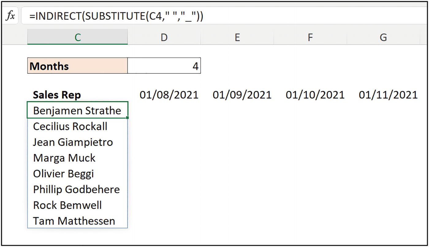
Dependent Data Validation List with INDIRECT
Creating dependent drop-down lists with Data Validation is a common question asked in training courses and across Excel forums. Often, a list of items is too large, and it is useful to have a first list that reduces the items shown in a second list.
In modern Excel versions, the searchable list functionality recently introduced has lessened the requirement for creating dependent drop-down lists. But this is only available for those using Excel 365 or Excel Online. This technique is still important for previous Excel versions.

Ranges of city names by country

Setup for dependent list
- 1.
Click cell D3.
- 2.
Click Data ➤ Data Validation.
- 3.
On the Settings tab, select List for the Allow list and enter the following INDIRECT formula in the Source box (Figure 11-107). Click OK.
This formula creates a reference by combining the text string “lst” with the value in cell B3. This allows us to indirectly reference the named range of cities for the country stated in cell B3.
This technique works for named ranges only, and not for named formulas.

INDIRECT for a dependent drop-down list

List of cities dependent upon country selection
Although this example shows the dependent drop-down list in a single cell, it can be applied to multiple cells. The reference type in the INDIRECT function would need modifying to fit the sheet layout, that is, $B3 for multiple rows.
In this example, all country names are single words – Germany, Spain, UK, and USA. If there was a country with more than one word in its name such as South Korea or New Zealand, then the formula would be a little different.
Why? Well, you cannot use spaces in the name of a range, yet the name of the range and the name of the country selected in cell B3 must match exactly.
A common solution for this is to use an underscore in the named range of that country’s cities, that is, lstnew_zealand. The name of the country in the first drop-down would be “New Zealand,” as one would expect.
Format Last X Number of Rows
In the INDEX function part of this chapter, we saw INDEX used to calculate the moving average for a specified number of days. Now, this could be any calculation; the key is that the range being calculated is moving as new rows are added to a table.
For a nice visual touch, it has been decided to format the rows being used in the calculation.
We will use the OFFSET in a Conditional Formatting rule for this task. INDEX would be an obvious choice for this task, but mixing up the techniques used is good for learning.
Format the last x number of rows
- 1.
Select the table.
- 2.
Click Home ➤ Conditional Formatting ➤ New Rule.
- 3.
Click Use a formula to determine which cells to format.
- 4.
Enter the following formula into the Format values where this formula is true box (Figure 11-110):
- 5.
Click Format and specify the format to apply. Click OK.
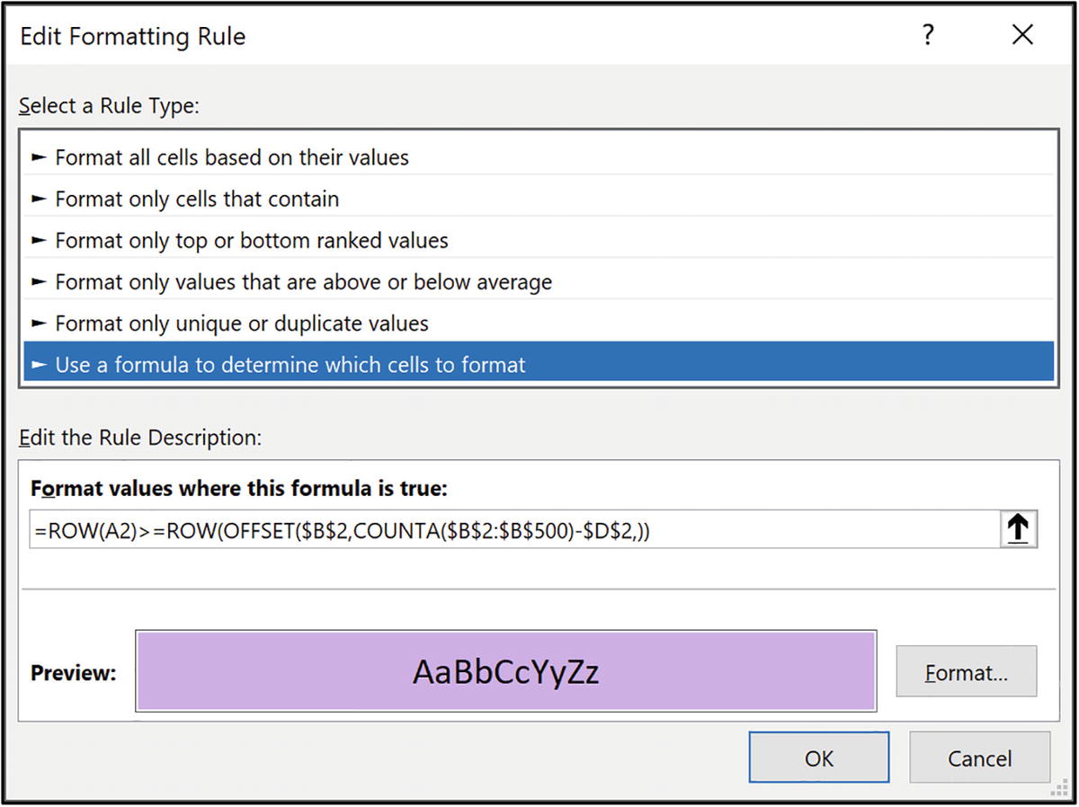
Conditional Formatting rule to format the last x number of rows
Interactive Chart with INDIRECT
The INDIRECT function offers a simple method to return data from a table dependent upon user selection. In this example, we have four tables containing sales data (Figure 11-111). Each table shares its name with the name of the city written above the table prefixed by the characters “tbl”.
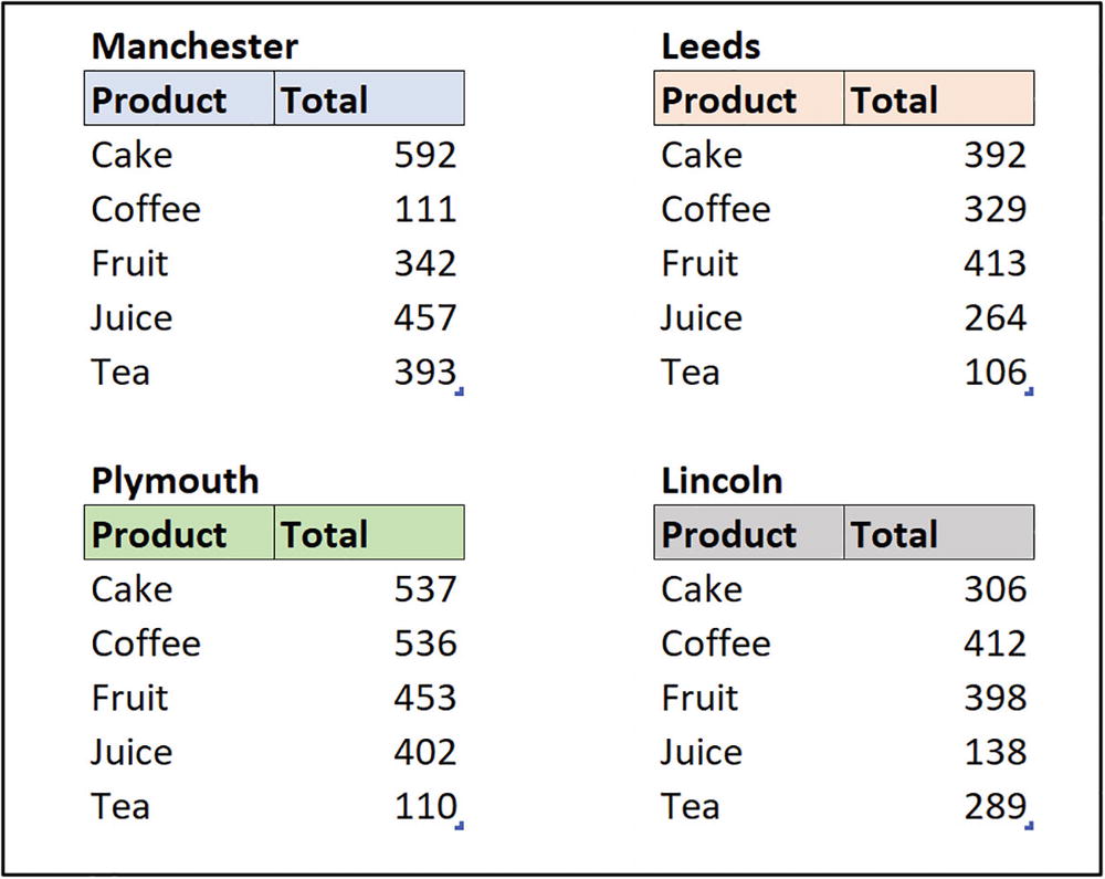
Four sales tables to be used for the chart source

INDIRECT function returning data dependent upon cell value
The INDEX function is wrapped around the INDIRECT function to return the value from the row and column numbers of cell A1. So, the formula in cell B5 returns the value from row 1 and column 1 of the [tblLincoln] table.
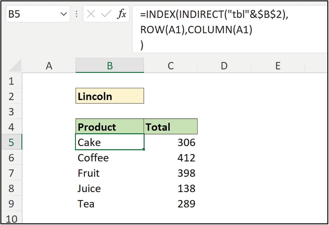
INDIRECT with INDEX for a non-dynamic array method
- 1.
Select range B4:C9.
- 2.
Click Insert ➤ Insert Column or Bar Chart ➤ Clustered Column.

Column chart presenting data from the tblLincoln table
Interactive Chart with CHOOSEROWS

Table of monthly data
We want to chart all monthly values for the name selected from the drop-down list in cell C2 (Figure 11-116). This cell has been named [rngName].
The row of values that we require is specified by a cell value, so a combination of CHOOSEROWS and MATCH would be a nice choice of functions for this task.

Drop-down list of names for interactive chart

CHOOSEROWS formula entered on the sheet

Using INDEX and SEQUENCE as an alternative to CHOOSEROWS and DROP
The formulas have been entered on the sheet to check the results and that they function correctly before proceeding with the chart.
- 1.
Click Formulas ➤ Define Name.
- 2.
In the New Name window, type a Name for the chart values. Then click in the Refers to box, and click cell A2 that contains the formula on the sheet [CHOOSEROWS Data]. Add the “#” on the end to reference the dynamic spill range. In Figure 11-119, the reference has been named “chooserowsValues”. Click OK.

Defining a name for the CHOOSEROWS formula
- 3.
Repeat these steps for the formula that returns the chart labels. In this example, this formula has been named “chooserowsLabels”.
- 4.
Click Insert ➤ Insert Line or Area Chart ➤ Line.
- 5.
Click Chart Design ➤ Select Data.
- 6.
In the Select Data Source window, click the Add button in the Legend Entries (Series) area of the window.
- 7.
In the Edit Series window (Figure 11-120), click in the Series values box, remove any text, click a cell on the sheet to enter a sheet name, remove the cell reference, and type “chooserowsValues”. Click OK.

Adding the defined name for the series data of the line chart
- 8.
Click the Edit button in the Horizontal (Category) Axis Labels part of the window.
- 9.
In the Axis Labels window, click the Axis label range box, click a cell on the sheet, remove the cell reference, and type the name used for the labels “chooserowsLabels”. Click OK.
- 10.
Click OK to close the Select Data Source window.

Line chart plotting the values for Janet
Rolling Chart with INDEX
For the final example, we will create a rolling chart using INDEX to chart the last seven days of values. With INDEX, we can create a dynamic range easily. This makes it perfect for the task of creating a chart that presents the last x number of values only, that is, the last 13 months, the last 6 weeks, etc.
This technique was demonstrated earlier in the chapter to create a moving average formula with INDEX. This time, we will chart the values instead of aggregating them. When new rows are added, the chart automatically adjusts.
Figure 11-122 shows the results of these formulas being returned to the sheet. This is only done to help write them and to test their functionality.
Rolling data ranges using INDEX
- 1.
Copy the formula that returns the dates in cell D2. This name will form the axis labels of a line chart.
- 2.
Click Formulas ➤ Define Name.
- 3.
In the New Name window, type a Name for the date labels. Click the Refers to box and paste in the formula. In Figure 11-123, the formula has been named “dateLabels”. Click OK.

Defined name for the date labels
- 4.
Repeat these steps for the formula that returns the chart values. In this example, this formula has been named “chartValues”.
- 5.
Click Insert ➤ Insert Line or Area Chart ➤ Line.
- 6.
Click Chart Design ➤ Select Data.
- 7.
In the Select Data Source window, click the Add button in the Legend Entries (Series) area of the window.
- 8.
In the Edit Series window (Figure 11-124), click the Series values box, remove any text, click a cell on the sheet to enter a sheet name, remove the cell reference, and type “chartValues”. Click OK.

Adding the chartValues name for the chart data series
- 9.
Click the Edit button in the Horizontal (Category) Axis Labels part of the window.
- 10.
In the Axis Labels window, click the Axis label range box, click a cell on the sheet, remove the cell reference, and type the name used for the labels “dateLabels”. Click OK.
- 11.
Click OK to close the Select Data Source window.

Line chart showing the last seven days’ values only
Summary
In this chapter, we learned many of the best lookup functions in Excel, including INDEX, OFFSET, MATCH, and INDIRECT, to name a few. We also covered functions newly released to 2022, including VSTACK, CHOOSECOLS, and DROP. Excel is forever expanding and evolving.
This was a large chapter containing many practical examples to demonstrate the application of the different functions.
In the next chapter, we will focus on the XLOOKUP function in Excel, another lookup function. XLOOKUP deserves a chapter to itself. It is an accomplished function with many key strengths over similar functions including VLOOKUP, HLOOKUP, and the INDEX-MATCH combination.