
When working with structured data in Excel, it should be formatted as a table. Tables are a feature in Excel that make managing and analyzing a group of related data much easier. A range of cells can be converted into a table at the click of a button.
Working with tables vs. cell ranges is to compare today’s smartphone to a rotary dial telephone. The difference in the accessibility of the data, automation, and simplicity of use is remarkable. In fact, there are features in Excel such as Slicers and Power Query that require a range to be converted to a table.
Now, this does not mean that every range should be formatted as a table. There are dynamic arrays (covered in Chapter 10), which are their own thing. And single cell inputs for your models and reports. But when working with data structured as a list, there are many benefits from having it formatted as a table.
This chapter will focus on how tables improve how we write and work with formulas. We will not discuss the numerous other benefits of using tables including formatting, PivotTables, Power Query, and the data model.
In this chapter, we begin by explaining the many benefits of using tables. We then look at how to convert a range to a table and some best practice for using them.
Finally, we will see the correct and best ways to access data in a table when using formulas. It is outrageously fast and simple.
tables.xlsx
Why Use Tables?
Meaningful references
Tables provide a simple way to reference a range of cells. Compare a formula that references tblLondonSales vs. London!$A$1:$G$1022. The table reference is much easier to read and write than the worksheet reference.
Super easy referencing in formulas
The ease at which you can access the different elements of a table is remarkable.
You can select the elements of a table in a similar way that you would select a range of cells, or you can type the reference.

Referencing table elements from a formula
Tables are dynamic.
When additional rows or columns are added to a table, it automatically expands. Therefore, any formulas that reference that table will use the updated range.
When using a range of cells on the grid such as A2:D10, you cannot be sure that your formulas are using the correct range when you or your colleagues add and remove data from that range. It is less reliable and more awkward to update, especially if many formulas are using that range.
Users will commonly use tricks such as referencing entire columns in a formula, such as, $E:$E, or inserting rows into the middle of a table instead of at the bottom. These tricks help to ensure that any rows added to the range are included in the formulas.
Additional functionality
Tables enable additional functionality that is not in the scope of this book. This extra functionality includes the power tools such as Power Query and Power Pivot, using Slicers and consistent formatting.
Format a Range As a Table
So, tables are fantastic. Let’s look at how to convert a range into a table and then cover some essentials and best practices.
Creating a Table
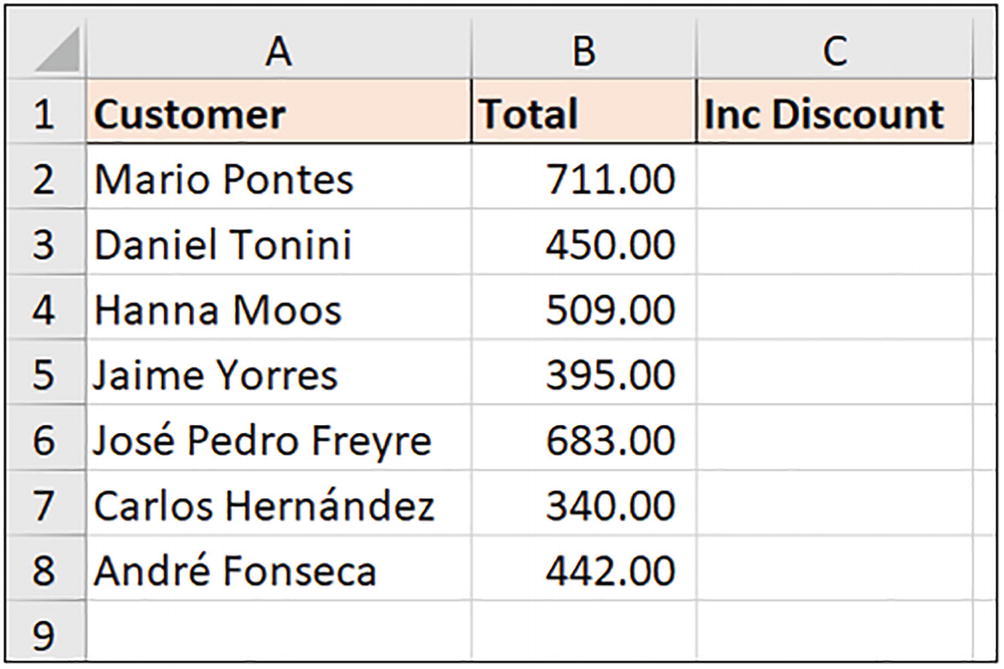
Range of data that needs converting to a table
- 1.
Click a cell within the range.
- 2.
Click Insert ➤ Table or press Ctrl + T.
Note You can also click Home ➤ Format as Table and click a style from the list.
- 3.
In the Create Table window (Figure 4-3), check that the range is correct and that the My table has headers box is checked (there are headers in the first row of the range). Click OK.
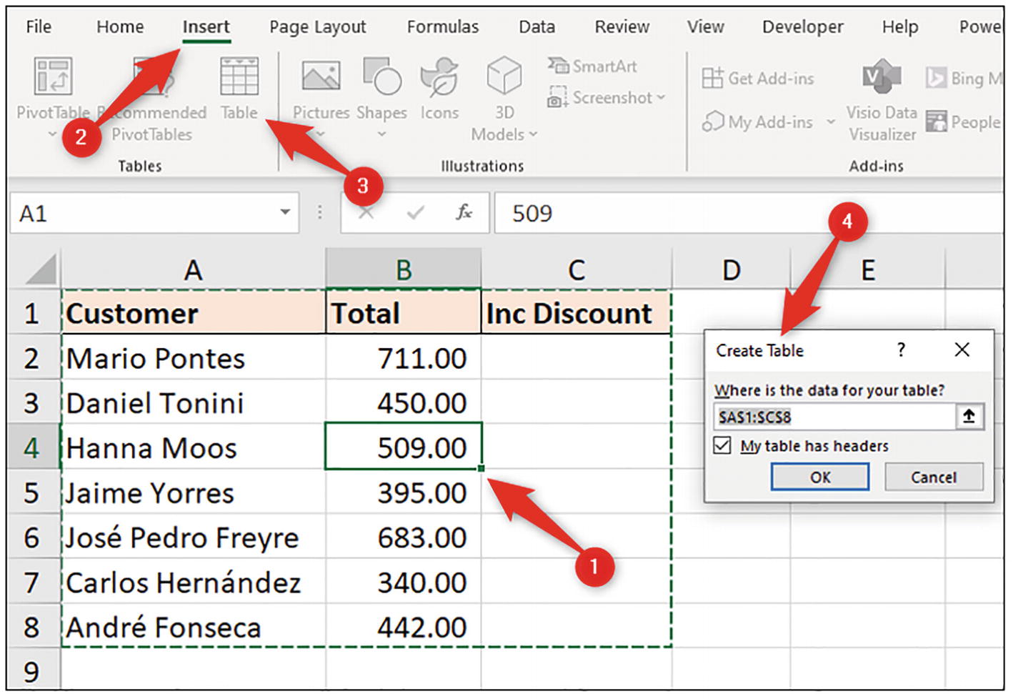
Create a table from a range
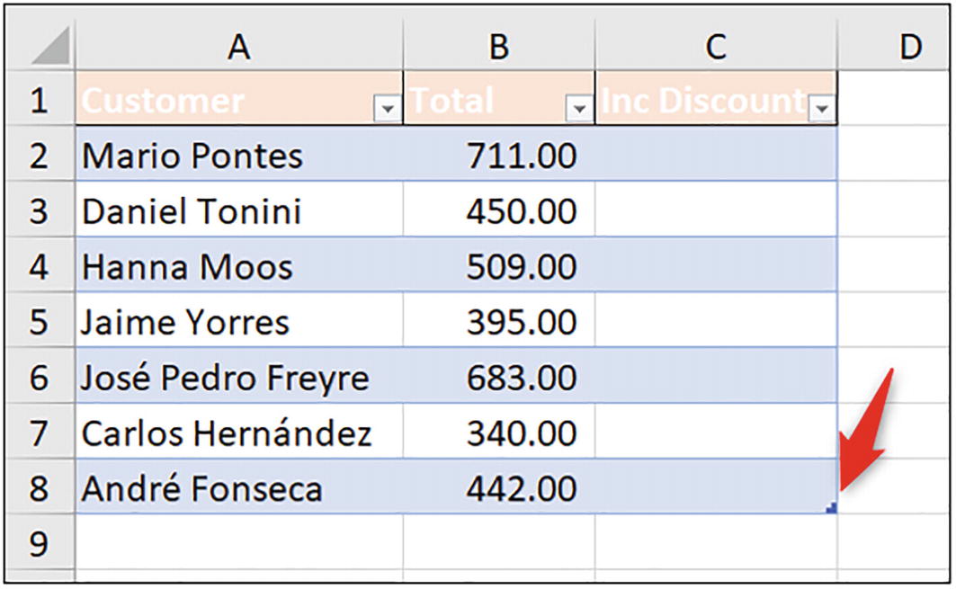
Table with the default style
The default style is applied. This style keeps any existing formatting that was applied to the range, such as the orange fill color in the header row.
It applies the elements of the default table style to areas where no previous formatting was specified. This includes the blue banded rows, blue border, and white font in the header row.
In the bottom-right corner of the table is a blue resize handle (Figure 4-4). This identifies the last cell of a table and can be used to quickly resize it if necessary.
Changing or Removing Table Styles
You can easily change or remove the table style if you are not contented with the default style applied. You can even create your own styles, but we will not be looking at this in the book.
- 1.
Click a cell within the table.
- 2.
Click Table Design and then the More button in the corner of the Styles gallery (Figure 4-5).
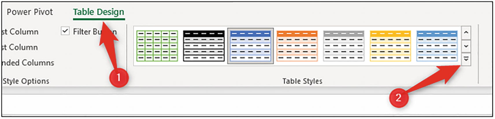
More button of the Styles gallery
- 3.
The gallery expands. You can choose a different style, create your own, or clear the style. To clear a style, click Clear at the bottom of the gallery, or click the None option (Figure 4-6).

Clear the table style

Table with no style applied
You can see the blue resize handle in the bottom-right corner. Also, the Table Design tab appears when the table is active. These are two signs that the range is formatted as a table.
Naming the Table
- 1.
Click a cell within the table.
- 2.
Click Table Design and enter the name you want to use in the Table Name box (Figure 4-8). In this example, it has been named “tblCustomerSales”.

Naming a table
The tbl prefix has been used to denote a table. This is optional but is a useful tip to easily distinguish tables from other names.
Working with Tables
When working with a workbook that contains tables, you may need to find, view, and edit these tables at some point.

Viewing tables in the Name Manager
To open the Name Manager , click Formulas ➤ Name Manager.
From the Name Manager , you can view all tables and see what they refer to.

Using the Name Box to navigate to a table

Using the Go To window to navigate to a table
These same methods can be used to navigate to named ranges and were covered in the previous chapter.
Table References in a Formula
This is an Excel formulas book, so we have now arrived at the exciting part. How do we reference the table and its elements from within a formula?
The Magic of @
Let’s begin by using a formula that references a single cell of the table. We will use the [tblCustomerSales] table that was just created.

IF function that references cells in the Total column
When clicking cell B2 while writing the formula, it is referenced as [@Total]. Total is the name of the column, the @ symbol refers to the same row within the table, and it is all enclosed in square brackets.
The names [rngThreshold] and [rngDiscount] refer to cells F2 and F4, respectively.
This is a very meaningful reference. Using the column header [Total] has greater meaning than column B.
And what is extra cool is that every cell in the [Inc Discount] column (column C) contains the same formula. If we used a range, the formulas would all be a little different as they would reference B3, B4, B5, and so on.
Another awesome feature when writing formulas that refer to a single cell on the same row in a table is that they automatically fill down to the last row. No need to click and drag or double-click that fill handle.
If you reference a single cell in a table on a different row to the active cell, then a grid reference is used. So, if you clicked on cell B3 while writing a formula in cell C2, then the reference to B3 is used. This is because there is no obvious relationship between two different rows of a table (rows 2 and 3 in this case) that Excel can recognize.
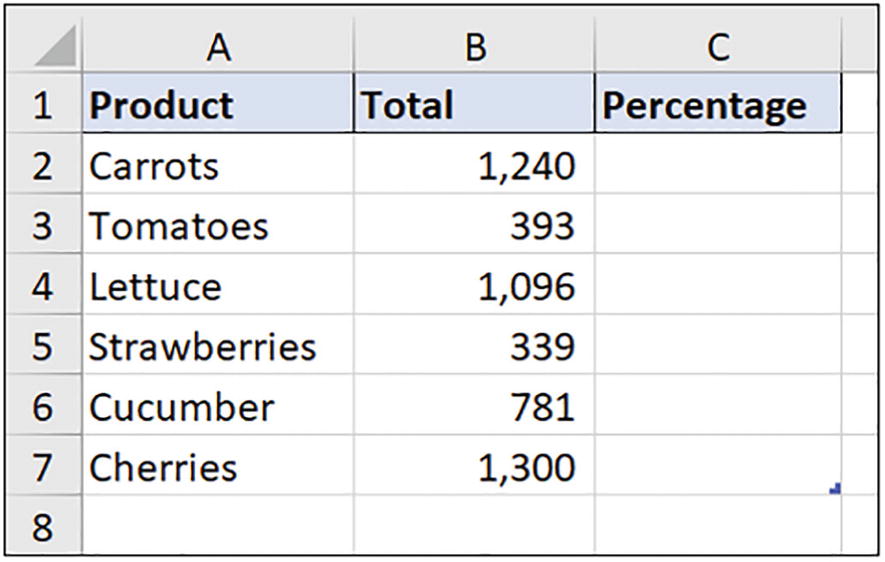
tblProducts showing product sales
We will write a formula in the [Percentage] column that calculates the percentage contribution that the sales of each product have made to the grand total.
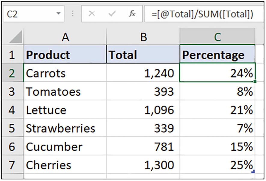
Percentage of column total
This formula includes a reference to a single product total, shown as [@Total], and a reference to the column, shown as [Total] (without the @ sign).
I think this is a good example of the use of the magic @ sign and how readable these formulas are when referencing table data.
When I read the @ symbol in my head, I like to say the word “this.” So, the formula reads “this total divided by the sum of totals” to me.
The cells where the formula is input are formatted as a percentage. However, Excel appears to change the cell formatting when this formula is entered. So, you may be required to format the [Percentage] column as percentages again.
Referencing Table Elements
A table is made up of a few elements. These include the header row, total row, the columns, the data minus the headers, and everything (data and headers). We will see examples of referencing these different elements as we progress through the book.
You can reference these table elements by selecting or clicking with your mouse or by typing the reference directly into the formula. I am a big fan of typing table references. It is so fast and easy. Let’s look at both methods.
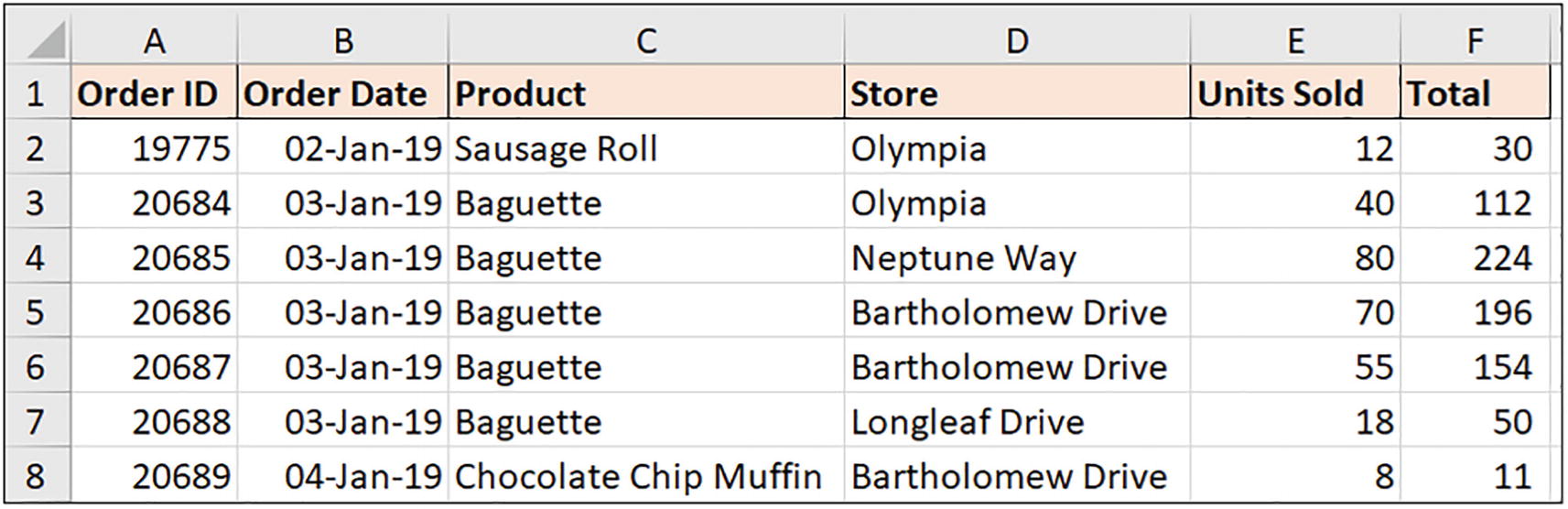
tblSales containing a list of orders
On the [Report] worksheet, we will use the SUMIFS function (covered in Chapter 8) to sum the [Total] column for the sales of a specific product.

SUMIFS function summing sales of coffee only
The name of the table precedes the column name as we are referencing the column from outside of the table.
To reference the columns, you can click the column header. This is great, but you must be careful.

Clicking a table column

Clicking a sheet column
The sheet column header changes to a green fill to illustrate this. However, this is easy to miss during the excitement of writing formulas.
You can also select the header row of a table and the entire table in a similar way. Be careful not to select the sheet row or column by mistake.

List of table elements as you type a formula
The list appears when the opening square bracket is typed.
Make Table Column and Cell References Absolute
Single column table references such as [@Product] and [Product] are relative by default, just like references to cells on a worksheet such as B2. Unfortunately, it is a little more awkward to make table references absolute.

SUMIFS function with table references
This works great!

All table column references have shifted to the right
All three table column references have changed.

The columns of tblSales
Now, there are a few ways to prevent this behavior.
One method is to copy or fill the formula using an alternative method to the classic drag of the fill handle.
You can click in cell G3 and press Ctrl + R to fill the formula right; the table references do not change. This is a terrific alternative.
Or you can copy the formula from the Formula Bar of cell F3 and paste it in cell G3. The table references do not change using this method either.
Finally, we could make the references absolute. To do this, you change the reference to a range and add an extra set of square brackets.

Absolute table references in a formula
Fixing the table columns in the formula is a more reliable method. It provides protection against other users of the sheet who may copy the formula.
However, the formula is more awkward to read, so it is useful to know the alternative methods such as Ctrl + R. Different situations can warrant a different approach.
Tables with Other Excel Features
Throughout this book, we will see examples of using formulas with other Excel features such as charts. If we are entering formulas within tables, it is important to understand how other Excel features work with tables.
Dynamic Lists
In the previous chapter, there was an example of creating a dynamic name using a formula. This name was then used as the source of a Data Validation list.
Tables are dynamic, so offer a wonderful alternative to this approach. Now, unfortunately tables do not work directly with Data Validation. You cannot enter a formula that uses the structured references of a table within a Data Validation rule directly. So, we will create a defined name for the table data and then use the name for the Data Validation list.

List of products formatted as a table named tblProductList
- 1.
Select the data range of the table, A2:A21.
- 2.
Click Formulas ➤ Define Name.
- 3.
Type “lstProducts” for the Name (Figure 4-25). Notice the table reference in the Refers to field.

Define a name for the list of products
We can then use this name for the source of the Data Validation list. Because the name understands the table, it works as a translator between the table and Data Validation features of Excel.
- 1.
Click cell B3.
- 2.
Click Data ➤ Data Validation.
- 3.
From the Settings tab, click the Allow list and select List.
- 4.
Type “=lstProducts” in the Source field and click OK (Figure 4-26).

Data Validation list using the defined name as its source
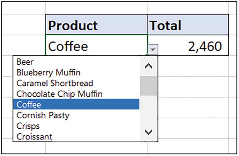
If more products are added to [tblProductList], they are automatically included in the Data Validation list.
There have been some major improvements made to Data Validation in recent months. So, at the time of writing this book, although we cannot directly use a Data Validation list from table data on another sheet, it may be a functional feature in modern Excel versions soon.
Such advancements will only be available to Excel for Microsoft 365 (Windows and Mac) and Excel for the Web, meaning this technique of using defined names is still very applicable.
Defined names have always had this special power to get two different Excel features working together.
Dynamic Charts
Using tables as the source of charts is a simple way to make your charts automatically update when new data is added to the table.

Line chart using table data
The table is in range A1:B6, and you can see that range highlighted when the chart is selected, showing that they are connected.
If we look at the chart data though, it does not reference the table that it is connected to.
Select the chart and click Chart Design ➤ Select Data.

Chart range is shown as a cell range despite using the table
Although it does not directly mention [tblMonthlySales], it is connected to it. This is a little confusing, but you get used to it.

Chart updates automatically when data is added to the table
Tables are an incredible feature of Excel, and many of the formula examples in this book will be using table references.
Summary
In this chapter, we learned how tables help us to manage and analyze structured data in Excel. We also learned how to effectively reference table data within formulas.
In the next chapter, we will learn the text functions in Excel. These functions enable us to split, extract, join, and format text. They are very useful, and we have many to discuss, so let’s start.