
6
Finite Element Method
6.1 Introduction
Finite element method (FEM) has wide applications in various science and engineering fields viz. structural mechanics, biomechanics and electromagnetic field problems, etc. of which exact solutions may not be determined. The FEM serves as a numerical discretization approach that converts differential equations into algebraic equations. In this regard, the weighted residual methods discussed in Chapter 3 convert governing differential equation to a system of algebraic equations over the entire domain Ω, whereas FEM is applied to finitely discretized elements of the global domain Ω. Also, the finite difference technique discussed in Chapter 5 generally considers the spacing of nodes such that the entire domain is partitioned in terms of squares and rectangles. The FEM overcomes this drawback as depicted in Figure 6.1 by spacing the nodes such that the entire domain is partitioned using any shape in general.
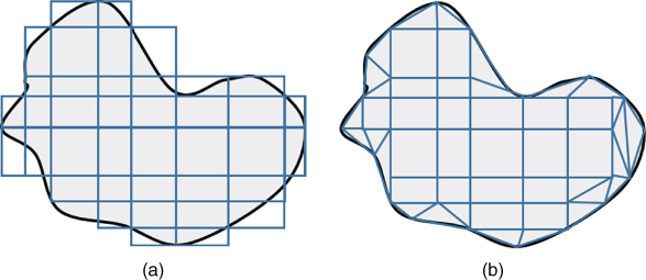
Figure 6.1 (a) Finite difference and (b) finite element discretization of arbitrary object.

Figure 6.2 Nodal points for the domain Ω = [a, b].
In this chapter simple differential equations are solved in order to have better understanding of the finite element technique. There exist various standard books [1–7] and the references mentioned therein devoted to the FEM and effective applications in various science and engineering fields. As such, this section gives an introduction to the FEM. Then, procedures of FEM and Galerkin FEM are discussed in Sections 6.2 and 6.3, respectively. Finally, the last section implements FEM for solving one‐dimensional structural problems.
6.2 Finite Element Procedure
In the FEM, the global domain Ω is partitioned finitely to a number of nonoverlapping subdomains known as finite elements. Generally, a two‐dimensional (2D) domain is partitioned in terms of 2D geometrical regions viz. triangles and quadrilaterals whereas a three‐dimensional (3D) domain is partitioned using 3D regions such as cuboids, tetrahedrons, pyramids, etc. Finite element partition of complex structural systems using different shape elements may be found in Refs. [8–10]. In this regard, the procedures involved in the FEM [8] are formulated as below:
- Divide the global domain Ω = [a, b] into finitely n subdomains or elements (Figure 6.2) as
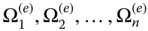 such that
 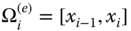 for i = 1, 2, …, n. Recall that xi are referred to as n + 1 nodes or nodal points where xi are not necessarily to be evenly spaced (Δxi = xi − xi − 1 is not same for i = 1, 2, …, n).
 - The approximate solution
 for the differential equation,
(6.1)subject to boundary conditions u(a) = γa and u(b) = γb is expressed in terms of element interpolating polynomials
for the differential equation,
(6.1)subject to boundary conditions u(a) = γa and u(b) = γb is expressed in terms of element interpolating polynomials
 ,
(6.2)
,
(6.2)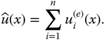
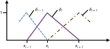
Figure 6.3 Shape function of Lagrange polynomial. - Consider the element interpolating functions
 as
(6.3)
as
(6.3)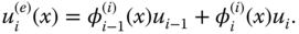
Here, φ are the interpolating functions that resemble the shape functions. For instance, the first‐degree Lagrange polynomial (given in Figure 6.3) for each element is
6.4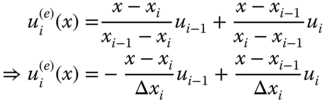
where the interval spacing is given by Δxi = xi − xi − 1.
Other interpolation polynomial approximations viz. Hermite [9, 10 ] may also be used.
- Obtain the system of equations known as element equations involving nodal values for each element that may be found using the Galerkin‐weighted residual method discussed in Chapter 3.
- Combine the set of element equations obtained using the Galerkin method. This method of combination is generally referred to as assembling. Apply the Galerkin‐weighted residual method to each element between the nodes xi − 1 and xi to obtain the nodal equations.
- Solve the assembled system of equations involving nodal points to obtain global approximate solution of governing differential equation for the entire domain.
For ease of understanding the FEM, the step‐by‐step procedure of linear second‐order ordinary differential equation (ODE) is considered with respect to the Galerkin method in Section 6.3.1.
6.3 Galerkin Finite Element Method
In this section, the steps [ 8 , 9 ] involved in solving differential equations 11,12] using the above‐mentioned procedure is discussed.
6.3.1 Ordinary Differential Equation
This section gives a detailed procedure for solving ODE subject to boundary conditions using the Galerkin FEM.
Let us consider a linear second‐order ODE,
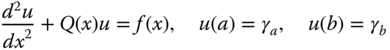
over the domain [a, b].
Step (i): Divide [a, b] into finitely n elements ![]() ,
, ![]() , …,
, …, ![]() such that x0, x1, …, xn are nodes.
such that x0, x1, …, xn are nodes.
Step (ii): Using Eq. (6.4), the element interpolating polynomial is considered as
having element shape functions
Step (iii): Apply the Galerkin method to each element i with respect to the weight function φk(x), where k = i − 1, i for obtaining element equations.
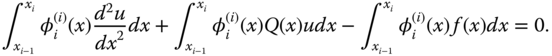
The weighted residual integrals I(u(x)) are obtained as

and

where ![]() is the residual. Equations (6.7a) and (6.7b) further get reduced to
is the residual. Equations (6.7a) and (6.7b) further get reduced to

and
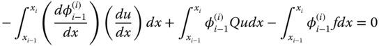
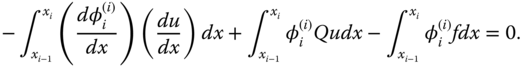
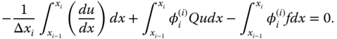
By applying integration by parts to Eqs. (6.8a) and (6.8b), we get
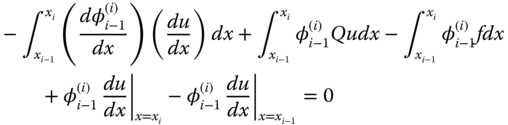
and
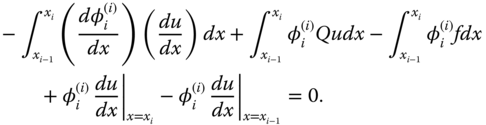
The shape function in the Galerkin method is selected such that ![]() is zero in all integrals except at ith integral and
is zero in all integrals except at ith integral and ![]() . As such, Eqs. (6.9a) and (6.9b) further reduce to
. As such, Eqs. (6.9a) and (6.9b) further reduce to
and
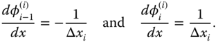
By using the shape functions given in Eq. (6.6), we have
By substituting Eq. (6.11) in Eqs. (6.10a) and (6.10b), one may obtain
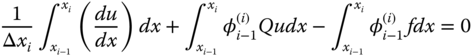
and
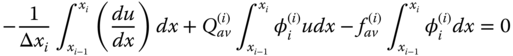
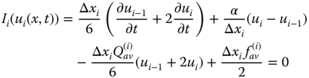
Taking average values for Q and f over the integral, Eqs. (6.12a) and (6.12b) reduce to
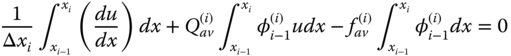
and
where ![]() and
and ![]() . Moreover,
. Moreover, ![]() , which yields
, which yields
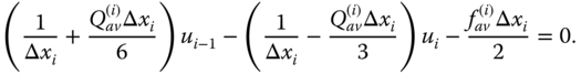
Equations (6.13a) and (6.13b) reduce to system of equations (element equations) for ith element,
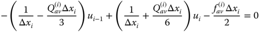
and
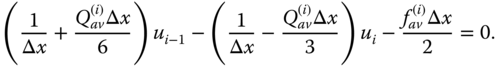
In case of equal spacing, the ith element system of equations gets transformed to

and
Step (iv): The element equations are then assembled to form a system of equations with unknowns u0, u1,…, un.
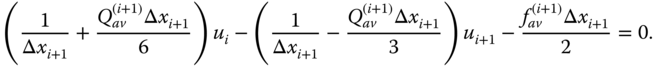
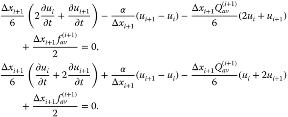
By using Eqs. (6.16a) and (6.16b), the element equations for (i + 1)th element is given by
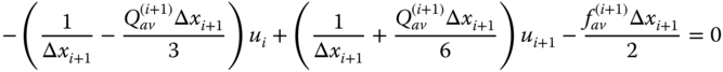
and
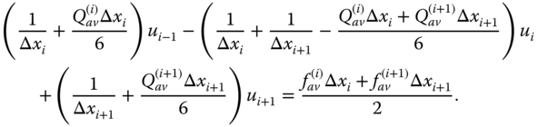
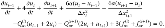
Hence, the nodal equation at (i + 1)th node is obtained by adding Eqs. (6.15b) and (6.17a),
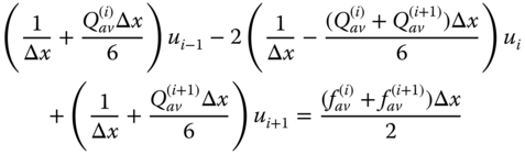
Then, Eq. (6.18) for equal spacing yields
Step (v): Adjust the obtained system of equations using the boundary conditions u0 = u(a) = γa and un = u(b) = γb for unknowns u1, u2, …, un − 1.
Step (vi): Solve the adjusted system for intermediate nodal values of u(x), that is u1, u2, …, un − 1.
In order to have a better understanding, let us now consider an example for solving linear ODE.
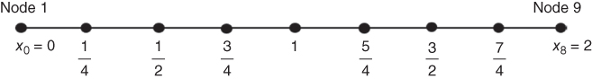
Figure 6.4 Nodal points for the domain Ω = [0, 2].
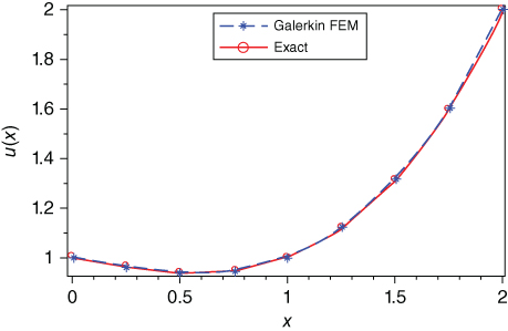
Figure 6.5 Comparison of the Galerkin FEM solution with the exact solution for Example 6.1.
6.3.2 Partial Differential Equation
In this section, the Galerkin FEM is applied to solve diffusion equation
satisfying boundary conditions u(a, t) = γa and u(b, t) = γb over the domain Ω(x, t).
The steps involved in solving diffusion equation using the Galerkin FEM are illustrated below:
Step (i): Divide the global domain Ω(x, t) into finitely m × n elements as illustrated in Figure 6.6, with respect to time step Δtj = tj − tj − 1 and element length step Δxi = xi − xi − 1. In case of equal spacing discretization, Δtj = Δt and Δxi = Δx for j = 1, 2, …, n and i = 1, 2, …, m.
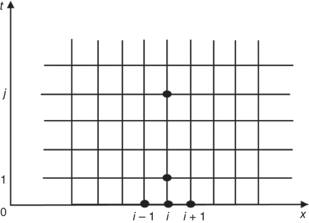
Figure 6.6 Finite‐element two‐dimensional discretization.
Step (ii): Consider the element interpolating polynomial for the global approximate solution 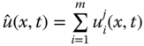 as
as
for i = 1, 2, …, m having element shape functions
Step (iii): Apply the Galerkin FEM [9] to each element i in order to obtain the corresponding element equations.
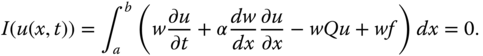
In this regard, the weighted residual integral is given as
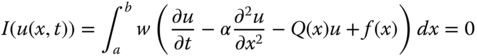
where w is the weight function and ![]() is the residual.
is the residual.
Equation (6.25) is integrated by parts such that ![]() . Here,
. Here, ![]() cancels out in all the interior nodes (except at end nodes) during assembling. As such, Eq. ( 6.25
) reduces to
cancels out in all the interior nodes (except at end nodes) during assembling. As such, Eq. ( 6.25
) reduces to
For each ith element, Eq. (6.26) reduces to element integral,
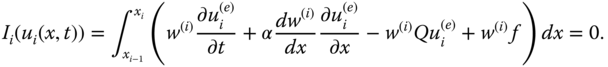
Here, Eq. (6.27) involves partial derivatives

Moreover, the weight functions in the Galerkin‐weighted residual method are considered in terms of the shape functions φi − 1(x) and φi(x) as
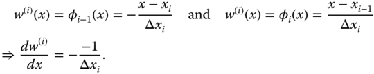
Using the weight function w(i) = φi − 1, Eq. ( 6.27 ) reduces to
where ![]() and
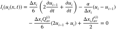
and ![]() are the average values of Q(x) and f(x), respectively, for ith element. Further, substituting w(i) = φi in Eq. ( 6.27
) results in
are the average values of Q(x) and f(x), respectively, for ith element. Further, substituting w(i) = φi in Eq. ( 6.27
) results in
Equations (6.28a) and (6.28b) are referred to as the element equations for the ith element.
Step (iv): Obtain the nodal equations by assembling the element equations at (i + 1)th node to form a system of equations with respect to unknown nodal values.
Using Eqs. (6.28a) and (6.28b), the element equations for the (i + 1)th element are
The nodal equation at the (i + 1)th node is obtained by adding Eqs. (6.28b) and (6.29a),
Using finite difference approximation ![]() for j = 1, 2, …, n, we further obtain
for j = 1, 2, …, n, we further obtain
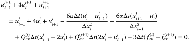
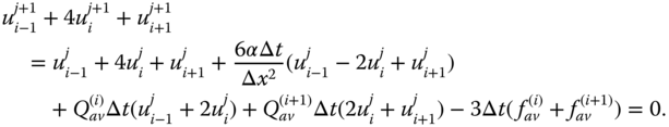
Equation (6.31) for equal spacing yields
Step (v): Adjust the obtained system of equations using the boundary conditions u(a, t) = γa and u(b, t) = γb to obtain unknown nodal values.
Table 6.1 Solution of one‐dimensional heat equation by the Galerkin FEM.
| u(x, t) | |||||
| tx | 0 | 0.25 | 0.5 | 0.75 | 1 |
| 0 | 0 | 2.1213 | 3 | 2.1213 | 0 |
| 0.02 | 0 | 1.6807 | 2.3768 | 1.6807 | 0 |
| 0.04 | 0 | 1.3315 | 1.8831 | 1.3315 | 0 |
| 0.06 | 0 | 1.0549 | 1.4919 | 1.0549 | 0 |
| 0.08 | 0 | 0.8358 | 1.1820 | 0.8358 | 0 |
| 0.1 | 0 | 0.6622 | 0.9364 | 0.6622 | 0 |
6.4 Structural Analysis Using FEM
In structural mechanics, the approximate solution of governing partial differential equations for structures may be obtained using the FEM. Under static and dynamic conditions, the associated differential equations get transformed to simultaneous algebraic equations and eigenvalue problems, respectively. In this regard, static and dynamic analysis of structural systems are considered in Sections 6.4.1 and 6.4.2 respectively.
6.4.1 Static Analysis
This section considers the FEM modeling of one‐dimensional structural system subject to static conditions. For instance, consider the simplest one‐dimensional finite‐element structure of spring or bar given in Figure 6.7.
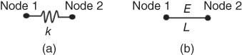
Figure 6.7 One‐element (a) spring and (b) bar.
A spring having stiffness k or bar having Young's modulus E of length L may be considered as an element having two nodes with forces f1, f2 applied on either nodes 1 and 2, respectively. The system of equations for one element spring as given in Refs. [2, 8 ] is obtained as
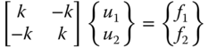
such that u1 and u2 are the nodal displacements. For one‐element bar having stiffness ![]() , the system is considered as given in Eq. (6.34) subject to axial force
, the system is considered as given in Eq. (6.34) subject to axial force ![]() , where A is the cross‐sectional area of the bar.
, where A is the cross‐sectional area of the bar.
Similarly, for n element bar given in Figure 6.8, the system of equations is obtained as
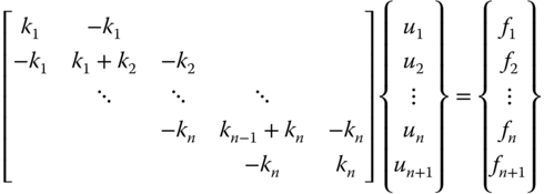
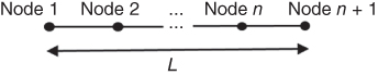
Figure 6.8 n bar element.
having element length li, modulus of elasticity Ei, and area Ai such that stiffness ![]() , for i = 1, 2, …, n + 1.
, for i = 1, 2, …, n + 1.
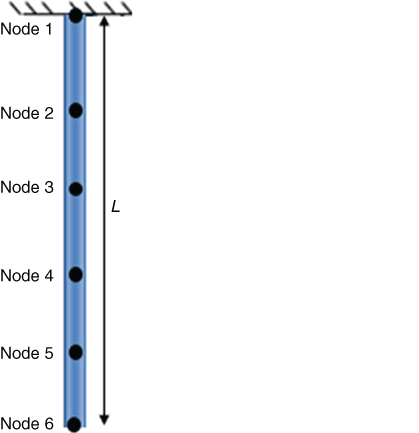
Figure 6.9 Five‐element hanging rod.
6.4.2 Dynamic Analysis
In order to incorporate the usage of the FEM in dynamic analysis of structural systems, one‐dimensional fixed free bar [2] governed by
(as depicted in Figure 6.10) is taken into consideration.
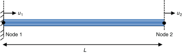
Figure 6.10 Fixed free‐bar element.
For free vibration u = Uei ωt, where U is the nodal displacement and ω is the natural frequency. Using the FEM, Eq. (6.37) gets transformed to eigenvalue problem,
Similarly, for n element bar (Figure 6.11), the eigenvalue problem gets reduced to
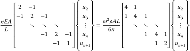
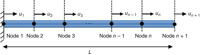
Figure 6.11 Fixed free n element bar.
Here, K and M are the stiffness and mass matrices.
Exercise
- 1 Solve boundary value problem u″ − 9u = 0, u(0) = 0, and u(1) = 10 using the Galerkin FEM.
- 2 Compute the nodal frequencies for 10‐element fixed free bar of unit length with material properties Young's modulus E = 2 × 10¹¹ N/m2, density ρ = 7800 kg/m3, and cross‐sectional area A = 30 × 10−6 m2.
References
- 1 Zienkiewicz, O.C., Taylor, R.L., and Zhu, J.Z. (2005). The Finite Element Method: Its Basis and Fundamentals, 6e, vol. 132, 1987–1993. Barcelona: Butterworth‐Heinemann.
- 2 Petyt, M. (2010). Introduction to Finite Element Vibration Analysis. New York: Cambridge University Press.
- 3 Rao, S.S. (2017). The Finite Element Method in Engineering, 6e. Oxford: Butterworth‐Heinemann.
- 4 Seshu, P. (2003). Textbook of Finite Element Analysis. New Delhi: PHI Learning Private Limited.
- 5 Bhavikatti, S.S. (2005). Finite Element Analysis. New Delhi: New Age International.
- 6 Logan, D.L. (2015). A First Course in the Finite Element Method, 6e. Boston: Cengage Learning.
- 7 Nayak, S. and Chakraverty, S. (2018). Interval Finite Element Method with MATLAB. London: Academic Press.
- 8 Gerald, C.F. and Wheatley, P.O. (2004). Applied Numerical Analysis, 7e. New Delhi: Pearson Education.
- 9 Hoffman, J.D. and Frankel, S. (2001). Numerical Methods for Engineers and Scientists, 2e. New York: McGraw‐Hill, Inc.
- 10 Jain, M.K. (2014). Numerical Solution of Differential Equations. New Delhi: New Age International.
- 11 Evans, G.A., Blackledge, J.M., and Yardley, P.D. (eds.) (2000). Finite element method for ordinary differential equations. In: Numerical Methods for Partial Differential Equations, 123–164. London: Springer.
- 12 Kattan, P.I. (2010). MATLAB Guide to Finite Elements: An Interactive Approach. New York: Springer Science and Business Media.