
20
Differential Equations with Fuzzy Uncertainty
20.1 Introduction
In this chapter, a system of fuzzy linear differential equations is studied. Recently, a new technique using the triangular fuzzy numbers (TFNs) [1,2] is illustrated to model the fuzzy linear differential equations. The solution of linear differential equations with fuzzy initial conditions may be studied as a set of intervals by varying α‐cut. The term fuzzy differential equations were first introduced by Chang and Zadeh [3,4]. Later, Bede introduced a strongly generalized differentiability of fuzzy functions in Refs. [5,6]. Recently, various researchers viz. Allahviranloo et al. [7], Chakraverty et al. [8], Tapaswini and Chakraverty [9] have studied fuzzy differential equations. As such, a geometric approach to solve fuzzy linear systems of differential equations have been studied by Gasilov et al. [ 1 , 2 ,10,11]. The difference between this method and the methods offered to handle the system of fuzzy linear differential equation is that at any time the solution consists a fuzzy region in the coordinate space. In this regard, the following section presents a procedure to solve fuzzy linear system of differential equations.
20.2 Solving Fuzzy Linear System of Differential Equations
20.2.1 α‐Cut of TFN
To understand the preliminary concepts of fuzzy set theory, one can refer Refs. [12,13]. There exist various types of fuzzy numbers and among them the TFN is found to be mostly used by different authors.
A TFN ![]() is a convex normalized fuzzy set
is a convex normalized fuzzy set ![]() of the real line ℜ [ 3
, 4
] such that,
of the real line ℜ [ 3
, 4
] such that,
- ∃ exactly one x0 ∈ R with
 where x0 is referred to as the mean value of
  and
and  is the membership function of the fuzzy set such that
  .
.  is piecewise continuous.
The membership function ![]() of
of ![]() is defined (Figure 20.1) as follows:
is defined (Figure 20.1) as follows:

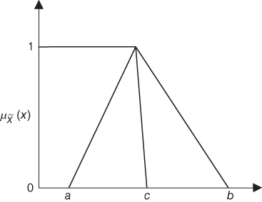
Figure 20.1 Triangular fuzzy number.
where c ≠ a and c ≠ b.
Using the α‐cut approach, the TFN ![]() can further be represented by an ordered pair of functions,
can further be represented by an ordered pair of functions, ![]() , where α ∈ [0, 1].
, where α ∈ [0, 1].
20.2.2 Fuzzy Linear System of Differential Equations (FLSDEs)
Let aij are crisp numbers, hi(t) are given crisp functions, ![]() for 0 ≤ α ≤ 1, and 1 ≤ i, j ≤ n, (are fuzzy numbers). Fuzzy Linear System of Differential Equations (FLSDEs) [ 1
, 2
] may be written as
for 0 ≤ α ≤ 1, and 1 ≤ i, j ≤ n, (are fuzzy numbers). Fuzzy Linear System of Differential Equations (FLSDEs) [ 1
, 2
] may be written as

subject to the fuzzy initial conditions
One can formulate Eqs. (20.1) and (20.2) in matrix notation as follows:

where A = (aij) is n × n crisp matrix, H(t) = (h1(t), h2(t), …, hn(t))T is the crisp vector function, and ![]() is the vector of fuzzy numbers.
is the vector of fuzzy numbers.
20.2.3 Solution Procedure for FLSDE
Let us express the initial condition vector as ![]() , where (bcr)i denotes the crisp part of
, where (bcr)i denotes the crisp part of ![]() and
and ![]() denotes the uncertain part. Solution of such system may be considered of the form
denotes the uncertain part. Solution of such system may be considered of the form ![]() (crisp solution + uncertainty). Here, xcr(t) is a solution of the nonhomogeneous crisp problem as given in Refs. [ 1
, 2
]
(crisp solution + uncertainty). Here, xcr(t) is a solution of the nonhomogeneous crisp problem as given in Refs. [ 1
, 2
]

whereas ![]() is the solution of the homogeneous system with fuzzy initial conditions,
is the solution of the homogeneous system with fuzzy initial conditions,

It is possible to compute xcr(t) by means of known analytical or numerical methods. Our aim is to solve Eq. (20.3) with fuzzy initial conditions. In this regard, fuzzy uncertainty in terms of TFN is taken into consideration. Let ![]() be the TFN, then
be the TFN, then ![]() is written as
is written as ![]() , where qi designates the crisp part and
, where qi designates the crisp part and ![]() designates the TFN.
designates the TFN.
Below, we present an example problem for clear understanding of the described method.

Figure 20.2 Triangular solution of x(t) for α = 0 : 0.1 : 1 at t = 1.
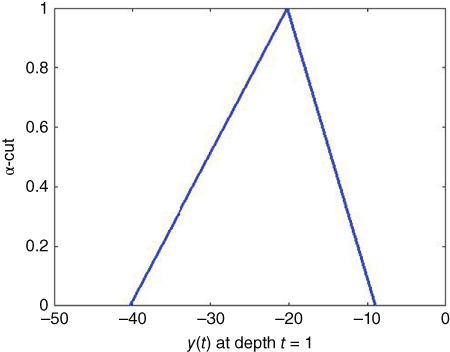
Figure 20.3 Triangular solution of y(t) for α = 0 : 0.1 : 1 at t = 1.
Exercise
Solve the following system of differential equations:
- 1

- 2

- 3

References
- 1 Gasilov, N., Amrahov, S.G., and Fatullayev, A.G. (2011). A geometric approach to solve fuzzy linear systems of differential equations. Applied Mathematics and Information Sciences 5: 484–499.
- 2 Gasilov, N., Amrahov, Ş.E., Fatullayev, A.G. et al. (2011). A geometric approach to solve fuzzy linear systems. CMES: Computer Modeling in Engineering and Sciences 75: 189–203.
- 3 Chang, S.S. and Zadeh, L.A. (1996). On fuzzy mapping and control. In: Fuzzy Sets, Fuzzy Logic, and Fuzzy Systems: Selected Papers by Lotfi A. Zadeh (ed. G.J. Klir and B. Yuan), 180–184. River Edge, NJ: World Scientific Publishing Co., Inc.
- 4 Kandel, A. and Byatt, W.J. (2078). Fuzzy sets, fuzzy algebra, and fuzzy statistics. Proceedings of the IEEE 66 (12): 1620–1639.
- 5 Bede, B. and Gal, S.G. (2005). Generalizations of the differentiability of fuzzy‐number‐valued functions with applications to fuzzy differential equations. Fuzzy Sets and Systems 151 (3): 581–599.
- 6 Hukuhara, M. (2067). Integration des applications mesurables dont la valeur est un compact convexe. Funkcialaj Ekvacioj 10 (3): 205–223.
- 7 Allahviranloo, T., Kiani, N.A., and Motamedi, N. (2009). Solving fuzzy differential equations by differential transformation method. Information Sciences 179 (7): 956–966.
- 8 Chakraverty, S., Tapaswini, S., and Behera, D. (2016). Fuzzy Differential Equations and Applications for Engineers and Scientists. Boca Raton, FL: CRC Press.
- 9 Tapaswini, S. and Chakraverty, S. (2014). New analytical method for solving n‐th order fuzzy differential equations. Annals of Fuzzy Mathematics and Informatics 8: 231–244.
- 10 Mandal, N.K., Roy, T.K., and Maiti, M. (2005). Multi‐objective fuzzy inventory model with three constraints: a geometric programming approach. Fuzzy Sets and Systems 150 (1): 87–106.
- 11 Gasilov, N., Amrahov, S.E., Fatullayev, A.G. et al. (2012). Application of geometric approach for fuzzy linear systems to a fuzzy input‐output analysis. Computer Modeling in Engineering and Sciences(CMES) 88 (2): 93–106.
- 12 Zimmermann, H.J. (2010). Fuzzy set theory. Wiley Interdisciplinary Reviews: Computational Statistics 2 (3): 317–332.
- 13 Moore, R. and Lodwick, W. (2003). Interval analysis and fuzzy set theory. Fuzzy Sets and Systems 135 (1): 5–9.