Search in book...
Toggle Font Controls
Create new playlist

Name your new playlist

Playlist description (optional)
Sign In

Email address

Password

Forgot Password?

or

Continue with Facebook

Continue with Google
Sign Up

Full Name

Email address

Confirm Email Address

Password

or

Continue with Facebook

Continue with Google

14
Homotopy Analysis Method

14.1 Introduction

Homotopy analysis method (HAM) [1–7] is one of the well‐known semi‐analytical methods for solving various types of linear and nonlinear differential equations (ordinary as well as partial). This method is based on coupling of the traditional perturbation method and homotopy in topology. By this method one may get exact solution or a power series solution which converges in general to exact solution. The HAM consists of parameter ℏ ≠ 0 called as convergence control parameter, which controls the convergent region and rate of convergence of the series solution. This method was first proposed by Liao [4]. The same was successfully employed to solve many types of problems in science and engineering [ 1 –8] and the references mentioned therein.

14.2 HAM Procedure

To illustrate the idea of HAM, we consider the following differential equation 1– 7 ] in general

(14.1)

where N is the operator (linear or nonlinear) and u is the unknown function in the domain Ω.

The method begins by defining homotopy operator H as below [7] ,

(14.2)

where p ∈ [0, 1] is an embedding parameter and ℏ ≠ 0 is the convergence control parameter [3, 7 ], u₀ is an initial approximation of the solution of Eq. (14.1), φ is an unknown function, and L is the auxiliary linear operator satisfying the property L(0) = 0.

By considering H(φ, p) = 0, we obtain

(14.3)

which is called the zero‐order deformation equation.

From Eq. (14.3), it is clear that for p = 0 we get L(φ(x, t; 0)) − u₀(x, t) = 0 that gives φ(x; 0) = u₀(x, t). On the other hand, for p = 1, Eq. ( 14.3 ) reduces to N(φ(x, t; p)) = 0 which gives φ(x, t; 1) = u(x). So, by changing p from 0 to 1 the solution changes from u₀ to u.

Using Maclaurin series, the function φ(x, t; p) with parameter p may be written as [7]

(14.4)

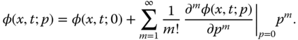
Denoting

(14.5)

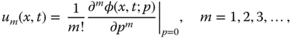
Eq. (14.4) turns into

(14.6)

If the series (14.6) converges for p = 1 [7] , then we obtain the solution of Eq. ( 14.1 ) as

(14.7)

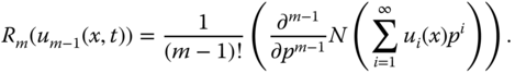
In order to determine the function u_m, we differentiate Eq. ( 14.3 ), m times with respect to p. Next we divide the result by m! and substitute p = 0 [7] . In this way we may find the mth‐order deformation equation for m > 0 as below [7]

(14.8)

where H(x, t) is the auxiliary function, images and

(14.9)

14.3 Numerical Examples

Here, we apply the present method to solve a linear partial differential equation in Example 14.1 and a nonlinear partial differential equation in Example 14.2.

Example 14.1

We consider a homogeneous linear partial differential equation from

(14.10)

subject to the initial condition u(x, 0) = e^−x.

Solution

Here, the auxiliary linear operator is .

Using the above‐discussed HAM, the zeroth‐order deformation equation is (from Eq. ( 14.3 ))

14.11

subject to the initial condition

where p ∈ [0, 1]. Obviously, if we take p = 0 we get φ(x, t; 0) = e^−x and when p = 1 the equation is equivalent to Eq. (14.10). Thus, it holds

where

(14.12)

The mth‐order deformation equation is [5, 7 , 8 ]

(14.13)

subject to

where

and

(14.14)

Let H(x, t) = 1, then Eq. (14.13) may be rewritten as

where L⁻¹ is the inverse linear differential operator.

Let u₀(x, t) = u(x, 0) = e^−x

The final solution of Eq. ( 14.10 ) is

The approximate solution plots of Eq. ( 14.10 ) of order 6 (u(x, t) = u₀(x, t) + u₁(x, t) + u₂(x, t) + u₃(x, t) + u₄(x, t) + u₅(x, t) + u₆(x, t)) for ℏ = − 0.5, − 0.8,− 1.0, − 1.2 are depicted in Figure 14.1 and also one may see the comparison of present results with exact solution at t = 1. Similarly Figure 14.2 represents the same type of results for ℏ = − 0.5, − 0.7, − 0.8, − 1.0 at t = 2.

Here, the exact solution of Eq. ( 14.10 ) is u(x, t) = e^−x + t.

From the results presented in Figure 14.1 , one may see that for ℏ = − 1.0 the HAM solution is exactly the same as exact solution. The solution for ℏ = − 0.80 is also converging to exact solution. Figure 14.2 also confirms that for t = 2, the HAM solution is converging to exact solution for ℏ = − 1.2. From the above discussion it may be concluded that proper values of control parameter ℏ should be chosen for getting better solution with less error. It may be noted that the HAM not only produces approximate convergent series solution but it can also give exact solution depending on the considered problem with proper ℏ. This may be observed in the next example.

Graph of solution u(x,1) vs. x displaying descending curves with markers for exact, HAM for h = -0.50, HAM for h = -0.70, HAM for h = -0.80, and HAM for h = -1.0. — Figure 14.1 Solution of Eq. ( 14.10 ) for different values of ℏ at t = 1.

Example 14.2

Now, we take a nonlinear and nonhomogeneous advection equation [9] as

(14.15)

subject to the initial condition u(x, 0) = 2.

The zeroth order deformation equation in this case is

14.16

subject to

where p ∈ [0, 1]. Obviously, if we take p = 0 we get (x, t; 0) = 2 and when p = 1 the equation is equivalent to Eq. (14.15). Thus, it holds φ(x, t; 1) = u(x, t).

The Taylor series expansion of φ(x, t; p) is

(14.17)

By substituting Eq. (14.17) into Eq. (14.16) and equating the coefficients of like powers of p, the mth‐order deformation equation may be obtained as below [8]

(14.18)

Subject to u_m(x, 0) = 0

For H(x, t) = 1, the solution of the mth‐order deformation equation 14.18) reads as

(14.19)

where

and

(14.20)

Let u₀(x, t) = u(x, 0) = 2

So, the solution of Eq. ( 14.15 ) up to three terms is

One may see that for ℏ = − 1,

which is same as the exact solution [9] .

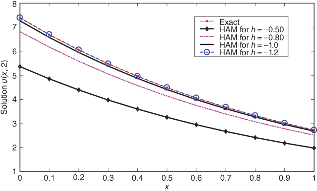
Graph of solution u(x,2) vs. x displaying descending curves with markers for exact, HAM for h = -0.50, HAM for h = -0.80, HAM for h = -1.0, and HAM for h = -1.2. — Figure 14.2 Solution of Eq. ( 14.10 ) for different values of ℏ at t = 2.

Exercise

1 Apply the HAM to find the solution of the partial differential equation , subject to the initial condition u(x, 0) = 0.
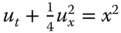
2 Find the solution of u_t + uu_t = x² subject to .

References

1 Wazwaz, A.M. (2008). A study on linear and nonlinear Schrodinger equations by the variational iteration method. Chaos, Solitons and Fractals 37 (4): 1136–1142.
2 Song, L. and Zhang, H. (2007). Application of homotopy analysis method to fractional KdV–Burgers–Kuramoto equation. Physics Letters A 367 (1): 88–94.
3 Liao, S. (2004). On the homotopy analysis method for nonlinear problems. Applied Mathematics and Computation 147 (2): 499–513.
4 Liao, S. (2012). Homotopy Analysis Method in Nonlinear Differential Equations, 153–165. Beijing: Higher Education Press.
5 Liang, S. and Jeffrey, D.J. (2009). Comparison of homotopy analysis method and homotopy perturbation method through an evolution equation. Communications in Nonlinear Science and Numerical Simulation 14 (12): 4057–4064.
6 Abbasbandy, S. (2006). The application of homotopy analysis method to nonlinear equations arising in heat transfer. Physics Letters A 360 (1): 109–113.
7 Hetmaniok, E., Słota, D., Trawiński, T., and Wituła, R. (2014). Usage of the homotopy analysis method for solving the nonlinear and linear integral equations of the second kind. Numerical Algorithms 67 (1): 163–185.
8 Liao, S.J., 1992. The proposed homotopy analysis technique for the solution of nonlinear problems. Doctoral dissertation, PhD thesis, Shanghai Jiao Tong University.
9 Wazwaz, A.M. (2010). Partial Differential Equations and Solitary Waves Theory. Beijing: Springer Science & Business Media, Higher Education Press.

..................Content has been hidden....................

You can't read the all page of ebook, please click here login for view all page.

Table of Contents for 14 Homotopy Analysis Method

Create new playlist

Sign In

Sign Up

14.1 Introduction

14.2 HAM Procedure

14.3 Numerical Examples

Exercise

References

Table of Contents for
14 Homotopy Analysis Method