
2
Integral Transforms
2.1 Introduction
In Chapter 1, we have discussed about basic numerical methods by which one may find the approximate solutions of ordinary differential equations. In this regard, this chapter deals with the exact solutions of ordinary and partial differential equations. The methods we discuss here are integral transform methods. These are used frequently in different fields of engineering and sciences. Especially, Laplace transform (LT) and Fourier transform (FT) are having wide range of applications. Although one may find theories, concepts, and details about these methods in different excellent books [1–8]. But, just to have an idea of these methods, we introduce here the basic concepts of LT and FT. Accordingly, in this chapter, we will address these two methods LT and FT for solving ordinary and partial differential equations.
Integral transform of a function f(t) is defined as below:
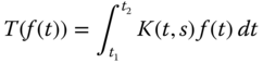
where K(t, s) is called kernel of the transformation.
2.2 Laplace Transform
LT is a well‐known integral transform method.
In other way, one may define as below:
If the kernel in Eq. (2.1) is K(t, s) = e−st, then the integral transform is called as LT.
The list of few formulae and properties of LT that are useful in further discussion are given in Table 2.1 which may easily be obtained using Definition 2.1.
Table 2.1 Laplace transforms of f(t).
| S. no | f(t) = ℒ−1{F(s)} | F(s) = ℒ{f(t)} |
| 1 | 1 | |
| 2 | tn, n = 1, 2, 3, … | |
| 3 | eat | |
| 4 | cos(at) | |
| 5 | sin(at) | |
| 6 | eatf(t) | F(s − a) |
| 7 | tnf(t) |  |
| 8 | Linear property: ℒ{af(t) + bg(t)} = aℒ{f(t)} + bℒ{g(t)} | |
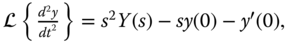
| 9 | LT of nth derivative is ℒ{yn(t)} = snY(s) − sn − 1y(0) − sn − 2y′(0) − ⋯ − yn − 1(0), where y(0), y′(0), … are initial conditions and Y(s)= ℒ{y(t)} | |
Further details of LT and its applications to various engineering and science problems are available in standard books [ 1 –3,6].
2.2.1 Solution of Differential Equations Using Laplace Transforms
In this section we study how to use LT for solving ordinary and partial differential equations with the help of three examples. First, we briefly explain how to solve initial value problems using LT [ 1 , 2 ].
Let us consider a second order linear ordinary differential equation as below:
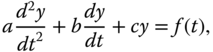
with initial conditions y(0) = d, y′(0) = e.
The basic steps involved in solving Eq. (2.3) using LT are discussed below:
- Step (i): Take LT on both sides of the differential equation 2.3).
- Step (ii): Using differentiation property of LT (Table 2.1
)
 ,
,  and initial conditions, we obtain Y(s) in terms of s.
 - Step (iii): Find the inverse LT of Y(s) to get the solution of the initial value problem.
One may solve higher‐order differential equations also in the similar fashion. We now consider a simple initial‐value problem to understand the solution procedure of the method.
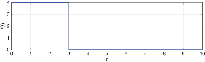
Figure 2.1 Plot of the function f(t) = 4(1 − u3(t)).
2.3 Fourier Transform
FT is another well‐known integral transform method like LT for solving differential equations.
In other way, one may define as below:
If the kernel in Eq. ( 2.1 ) is K(t, s) = eist, then the integral transform is called as FT.
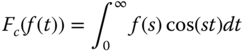
If f(t) is an even function, then the FT is called as cosine FT and the same is given as
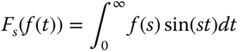
Similarly, if f(t) is an odd function, then we have sine FT and it is written as
In this regard, FTs of some standard functions are presented in Table 2.2.
Table 2.2 Fourier transforms.
| S. no. | Function | Fourier transform |
| 1 | Delta function δ(x) | 1 |
| 2 | Exponential function e−a|x| | |
| 3 | Gaussian |
|
| 4 | Derivative f′(x) | isF(s) |
| 5 | Convolution property: f(x) * g(x)a | F(s)G(s) |
| 6 | nth derivative |
(2πis)nF(s) |
| 7 | nth partial derivative |
(is)nU(s, t) |
| 8 | nth partial derivative |
aConvolution of f(x) and g(x) is ![]() .
.
Here, F(s), G(s), and U(s, t) are the FTs of f(x), g(x), and u(x, t) respectively.
2.3.1 Solution of Partial Differential Equations Using Fourier Transforms
Solution of partial differential equations using FTs [2] is briefly explained below.
- Step (i): First, apply FT on both sides of the given partial differential equation.
- Step (ii): Use the derivative property of FT to find the FT of partial derivative as below (see Table 2.2 ):
and
- then simplify algebraically to obtain ordinary differential equation with independent variable t.
- Step (iii): Solve the above obtained ordinary differential equation to get U(s, t).
- Step (iv): Find the inverse FT of U(s, t) to obtain u(x, t) which is the solution of the given differential equation.
Exercise
- 1
Use LT to solve the below initial value problems
- y″ + y = 2 cos(t), y(0) = 3, y′(0) = 4

- y″ − y′ − 2y = 12uπ(t) sin(t), y(0) = 1, y′(0) = − 1
- 2 Solve the given partial differential equation using LT ut + ux = 0, x > 0, t > 0 subject to the conditions u(x, 0) = sin(x), u(0, t) = 0.
References
- 1 Widder, D.V. (2015). Laplace Transforms (PMS‐6). Princeton, NJ: Princeton University Press.
- 2 Beerends, R.J., ter Morsche, H.G., van den Berg, J.C., and van de Vrie, E.M. (2003). Fourier and Laplace Transforms. Cambridge: Cambridge University Press Translated from the 1992 Dutch edition by Beerends.
- 3 Duffy, D.G. (2004). Transform Methods for Solving Partial Differential Equations. Boca Raton, FL: Chapman and Hall/CRC.
- 4 Bracewell, R.N. and Bracewell, R.N. (1986). The Fourier Transform and Its Applications, vol. 31999. New York: McGraw‐Hill.
- 5 Haberman, R. (1983). Elementary Applied Partial Differential Equations: With Fourier Series and Boundary Value Problems. Upper Saddle River, NJ: Prentice Hall.
- 6 Spiegel, M.R. (1965). Laplace Transforms. New York: McGraw‐Hill.
- 7 Marks, R.J. (2009). Handbook of Fourier Analysis and Its Applications. Oxford: Oxford University Press.
- 8 Poularikas, A.D. (2010). Transforms and Applications Handbook. Boca Raton, FL: CRC Press.
- 9 Kreyszig, E. (2010). Advanced Engineering Mathematics. New Delhi: Wiley.