
Chapter 7
Estimating and Segmenting Projects
Why do development teams frequently overcommit and how does agile’s “sized-based estimation” avoid this trap?
How can story points and project backlog enable us to predict how long a project will take and how much it will cost?
How can we group the estimated components into major deliverables, given that we cannot build everything at once?
All software development teams must estimate labor requirements in order to plan their work and communicate project trajectories effectively with their stakeholders. Although no software developer can predict the level of effort work units will demand with perfect certainty, accuracy in estimation is worth some study and effort because the more dependable a team can make its estimates, the easier it will be for them to deliver according to the resulting plan. Accurate estimating also lessens the chance a team will have to disappoint project stakeholders with schedule and cost overruns.
Previous chapters detailed an agile approach to defining projects with just enough detail to understand the work required, both at the outset of an effort and then repeatedly before each development iteration. The result of that definition process provides a backlog defined at two levels: First from a business perspective, the backlog begins with “user stories” authored by the team’s product owner. Second, this backlog also contains a decomposition of those user stories into “developer stories” that are small and technically explicit enough that developers on the team can begin delivering the required system components. As presented in this chapter, agile provides a novel technique called “size-based estimation” for predicting the level of effort the stories on a backlog will require. Teams can employ this new technique upon only the leading edge of the backlog in order to define just the next iteration. They can also use the technique to estimate the entire backlog in order to forecast the labor a complete release or full project will require.
Once the backlogs are estimated, data warehousing teams will naturally want to group the components of work into iterations and releases. Teams can draw upon three techniques for assembling the developer stories on a project backlog into both reasonably scoped iterations and a series of releases that will provide end users with a steady stream of valuable business analytics. Compared to the estimating approach taken by waterfall projects, agile estimation is mentally easier and repeated far more frequently as part of the method, allowing teams to forecast a project’s labor requirements far more dependably. This ability to estimate accurately requires both a solid understanding of the work implicit within a project and a well-tune delivery process. Because failings in any part of this chain will prevent the team from delivering as promised, the agile team can employ the accuracy of their estimates as a highly sensitive metric for tracking the quality of a team’s overall delivery process.
Failure of traditional estimation techniques
The Standish Group’s Chaos reports, published before agile techniques were common, documented that less than one-third of information technology (IT) projects over $750 K are implemented on time, within budget, and with all the features promised. The reports cited “underestimating project complexity and ignoring changing requirements” as basic reasons why these projects failed. [Standish 1999] Such findings clearly suggest that if developers receive only one chance to estimate a project, they will rarely forecast accurately, allowing sponsors to expect far too much functionality while budgeting far too little funding for the project. Despite the growing sophistication of our industry, inaccurate estimates continue to vex information systems groups, leading one long-time observer to sadly ask “How can experts know so much and predict so badly?” [Camerer 1991]
Empirical evidence shows that developers forecast only half the effort their tasks will take, with a large amount of skew in the distribution above this mean. [Demarco 1982; Little 2004] Figure 7.1 shows this distribution and provides an instant insight as to why traditional estimation techniques regularly undermine project success. To understand this dynamic, one must keep in mind that project sponsors and managers absolutely despise exceeding their budgets and can make life very unpleasant for developers when a project threatens to do so. However, the long tail to the right in Figure 7.1 reveals that these managers should be requesting not twice, but four times as much funding as the team estimates in order to be 95% confident they will not have to make “another trip to the well.”
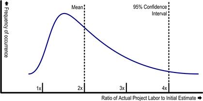
Figure 7.1 Empirically, waterfall estimates are difficult to rely upon.
Few managers are willing to quadruple their project estimates, yet when they only double their team’s labor projections, they instill unavoidable disappointment into the future of at least every other project. Somewhere long before the expected delivery date, these projects are going to appear undoable as defined. Developers will be pressured into making heroic efforts involving working nights and weekends. Quality, moderately neglected as soon as overtime started, continues to fall as developer morale sinks. The cost of the overtime work will exceed the project budget long before the first release sees production, resulting in unhappy project sponsors. Scope will be cut in order to restore some measure of feasibility, adding horrified customers to the disgruntled sponsors. Downstream teams that had been depending on the project to deliver will find important prerequisites for their applications delivered late with less than expected scope. All this pain occurs because, as revealed in Figure 7.1, traditional estimating is congenitally blind to the time and resources a software project truly needs.
As the logistical, financial, and political strains of an underfunded project reverberate throughout the company, the organization enters, crisis by crisis, the “disappointment cycle” sketched in Chapter 1. The project’s final costs ends up greatly exceeding the value delivered. At the project postmortem, frustration and conflict will swell as the team zeroes in on the root cause of the problem, one that many of them had seen before: “Why did we promise again to metaphorically force 10 pounds of fruit into a 5-pound sack?”
Traditional estimating strategies
What are the estimating approaches used by traditional projects that perform so poorly? The profession has taken two main strategies for forecasting level of effort: formal estimation models and expert judgment. Formal estimation models are parameter-driven formulas that supposedly will predict, when provided sufficient measures describing the software envisioned, both a mean and a variance for the level of effort required to build it. Expert judgment, however, involves providing a system description to experienced systems professionals, then relying upon their intuition to provide a probable labor estimate and a range of uncertainty.
Formal estimation models are appealing because they seem to encapsulate years of lessons learned into formulas that one can inspect and fine-tune. In practice, however, such models have been expensive to build and disappointing in results for the simple reason that, for all their cost, they are no more accurate than expert judgment. One survey of a hundred IEEE papers regarding software effort estimation methods indicated that “…estimation models are very inaccurate when evaluated on historical software projects different from the project on which [they] were derived.” [Jorgensen 2000] Unfortunately for data warehouse projects, business intelligence applications within a given company differ constantly from previous efforts due to evolving sources systems, innovation in tools, and the diversity of business areas within an enterprise.
A second reason that formal models often disappoint their sponsors is that software engineers will subvert them once they become too complex to understand readily. The author has observed many instances where engineers became frustrated while working with complex estimating spreadsheets with thousands of cells. Instead of requesting an update to the logic of the estimating utility, these users would simply open a hidden worksheet of the tool and overwrite an intermediate result with a value they found more believable. In choosing an estimating approach, planners must accept that the entirety of an estimating technique must remain easily intelligible to the staff members employing it, or they will simply draw upon their intuition, often without much discipline to their approach.
If the effectiveness of formal estimating models is limited, then one must rely upon expert judgment. To its credit, expert judgment can be deployed in very short order and “… seems to be more accurate when there [is] important domain knowledge not included in the estimation models, [or] when the estimation uncertainty is high as a result of environmental changes….” [Jorgensen 2004] Traditional project management offers several methods for gathering input from many individuals and collating it into an expert judgment forecast. Some of these methods can yield reliable estimates if followed carefully.
Business pressures frequently undermine these more disciplined methods, however. Instead of being asked to follow a careful, deliberate approach, developers are ordered more frequently to produce an estimate by an arbitrarily close calendar date. Faced with a tight deadline, developers will gather into a single conference room and “hammer out” an estimate for management as fast as possible. This approach can be called the estimating bash, where developers simultaneously draft a project’s work breakdown structure and forecast the work effort required, task by task, using any means they see fit.
Some projects make an effort to gather expert judgment in a more deliberative style. They parcel out aspects of the project to individual developers and then invite them to present their findings at a consolidation meeting. Although the prep work was performed carefully, the collation process involves reviewing the reasonableness of the component estimates. This consolidation meeting often becomes just another estimating bash as folks challenge each other’s forecasts over a conference table and revise them based on hasty, not-so-expert judgments. Given that the failure rates documented by the Chaos reports actually increased with the size of projects, this consolidation process appears to be just as vulnerable to the unreliable, ad hoc techniques that dominate the estimation process of small projects.
Why waterfall teams underestimate
What are the dynamics occurring in projects large and small that push traditional projects into the grave underestimates considered earlier? Four counterproductive patterns are regularly at work: single-pass efforts, insufficient feedback, rewards for overoptimism, and few reality checks.
A single-pass effort
According to the Project Management Institute’s (PMI) outline of the standard waterfall practice, planners should work through a series of cost estimates as they envision, fund, and finally plan their projects in detail. PMI expects project managers to work with software engineers to produce and estimate a “work breakdown structure” (WBS). Forecasts based on these WBS should start as order of magnitude predictions (–25 to +75% accuracy) and eventually become definitive estimates (–5 to +10%). [PMI 2008] Only once the team has produced a detailed WBS and a definitive estimate can development work begin. The project manager will employ this last work breakdown and estimate as a comprehensive project plan to which he will doggedly keep the project team aligned. When cost and schedule overruns grow too large, he will be forced to “rebaseline” the plan, but, because hard and fast promises to stakeholders were based on this “definitive estimate,” such adjustments are made only rarely.
In this common approach to development projects, labor estimation is something developers are asked to do only once in a long while. Producing a definitive WBS is tedious work, and many months pass before the project concludes and estimators discover how well their forecasts matched actual results. Given these factors, developers naturally view accurate estimation as a secondary priority requirement for their careers, nowhere near as important as technical skills and even political acumen.
Project managers essentially discount estimation also because of this single-pass approach. Obtaining an estimate from the development team is simply a milestone that must be achieved before they can finish their proposals and hold a project kickoff. They approach the developers with a detectable emphasis on getting the estimate done quickly so it can be presented at the next steering committee meeting, often giving the team insufficient time to make a proper assessment. Furthermore, estimation is a cost, and once a (supposedly accurate) estimate is in hand, there seems to be little reward in continuing to invest in an effort that has already delivered its payload. Like developers, management sees estimation as something done rarely—an occasional, necessary evil.
Insufficient feedback
In the single-pass approach, the reward for estimating well is remote and indirect. Accuracy in these forecasts is measurable only many months later as the system approaches implementation. Because the actual work eventually involves a mix of tasks very different from those foreseen, the quality of the many small predictions that went into the overall forecast is difficult to ascertain. Tallies of actual labor hours eventually arrive, but they are usually aggregated across major components so that the root cause for forecasting errors ends up hidden in averages and standard deviations. Furthermore, troubled projects often get cut in scope, making it impossible for developers to match much of their earlier level-of-effort forecasts to the project actuals. In this context, little natural learning occurs and the developers cannot improve at estimating.
Moreover, the slow and obscured feedback on the quality of their labor projections means that the developers are not subject to forces encouraging accuracy in estimation. Developers, working line by line through a tedious work breakdown during an estimating bash, must envision in detail the steps required to complete each task before they can consider how long that work will take. Processing such details is possible for a small number of components, but envisioning the hundreds of items comprising a typical project consistently is beyond the capabilities of most developers. As mental fatigue sets in, what immediate consequence keeps them from estimating each subsequent task a little less carefully? As teams tire half-way through their first pass on estimating a large project, the urge to finish up eventually outweighs their wish to be thorough. They rush through the rest of the list and, thrilled to be done with such tedium, making little effort to conscientiously cross-check the results.
Overoptimism rewarded
Compounding the inaccuracies introduced by a single-pass context with little effective feedback, developers feel pressure to whittle down their best guess at labor requirements for several reasons. Whether projects are proposed to internal boards or external customers, everyone involved with the estimate realizes that too high a tally will cause the proposal to be rejected. Consequently, a “price-to-win” mentality takes over where each developer begins quoting each task at the largest acceptable estimate that the organization will accept. This approach avoids many microconflicts with the project manager organizing the estimation effort. These managers often arrive at the estimating bash with strong opinions on how long most efforts should take and can wield autocratic powers to override the estimates provided by developers. Even worse, research has documented that managers view high estimates not as an indication that the project may be too ambitious, but rather as a signal that the developers are less qualified than they should be. Surprisingly, these executives do not correct this misconception when the lower estimates turn out be wrong. [Jorgensen & Sjoberg 2006] Over the years, developers learn of this bias and become reluctant to forecast accurately because of the negative consequences such estimates send.
Few reality checks
The factors just discussed combine to give preeminence to the overly confident participants within a team. There may be several bright developers in the group who can see the enormous harm that bad estimates can cause, but there are some powerful forces that keep them from correcting the situation when one or two dominant teammates take over the estimating process.
As research has shown, the problem with incompetent people is that they lack the ability to recognize their own incompetence, a blindness that allows a highly assertive developer to thrust upon a team his hasty estimates for each task. [Goode 2000] Lamentably, groups engaged in a shared effort such as estimating under a time pressure often fail to push back upon improper impulses due to group think. Group think is defined as a “mode of thinking that people engage in when they are deeply involved in a cohesive in-group, when the members’ strivings for unanimity override their motivation to realistically appraise alternative courses of action.” [Janis 1971] Whereas many would expect a project manager to guard the team against this unfortunate pack mentality, her priority is typically to get the estimate done, and the same research defining group think revealed that “directive leadership” from the top of the group’s hierarchy usually exacerbates the problem.
Conscientious members of the estimation team may wish to correct the error-prone process unfolding within an estimating bash, but they typically have no alternative to propose because many organizations do not teach a standard estimation process or at least one robust enough to undercut dynamics as pernicious as overconfidence and group think.
Criteria for a better estimating approach
Agile practitioners have innovated upon labor estimation considerably in order to address the weakness in the approach waterfall projects typically employ. Given the pivotal role that forecasting effort plays in setting stakeholder expectations, it is not surprising that several thought leaders have studied labor estimation in great depth. Over the years, research has amassed more than a hundred possible improvements for the practice. Recently, one researcher was kind enough to consolidate them into 12 key recommendations. These recommendations are listed in Table 7.1, along with aspects of agile data warehousing that align with each recommendation. A moment’s reflection will reveal that agile’s methodological elements, and the estimating techniques explored shortly later, incorporate well all of these lessons learned.
Table 7.1 Twelve Objectives for Good Estimationa
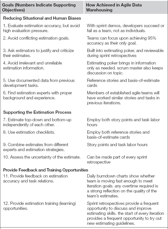
aAdapted from [Jorgensen 2004].
In general, there are four primary objectives that agile estimation must support. First, Scrum teams must estimate the top of a backlog in order to decide how many user or developer stories to take on during the next iteration. Second, most teams need to estimate an entire project during the inception phase of a project in order to secure go-ahead approval and necessary funding. Third, throughout the construction phase of a project, teams must revisit their whole project estimates in order to confirm for stakeholders that the project is still doable. Fourth, when the backlog must be changed, teams must be able to tell stakeholders the impact of including or excluding any number of stories from the backlog.
These objectives certainly drive the agile estimating approach presented here. Agile’s new approach to labor forecasting includes several innovations. First, it adds size-based estimation to complement the labor-hour forecasts, whereas waterfall methods restrict themselves only to labor-hour estimates. The size-based technique, which is presented in a moment, offers the team greater speed, accuracy, and validation for its labor forecasts.
Second, the agile approach involves frequent estimating sessions instead of following waterfall’s style of a single estimate at project start and perhaps a couple further estimates when the project has veered so far from plan that the entire forecast must be “rebaselined.” In contrast, agile includes estimation as part of every iteration, and this frequent repetition causes developers to get good at estimating quickly, and then keeps them good at that skill.
Third, agile estimation requires that teams steadily accumulate their project experience into selecting key reference stories and standardizing developer task lists for important, frequently repeated types of work. These references help developers improve estimation accuracy by encouraging them to apply project knowledge they already possess consistently.
Fourth, agile estimation cross-checks the leading edge of its story point estimates with the labor-hour forecasts for each iteration. This practice asks the team to perform two passes at forecasting the same work, each done in a different unit of measure. Developers naturally reflect upon and resolve any conflicts between the estimates, revealing for them any errors in their approach to forecasting labor.
Finally, agile estimation provides prompt and thorough feedback on the accuracy of developers’ estimates. By comparing the actual labor an iteration consumed versus the forecast the team had made a few weeks earlier, developers can steadily improve their estimating accuracy.
An agile estimation approach
All told, agile estimation addresses the weaknesses observed in the waterfall approach; as a result, agile labor forecasts throughout a project prove to be far more accurate than observed for traditional projects. In effect, agile estimation narrows the curve of actual labor versus initial estimates shown in Figure 7.1, reducing the problem of the fat tail to the right. The increased accuracy of agile forecasts allows teams to avoid overcommitment on both an iteration and a project level, while simultaneously giving management the information they need to fund and coordinate properly across multiple projects. Because estimating within an iteration is more different than estimating a full iteration, both deserve to be presented separately.
Estimating within the iteration
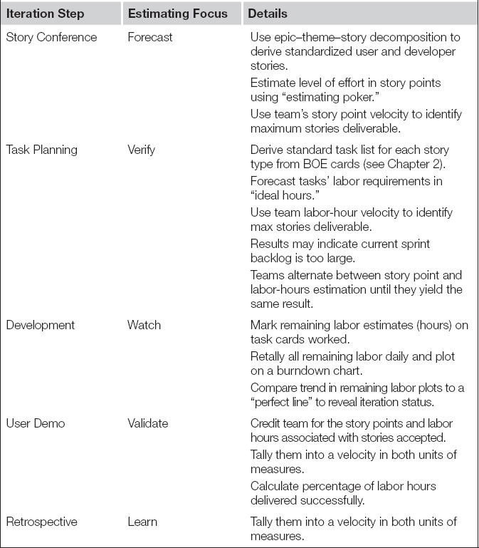
The agile approach is rooted, naturally enough, within the development iterations. Table 7.2 shows how each phase of the normal sprint incorporates estimation. The team performs a top-down forecast for only the handful of stories requested by the product owner during the story conference. As discussed in the prior chapter, these items will be user stories for front-end modules and developer stories for data integration work. Estimates made during the story conference will be in story points, first introduced in Chapter 2. When the team moves into the task planning phase of the sprint, they break the candidate stories into development tasks and estimate those work items in labor hours, that is, the total developer time required to complete the work identified by the task. For the major development modules that they must deliver frequently, agile warehousing teams will often gather a typical list of tasks and approximate labor hours onto basis-of-estimate (BOE) cards, also described in Chapter 2. These BOE cards provide the team’s consensus on the pro forma tasks needed for each type of developer story. Teams often record on them starter notions of how many labor hours each task should take. With BOE cards, the developers greatly standardize and assist their own efforts in estimating labor hours accurately with a minimum of mental effort.
Table 7.2 Estimation Incorporated into Every Step of Scrum Iterations
By measuring the estimated story points and task hours contained in the stories accepted during the user demo of the previous sprint, developers know their team’s current velocity in both points and hours. When they estimate stories during the story conference, they add stories to the sprint backlog until the total story point matches their velocity. When they break the stories into tasks, they add up the work time forecasted for the tasks and compare that to their velocity, this time measured in labor hours. If the labor hours of the tasks come close to the team’s labor-hour velocity, then the two estimates made during the story conference and task planning agree, and the developers will be as sure as they can possibly be that they have not overcommitted for the coming iteration. When the forecasted labor hours do not come close to the team’s velocity, however, the developers must suspect that either their story point or their labor-hour estimates are wrong. They revisit their iteration plans, estimating changes in story points and then labor hours until they resolve the discrepancy, as shown in Figure 7.2.

Figure 7.2 Two units of measure increase accuracy of agile estimates.
Unlike the single-pass approach of waterfall projects, the agile sprint provides developers with important feedback on the quality of their estimates, as listed in the bottom half of Table 7.2. During the development phase, a burndown chart that lags above the perfect line tells them that they committed to too much work. If the product owner rejects any stories during the user demo, they learn that they probably took on too many stories to deliver them all with sufficient quality. During the retrospective, complaints of working nights and weekends tell them they set their sights too high for the sprint. Most importantly, during the retrospective, the developers can discuss in detail why the estimates made 3 or so weeks before were inaccurate. They can then explore how to increase the accuracy of their labor forecasts for the next story conference, which will occur the following work day.
In short, agile incorporates estimating as an integral part of being a developer. Forecasting accurately becomes a priority in their job. Agile leverages its short iterations to give developers a tremendous amount of practice at estimating. It positions them so that they thrive or suffer based on the accuracy of those estimates. It gives them fast feedback on the quality of those predictions. In essence, agile quickly makes developers good at estimating and keeps them good at it. There is no wonder why agile estimates are more accurate than waterfall, and why agile projects are consequently far easier to manage and coordinate.
Estimating the overall project
Within the work of each iteration, the team only estimates a few stories at a time, namely those at the top of the backlog that are candidates for the next sprint. With a couple of iterations of practice, however, a new team will acquire a reasonably dependable ability to forecast an iteration’s worth of work in story points. At this point they can utilize this new skill to estimate the remaining stories for the entire project. Even better, if management keeps the agile data warehousing team intact across projects, an established team arrives at a new engagement with their forecasting skill already honed, allowing them to provide a first estimate for a project at the end of the project’s inception phase, before the first development iteration.
However, many agile practitioners who specialize in the development of “online transaction processing” (OLTP) applications bristle at the notion of providing a whole project estimate. Taking a “purist” position, they commit to nothing more than delivering the next set of stories requested by the product owner into working modules, one iteration at a time. When asked for a project estimate, an agile purist will push back, saying “If you like what we’re doing and the speed we are going, then fund us for another iteration. We work at the highest, sustainable pace. The application you desire will appear as fast as it possibly can. As long as that’s true what possible value could knowing the eventual completion date have?”
The logic contained in such a stance might work well for OLTP and even warehousing dashboard projects. For those types of applications, users do receive new features every few weeks. They can at least steadily benefit from the enhancement, even if they cannot get the team to predict when the whole project will be complete.
More moderate agile practitioners will partake in “release planning,” which is a workshop that provides likely duration and cost predictions for the entire project. However, even moderate agile developers for OLTP applications will hesitate to perform whole project estimates. They will caution sponsors that stories beyond the next release and at the bottom of the project backlog are those items that the product owner has groomed the least, making them too vague to even estimate.
For data integration projects, however, both the purist and the moderate position will be incredibly frustrating for sponsors. In the absence of the data warehousing/business intelligence (DWBI) component and application generators explored in the next volume of this book set, even the world’s fastest developers will need months to deliver the first slivers of a new data mart into a production release. Thus, users will not receive an instant flow of new features and sponsors will not have the opportunity to judge project progress based on usable results at the end of every iteration. With a burn rate of $100 K to $200 K per iteration, the project simply consumes far too many resources for the organization to take it on faith that something of value will be delivered eventually. For the sake of their own careers, sponsors need to be able to provide executive management with a good notion of how much the project is going to cost and how long it will take.
Realizing that the data warehousing context demands whole project estimates, agile warehousing teams follow the process outlined in the past two chapters in order to derive a good backlog of user stories. The project’s architect, data architect, and systems analyst then translate that backlog into a fairly complete list of developer stories where data integration work is involved. This refined backlog is still composed of stories, so it is not the big-design up-front specification that makes waterfall projects take so long to get started. However, this backlog does give a clear enough picture to serve as a solid basis for whole project labor forecasting.
Once the application development has started, the team will naturally learn more about the project. The team’s velocity will also be revealed during sprint retrospectives. As this new information becomes available, the team’s leadership incorporates it into an updated “current estimate,” typically prepared at the end of each iteration. By providing current estimates regularly, the team can keep the product owner and other stakeholders steadily apprised of the latest information on the project’s remaining scope and probable completion date.
Quick story points via “estimation poker”
Before looking at the details of deriving whole project forecasts and refreshing current estimates, readers will need to be familiar with the special method agile teams employ to quickly estimate the labor requirements of backlog stories. Additionally, they will need to understand the two styles in which these estimates can be made: story points versus “ideal time.”
As important as forecasting labor requirements is for running a project, agile teams still want estimation to consume as little time as possible. They want a quick and easy way to derive good story point estimates so that their story conferences proceed smoothly and their whole project forecasting sessions do not turn into protracted, mind-numbing estimating bashes. Fortunately, the agile community has perfected a particularly streamlined means of uncovering the story points implicit in a story, a technique called “estimating poker.” This practice is summarized here, with further details available in many agile project management books (such as [Cohn 2005]). Luckily for data warehousing teams, the estimating poker technique works equally well for estimating dashboarding development work as it does for developer stories for data integration work.
Before estimating begins, the scrum master gives each team member a small deck of cards. Each card has a different number printed on it, so that for any story being considered, a member can express how many story points he thinks it represents by simply selecting the appropriate card from his deck. Often, these cards have pictures from a particular class of objects, such as fruits, African animals, or transportation vehicles, to remind the developers that they will be estimating the size of the work unit, not its labor hours. Figure 7.3 displays one such card deck with numbers ranging from 0 to 40 associated with the pictures of purebred dogs ranging from 4 to 200 pounds in weight.
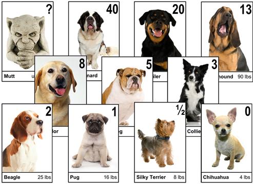
Figure 7.3 Typical card deck for agile “estimating poker.”
Note that the deck does not include every number between the two extremes. Agile developers do not like to lose time debating whether a particular story is a 6 or a 7. By spreading the numbers out a bit, card decks make group decisions easier and keep the process speedy without losing too much accuracy. The typical agile estimating deck employs an expanding series of numbers. The most popular pattern is the Fibonacci series, which starts with 0 and 1, and then assigns to each succeeding card the sum of the numbers on the prior two cards. By convention, agile teams employ this series up to 13 and then switch to rounder numbers such as 20, 40, and 80 beyond that. Typical decks also include a card with a question mark (the “mutt” in Figure 7.3) so that a developer can signal he does not believe the team has enough information to provide an accurate estimate.
The process for using these cards to make an estimate proceeds as follows:
1. Have the product owner and other team leads present the story.
2. Each developer selects an estimating card expressing the size of the work required by the story.
3. All developers show their cards at once.
4. The scrum master identifies the highest and lowest individual estimates and asks those developers to discuss their outlying values.
5. Teams reselect and display estimating cards, discussing outliers and reestimating until a consensus is reached.
Before the estimating session begins, the team must identify or review its reference stories. As described earlier in Chapter 2, these stories pertain to a few work units already completed that the developers know quite well. The team only needs a couple of these reference stories, ranging from small to fairly large. The team gives the smallest of these stories an arbitrary number on the low end of the number line, such as a two or a three. The team then awards points to the other reference stories that reflect how much more work they represent compared to the smallest unit. Say a team has picked three such stories to serve as their references and assigned them three, five, and eight story points. The developers do not obsess about how many hours went into each module built, but they are very clear in their minds that the module built for the five-point story was nearly twice as much work as the three and that the eight was nearly three times as large.
To estimate a story from the top of the project backlog, the team discusses the requirements with the product owner and then considers briefly the technical work it will entail. As they talk, they should be striving to pick a card that best represents the size of the new story compared to the reference stories. The scrum master watches the developers during the discussion, and when it seems they all have a card selected, he asks them to “vote” by showing their cards.
Even in established teams, these votes will not match at first, but they often cluster closely around a particular value. At that point the team needs to discuss and revote until the estimates converge upon a single value. What if a team of nine developers voted a particular story with one 2, seven 8 s, and a 20? Instead of going with the majority, the scrum master immediately polls those with the outlier estimates, asking “What do you see about this story that the rest of us have overlooked?” In a typical data integration estimating session, the developer voting 20 might say something like “To build this customer dimension, we’ll have to deduplicate the account records from three different sources. We’ve just upgraded the data quality engine, and the new version is a nightmare. The labor it will take to deduplicate our account records now is going to kill us.” This comment will undoubtedly spook the other developers, who will frantically start searching their decks for the 20-point cards. But the scrum master should turn to the developer voting 1 story point and ask “What do you know that the rest of us don’t?” This developer might reply with “The data quality engine may now be a nightmare, but the accounts receivable team just put a new service online that returns a golden customer record. All we have to do is send an account list to the right Web address and it will send back a set of standard customer IDs.” Convinced by this suggestion, the other developers will search instead for their 1-point cards so they can revote the story.
In the estimating poker technique, as long as teammates disagree over labor-hour requirements, the scrum master asks them to place additional evidence and analysis before the team so that the disparity can be resolved objectively. The emphasis on outlying votes and objective resolution works to avoid group think, ensuring that important information is not overlooked and that no one person dominates the process. Although several iterations of voting may be needed before the team reaches consensus on a story, the time involved is mostly dedicated to analyzing the situation. The actual process of polling the team for an estimating process does not take very long, typically between 3 and 5 minutes per story. The poker technique can move at this quick pace because it is using pair-wise comparisons between the unestimated work and the reference stories. This is an intuitive process that draws upon the best parts of the human mind. The waterfall alternative is to break work down into microscopic tasks and estimate the labor hours for each—an excruciatingly detailed endeavor that quickly exhausts even the best software developers.
Because agile estimating is fast and easy, teams can achieve remarkable consistency and accuracy with their agile story point estimates. With estimating poker, agile estimating sessions stay fun and retain the attention of all developers, for they know that the estimates they provide will directly determine whether they work nights and weekends during the coming sprint. Although it is fast and easy, the estimating poker “game” is not an undisciplined approach. It is actually a lightweight version of the “wide-band Delphi” estimating technique, which has considerable research vouching for its effectiveness. [McConnell 2006]
Occasionally, teammates will split into two irreconcilable groups on a particular story, one voting 8, say, and the other voting 13. If the discussion is no longer revealing any new information addressing the disparity, then the scrum master can propose they just split the difference, call it an 11, and move on. Two story points one way or another should not make or break a sprint. If the team frequently divides into such implacable groups over estimates, then the scrum master should inquire as to the root cause during the next retrospective. A frequent divide within the group can represent a deeper division, such as two incompatible architectural preferences (such as Inmon versus Kimball) or the fact that the project involves two completely different types of work (such as dashboarding versus data integration) that might be better pursued by two separate teams.
A high point estimate for a story—say a 40—can indicate to the developers that they are discussing not a story, but a theme or an epic. This outcome should spur the scrum master into having them discuss how to break the story into smaller deliverables. Once teams get established, they often develop a “resonant frequency” with the estimates for their backlog stories. The bulk of their stories fall within a range of three consecutive cards, say 3, 5, and 8. This tendency reflects a dynamic scrum masters should encourage because it means the product owner and project architect are looking past epics and themes and bringing consistently defined user and developer stories to the story conferences. Such consistency is welcomed because it will allow the developers to optimize their development process for these standard-sized stories. They will achieve maximum velocity by sticking to common story sizes, keeping out of the backlog the oversized stories that will only “gum up” their DWBI application delivery machine.
Story points and ideal time
As discussed in Chapter 2, because Scrum/XP is really a collaboration model and not a complete method, there is tremendous diversity between agile teams. When it comes to estimating, the most fundamental variation observed is whether a team employs story points in addition to labor hours, as outlined in this book, or skips story points entirely to estimate work only in labor hours. The latter style is called the “ideal time” approach. Because ideal time estimation certainly works for many teams, one would be hard pressed to say its advocates are committing an error. However, there are several reasons to think that employing story point and labor hours performs better. A list of the pros and cons for each approach will allow readers to decide for themselves which choice is right for their teams.
Table 7.3 sets forth the major poles defining the diversity in estimating styles. Other variations exist, but they become readily intelligible once one understands the differences portrayed here. The primary contrast is depicted in columns 1 and 2, that is, between the two approaches taken by generic agile teams: story points or ideal time. For clarity, the table also lists in columns 3 and 4 the approaches recommended in this book for agile data warehousing, where the variation is driven by whether a team is pursuing mostly front-end, dashboarding work or back-end, data integration work using data.
Table 7.3 Summary of Contrasting Agile Estimating Approaches
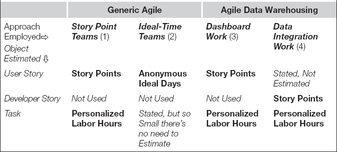
Column 1 in Table 7.3 depicts the generic story point agile team as estimating user stories in story points and then tasks in labor hours. Column 2 shows that an ideal-time team estimates user stories in work days for an anonymous developer operating under ideal conditions. The ideal-time team estimates in “anonymous” labor time, whereas the other three approaches use personalized labor hours at the task level, a point discussed in more detail in a moment. Often ideal-time teams will only enumerate the tasks within each iteration, keeping them so granular (2 to 4 hours) that the team need not waste any time estimating them. They believe it is more efficient to simply work those tasks and get them done. Because both columns 1 and 2 portray generic agile teams building OLTP applications, neither of them need to concern themselves with developer stories.
Columns 3 and 4 of Table 7.3 depict our recommended approach for agile data warehousing. If the developers are pursuing front-end, BI stories only, their work is very much like that of OLTP projects. Although the work will entail mostly user-interface elements that must be moved about the screen and enriched as the product owner requires, the team can deliver user-appreciable results with every iteration. These teams can safely pursue the project with just user stories estimated in story points and tasks estimated in hours. For data integration projects, however, teams will not be able to regularly deliver results that end users can work with or value. These teams will find their work much easier to understand and estimate if they utilize the developer story decomposition scheme suggested in the previous chapter. For data integration stories, then, teams award story points to developer stories rather than user stories. For development tasks, they will still estimate in labor hours as done for dashboarding work.
Story points defined
With the contrasting styles of story point and ideal-time estimation now outlined, readers will benefit from a more careful definition of the two fundamentally different units of measure they employ. As described earlier, story points are a measure of magnitude or size of the work a story implies. Divining the labor implied by a particular story is analogous to guessing the weight of a piece of fruit, be it a cherry or an orange. One cannot specify exactly the object’s mass through simple visual inspection, but by knowing that an orange is half a pound and a watermelon is five, he can come reasonably close to predicting the weight of a cantaloupe. On a data warehousing project, developers may decide that a slowly changing dimension is an eight given that they have agreed that a simple transaction fact table load module is a two. Such a statement is analogous to saying that a cantaloupe weighs about the same as four oranges. Moreover, when a team decides that two eight-point stories will “fit” within a 2-week iteration, it is on par with saying that two cantaloupes and four oranges will fit within a 10-pound sack.
When teammates really press for a more scientific definition of story points, scrum masters can always suggest that a story point is simply a percentage of a team’s bandwidth, that is, its ability to deliver new application functions within one sprint time box. If the developers are currently delivering 20 story points every iteration, then 1 story point is 5% of that capability.
Ideal time defined
When teams estimate stories in labor hours, they will state that something as unalarming as “Story 126 will take 45 hours,” but it is important to remember that they are speaking in terms of “ideal time.” Ideal-time estimates are labor forecasts based on the assumption that whoever ends up developing the deliverables for a story will work only on that story until it is finished, and work under ideal conditions. There will be no interruptions or time drained away by departmental meetings, emergency emails, or idle chatter with one’s teammates. Ideal-time estimates also assume that working conditions will be perfect—every tool and datum needed to build the code will be readily available, and every piece of information needed to guide the coding will be supplied without delay. That these conditions will actually occur is highly suspect. Perhaps even more dubious is the fact that ideal-time teams estimate these work durations not for any one teammate in particular, but instead for an anonymous developer. By defining the labor forecasts for an ideal programmer in an ideal situation, developers can continue using a single team velocity for setting sprint goals rather than having to track velocity for each role on the team. [Cohn 2005]
The advantage of story points
As long as a team can reliably forecast a backlog’s labor requirements without investing too much time, the choice between the story point and the ideal-time approach will not matter. However, research and experience suggest that most teams will perform better using the story point approach.
The primary advantage of ideal-time estimates is that they are in hours. Hours are easier to explain to stakeholders outside the team, including project sponsors, the project management office, and team members’ function managers. No one outside an agile project understands “story points.” In fact, teams using story points cannot tell you the precise unit of measure they represent, and one team’s story points certainly do not match that of the next agile team.
The problems with ideal-time estimates appear immediately, however, and many of them are implicit in the definition of “ideal.” Ideal-time estimators forecast labor for an anonymous developer. During the estimating process, however, one developer might state that an ideal programmer can complete a story in 2 days whereas another insists it will take 4 days. To resolve the issue, they will have to identify a particular person to use as an example of programming style so that the notion of an anonymous programmer suddenly disappears. Now that they are discussing particular individuals on the team, they should start tracking the velocities for each teammate in order to avoid overcommitting during each sprint. More importantly, by pegging estimates to the precise programmer they think will do the work, they have instilled a tremendous constraint on the iteration. Programmers cannot share or exchange stories during development, else they will undermine the estimates and risk working nights and weekends in order to deliver new features as promised. Ideal-time estimation thus discards the advantages and speed achieved through a spontaneously self-organized team.
Research has shown that the human mind excels at comparing the relative size of two complex objects, but does poorly at identifying absolute magnitudes if there are more than a few abstract factors involved. [Miranda 2000; Hihn, Jairus, & Lum 2002] Ideal-time estimates consist of the absolute magnitudes that humans struggle with. It is possible for developers to estimate labor hours reasonably well for a small number of tasks, such as those making up a single iteration. Estimating more items than that, however, causes their minds to tire and the accuracy of their estimates to fall. Story point estimation requires the pair-wise comparisons research shows humans are good at performing. Being easy to generate, story points then make a far better choice for estimating an entire release or project.
Ideal-time estimation also suffers in the area of resolving disputes. When two developers provide wildly divergent forecast for the same work item, they are tempted to discuss the actions they believe each task will take. Discussions regarding step-by-step actions are far too granular. Such detail will slow estimating to a crawl, preventing the team from getting through a story conference quickly, not to mention a whole project estimating session. When the estimating effort required for individual work elements goes up, it saps the energy of a team working a long list of items, driving overall forecasting accuracy down.
Contrast these lamentable aspects of ideal-time estimates to the advantages of story points and the choice should become clear. Story points equal not hours but a more intuitive notion of a story’s size, such as its “weight” or “mass.” The hours the work requires are implicit in the size, so teams can work at this higher unit of measure and skip all the disagreements over detailed technical tasks and their proper durations. The developer who will pursue a work unit is not implicit in that module’s size, so the developers are free to swap roles during the sprint and share the load as necessary in order to get the job done in the shortest possible time.
The size of a story is also independent of the nature of the team. Ideal-time hours can shrink as a team gains experience with the problem space of the project or can grow when external factors make work more difficult in general, such as when developers begin using a new tool or a personal matter impacts the effectiveness of a key member of the team. With story points, such vicissitudes simply make the velocity rise or fall. The estimating units themselves do not vary, making story point forecasting much simpler for developers to keep consistent over the life of the project. Perhaps more importantly, the invariability of a size-based estimate allows a team to forecast an entire project and avoid revisiting that forecast constantly because the unit of measure has changed.
Story points can also tap an important second estimate that validates the programmers’ forecasting skills and quickly makes their estimating more accurate. Story pointing teams set the points for their work during the story conference and then corroborate them with the labor-hour totals assigned to component tasks during the task planning portion of the sprint planning day. Teams typically bounce back and forth during the planning day between story points and tasks hours until they get them both right. Ideal-time teams estimate immediately in hours, leaving them no other unit of measure with which to verify their projections. Without a double check, spurious factors can warp their estimates unimpeded and undermine their forecasting accuracy.
Crucially, story points do not mislead project stakeholders into misinterpreting the team’s estimates. When a team states a project will require 1000 ideal hours, the rest of the world hears only “1000 hours” and decides quickly that four developers should be able to deliver the whole application in less than 2 months. When a project is estimated in story points, stakeholders must ask what the team’s velocity is before they can infer a delivery date. This links everyone to the reality of the team’s performance and insulates the developers greatly from other parties’ tendencies to build unrealistic expectations. Story points also do not invite management overrides. When developers decide that a particular story will take 60 hours, project managers and functional supervisors can easily double guess the estimate, claiming that a “reasonably competent” programmer should be able to get it done in half that time. Story point estimates must be interpreted using the team’s velocity, thus again forcing everyone to utilize the historical facts that actual project experience provides, avoiding distortions caused by wishful thinking.
Finally, story points are just plain easier to work with. By avoiding issues such as who will actually do the work and how fast they should really code, teams can estimate each story in a few minutes once they understand the functionality desired. This enables them to keep story conferences brief and efficient, making it much easier to keep everyone involved. The ease of story pointing also makes it reasonable to estimate an entire project, allowing teams to provide regular forecasts of remaining work that sponsors demand from projects as lengthy as data warehousing efforts. Moreover, with ideal-time estimating, the team loses the accuracy and speed needed to regularly provide current estimates for the project. Without story points, it is difficult to provide the team’s prediction of how long a project will take, allowing stakeholders to develop contrary notions, which often result in developers having to finish the project under an extreme time pressure to meet an arbitrary deadline.
Estimation accuracy as an indicator of team performance
Team estimates provide a handy summary level measure for assessing the effectiveness of an agile team. When teams are executing their agile method effectively, they should be able to reliably deliver 95% of the work they take on with each iteration. To achieve this high level of performance, they must do everything right. They first understand the features requested, decompose them into properly sized stories, plan their delivery, collaborate well with each other, validate their work as they go, and provide working software so robust the product owner can evaluate the results using his own business questions to guide him. If the team fails to execute well on any portion of this chain, the ratio of accepted results to amount of work promised at the start of the sprint will take a rapid dive. Fast delivery of quality applications may be a primary goal for agile teams, but the accuracy of their estimates is the “canary in the coal mine” indicating whether something has deteriorated with the process in the project room.
The ratio of accepted-to-promised work can be calculated for every iteration in story points and labor hours. The possibility of two different units of measure adds some subtlety to working with this metric. The ratio for story points is simply the story points of accepted stories divided by the story points of stories promised at the start of the iteration. The ratio for labor hours is the total of labor hours on tasks that were completed—according to the team’s definition of done—divided by the total hours for all tasks associated with the promised stories. If the team delivers upon 95% or more of both story points and labor hours, they can be assured they are performing well. The ratio for story points can fall dramatically if even one story gets rejected. When this happens, the team must consider the ratio for labor hours. If the labor-hour ratio is also below the 95% mark, then it indicates that the team had trouble somewhere in its process and did not get all its work done. The drop in the story point ratio may be simply due to the amount of task work not completed. If the ratio for labor hours is above the 95% level, then the story must have been rejected for quality reasons, and the team should focus on that aspect of their process rather than on whether all the work was completed. The sprint retrospective is the natural forum for determining the root cause when either of these ratios falls, and exploring their movements often reveals the rough edges in the team’s development process.
Value pointing user stories
As described earlier, story points provide a sense of how much labor a given developer story for a data integration project will likely require. In that light, story points reflect a notion of cost, to wit the programming resources the organization will have to invest to acquire the capabilities described. Any estimate of cost naturally gives rise to a complementary question: how much will a particular unit of work be worth once completed? That is, how much will its promised functionality be valued?
Many agile teams use the estimating poker technique to derive not only story points but also “value points” for the components on the project backlog. Instead of obtaining those value points from the programmers, the team leads will hold a value-estimating session for the product owner and the project’s major stakeholders. Whereas it may seem natural for the stakeholders to award value points to the user stories, sometimes they are too granular. In that case the business partners will only be able to value point themes. They might ask “What’s the value of slicing revenue by customer? I can’t tell you. But understanding where we’re losing revenue, that’s worth twice as much as being able to review our costs.” If the stakeholders can only value point the themes, then the team can ask the product owner to finish the job and distribute them across the component user stories. As a default, he can award value points proportionate to the story points the developers set if no other way to proportion the value suggests itself.
The payoff of value pointing a project’s themes or user stories is severalfold. The result gives the team, including the product owner, a set of numbers they can utilize to place the user stories in priority order. Value points provide a notion of business benefit to consider when it comes time to rescope the project or contingencies require the developers to delay the delivery of a particular feature. The team can also prepare what the agile community calls a “burn-up chart,” a chart of benefits delivered by the project over time using the value points of the stories delivered against time.
If the project has been assessed a return-on-investment (ROI) measure, the value points contained in each major component can lead to a dollar measure of benefit by simply distributing the ROI across stories in proportion to the value points assigned to each. This practice will make the project burn-up chart of value delivered to date all that more compelling by putting it in dollars, a unit of measure that everyone can understand. A dollar-based graph of value delivered to date will allow the product owner to quantify the benefits of the project to sponsors whenever the project’s future funding is discussed. Value points translated to ROI dollars even allow the contribution of several projects within a program to be aggregated.
Finally, when the slope of the burn up from one project begins to level off, the program can consider whether the company would be better off transferring those resources to another project. Thus value pointing enables companies to allocate their programming resources far more effectively, making them well worth the small amount of time they take to gather. The burn-up chart will be considered again in the last chapter of this book.
Packaging stories into iterations and project plans
An earlier discussion in this chapter mentioned that some agile teams will refuse to provide their stakeholders whole project estimates. Unfortunately, the length and high expense of data warehousing projects invariably require a labor forecast if the project is to be funded. Sponsors may provide a little “discovery” money to get started, but soon the executives will require a cost target and a calendar goal for the project. Data warehousing stakeholders commonly insist upon such estimates so that they can judge as the project progresses whether a team is performing and whether the scope of the project is under control. The product owner, under heat from the sponsors, will also demand a schedule of iterations listing the features that will be achieved with each sprint. These demands require that agile warehousing teams learn to bundle user and developer stories from the backlog into attractive releases, where each provides valuable new services to the business departments of their company.
Fortunately, a project backlog with story point estimates provides the raw material for preparing these major artifacts. They require only that the story points have been estimated and a measure of the team’s velocity. Both the story estimates and the velocity must be in story points. To derive an estimate for a whole project or for just the release ahead, the team must group the stories in the backlog into iteration-sized chunks. Figure 7.4 shows the end result of this process for a data integration project, where the backlog’s detailed lines represent developer stories.
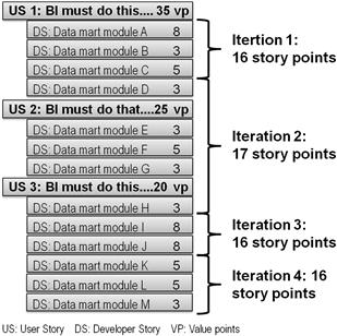
Figure 7.4 Deriving a current estimate from a project backlog.
In Figure 7.4, user stories are shown as headers over the related developer stories. They have been “appraised” by the stakeholder community using the “value points” in order to facilitate their prioritization. Story points are visible on each developer story, and they are what the team has used to group stories into iterations, using in this case a velocity of 16 story points, which they must have achieved during the prior iteration. At this point, developers can communicate to stakeholders that the entire deliverable represented in Figure 7.4 will require four sprints. If they are using a 3-week time box, simple math allows them to state that four sprints will take them 12 weeks. To derive a cost projection for the sponsors, the team can simply multiply its per-iteration burn rate by the number of necessary sprints that the bracketing process has indicated. If, in our example, the project is consuming $100 K per iteration, simple math again reveals that the team will need $400 K to deliver all the modules listed on the current project backlog. By this means, agile teams can provide stakeholders an answer to “how long is it going to take and how much is it going to cost?”
As each iteration concludes, the team will acquire a new measure for its velocity. To prepare a current estimate of the cost and duration for the remaining development work, the team needs only to bracket the remaining stories on the backlog using their existing story points and the new velocity. This step will provide an updated count of the necessary iterations, which in turn will indicate a new forecast for the remaining development cost. Occasionally, teams will realize that they misestimated an entire class of stories and need to adjust their story points. For example, a data integration team might decide that all slowly changing dimensions need to contain the previous value for certain fields on the current record rather than just tracking history with inactive records, that is, they should be Type 6 rather than Type 2 dimensions. This decision will increase the typical story point for many of the project’s developer stories involving slowly changing dimensions, say from a five to an eight. Such an adjustment is again easy to include in a new current estimate by simply revising the story points for that class of stories and rebracketing the backlog using current team velocity. Agile’s current estimates, based on story points and team velocity, are quick to create and update, plus they are readily understandable by all stakeholders.
Criteria for better story prioritization
Bracketing a backlog’s stories using team velocity to derive a current estimate presupposes the team has placed the stories into the right sequence. In practice, teams usually alternate a bit between sequencing and bracketing in order to derive a delivery plan of iterations that all roughly match the team’s velocity. Additional factors also come into play as the team discusses ordering of the stories. All told, there are six considerations for sequencing the stories of a backlog, as listed in Table 7.4.
Table 7.4 Six Steps for Prioritizing Project Backlogs
Agile has only one priority: Business Value
Teams can Lower Risks by Considering Additional Criteria:
1. Predecessor/Successor Dependencies
2. Smooth out Iterations
3. “Funding Waypoints” in Case Resources Disappear
4. Architectural Uncertainties
5. Resource Scheduling
Generic agile recommends that the product owner sequence the stories according to business value, and certainly this is the place to start. By sequencing in business priority, the team will ensure that it delivers the maximum value possible should the project get canceled before it is completed. However, if members of an agile warehousing team did not look beyond simple business priority, they would be risking several other factors that could easily make the project fail. Table 7.4 lists five prioritization criteria beyond the simple business value necessary to mitigate these risks. The next consideration should be ordering the stories to account for data and technical dependencies. For example, the product owner may insist upon slating the “load revenue fact table” developer story at the top of the backlog, so the team will need to gently assert that at least some of the dimensions need to be delivered before loading a fact table makes any sense.
The third consideration on the full list of prioritization criteria would be to swap developer stories in and out of iterations in order to “smooth” each bracket down to match the team’s velocity. If the team has a velocity of 15 story points, it makes no sense to have a sequence that requires 12 points in one iteration and 18 in the next. A better solution would be to swap a 5-point with an 8-point story so that both iterations match the team’s velocity of 15. Naturally, the product owner needs to be included in these discussions, but unless the team is starting the last iteration before a release, such “horse trading” between iterations will have no impact on the stakeholders the product owner represents.
The next sequencing criterion focuses on “funding waypoints,” which are the places within a project plan where the organization might reconsider whether to continue funding the development of the application. This criterion asks the product owner to consider the value of the project, assuming it is not funding past each release boundary. This consideration can lead him to spot a user story far down on the list that the business cannot live without, even though it made sense somehow to develop it later in the project. The story could be a tool supporting annual reconciliations between warehouse data and operational systems. The product owner did not feel he must receive it right away, but he knows the company will need that feature eventually if the product is going to be complete. When faced with funding waypoints that might cause the bottom of the list to be dropped, such stories should be moved up before the release boundary in question in order to minimize the impact of a possible project cancellation.
At this point, the stories are in a logical order and reflect the highest possible value to the business. The project architect should now search for the technically riskiest stories on the backlog and consider elevating them to earlier iterations. Take, for example, a profit margin data mart project in which the product owner has placed the revenue fact table at the top of the backlog. The project architect might realize that the transformation for the cost fact table will require a standard costing subprocedure and have serious doubts whether data available are complete enough to power the algorithm everyone has in mind. Accordingly, he should advise the product owner to elevate the story for the cost fact table above that for revenue facts so that the team can build enough of the allocation engine to prove the technical feasibility of the entire project.
Finally, resource availability can often impact the optimal ordering of a project backlog. Say the product owner has organized the backlog to steadily deliver a series of dashboards with each iteration, but the BI developers will not be released from another project for another 4 months. Here it would make far more sense for the team to build all of the dimensions before the fact table behind even the first dashboard, because without a BI front end there is no compelling reason to rush the fact tables into production before all their dimensions are ready.
Segmenting projects into business-valued releases
The criteria presented previously work well for ordering a project backlog, but ordering alone does not provide a full project release plan. To get the necessary feedback on requirements and to maintain project funding, agile teams must regularly push new capabilities for end users into a production environment. For this purpose, good sequencing is not enough. To plan out a steady flow of valuable features for end users, the team will need to devise ways to package the project’s stories into a series of functional enhancements for the application that end users value. “Project segmentation” is the practice of selecting points along a project backlog where an intermediate version of the software can be placed into production for end users to benefit from. Effective project segmentation balances sequencing stories in order to avoid rework for developers against bringing forward certain features that will please the end users and project sponsors. Project segmentation first occurs at the end of the project’s inception phase as part of deriving the whole project vision and cost estimate required by the project funding process of many companies. Once the project’s construction phase begins, teams frequently revisit project segmentation whenever business or technical needs change in order to redefine the sequence in which features will be delivered.
Segmenting a project defines a series of production releases where each provides a compelling stakeholder benefit. However, incremental delivery means all but the last release will be missing some features, so any proposed release schedule will mix benefits with frustrations for users. Negotiating an acceptable series of releases can be very difficult when working with a stakeholder community that wants all data, wants it perfect, and wants it now. There also may be certain milestones a project must achieve to coordinate with other IT projects in the company. The team must find a set of natural dividing lines within the stakeholder’s notion of “the data warehouse” along which reasonable, partial deliverables can be defined.
While planning their project segmentation, agile data integration teams usually cycle through three steps utilizing three artifacts: dividing up the project’s star schema, finding corresponding divisions on the project’s tiered integration data model, and summarizing project releases using a categorized services model. To keep the presentation of this process clear, the following text first recaps the data engineering solution engineering approach by which teams derive the data models employed, then describes three artifacts employed, and finally illustrates how they are used to segment the project into an incremental series of application releases.
The data architectural process supporting project segmentation
Because project segmentation determines customer satisfaction directly, it is a primary practice needed to make agile data warehousing projects succeed. Conceptually, it occurs at the end of a long chain of activities pursued by the data architect with wide support from the other teammates. In waterfall methods, these activities follow a precise sequence, as prescribed by enterprise architectural planning and standard system engineering. On an agile team, the data architect iterates between them while reviewing the results with the rest of his team, providing greater detail with each pass. Typically, agile teams work an architectural plan until the artifacts cover the most important 80% of the project. In the interest of getting the project started and to begin learning from actual results, the team considers these 80/20 specifications “good enough” and leaves the remaining details to be specified when the developers begin building modules during an iteration. Although agile teams move between engineering steps as needed to achieve a workable design, it helps to know the logical sequence these steps should occur in helps understand project segmentation. That ordering can be summarized as follows:
• Business modeling in order to identify required informational entities and to resolve any conflicts in terminology and semantics through data governance. In agile projects, authoring user stories that describe the desired application is included in this step.
• Logical data modeling in order to represent the data entities and attributes indicated by business requirements, but to depict them independently of how they will be implemented in the physical tables of the database. In agile projects, decomposing user stories into developer stories occurs during this step.
• Physical data modeling in order to specify the precise tables, views, indexes, constraints, and other database elements the team will need to create and populate in order to deliver the services depicted in the logical and business models.
Artifacts employed for project segmentation
In an agile data warehousing project, the data engineering steps listed earlier result in a set of artifacts that assist greatly in project segmentation. For data integration projects, project segmentation must be preceded by a good start on developer story decomposition, story point estimating, and whole project planning, as presented in the past few chapters. In addition to a prioritized and story pointed project backlog, segmentation requires a few additional artifacts to enable the team—including the product owner—to fully envision various alternatives and reasons about the advantages of each. These artifacts are as follows.
Business target model
The business target model is a business-oriented presentation of the application’s dimensional model. It depicts major business entities as a set of facts and dimensions the customer will need for his data mart. The team uses this model to understand the purpose of the data warehouse it is building for the end users. This artifact was first introduced in Chapter 5, and Figure 5.4 provided a good example of such a model. As in that diagram, the business target model is often drawn schematically, with only the entities identified, or at most a few key attributes. Because the objective of dimensional modeling is to provide business-intelligible data stores, often a data mart’s subsequent logical data model closely resembles the relevant portions of the business target model.
Dimensional model
The dimensional model is a logical data model of a DWBI application’s presentation layer (introduced in Chapter 6) from which the end-users’ dashboards will draw data. It lists the entities and attributes the envisioned dashboards will require. Those entities providing measures are called facts. Those providing qualifiers by which facts can be disaggregated, filtered, and ordered are called dimensions. The top half of Figure 7.5 provides an example of a dimensional model. Typically, facts appear central in these models with dimensions surrounding them. Again, because dimensional modeling strives to make presentation layers intelligible for business users, dimension models appear very much like business target models, only with more details regarding the attributes of the entities. In the figures discussed later, dimensional models are depicted schematically (entity names without many attributes specified), which is often the way agile warehousing teams will draw them while planning projects on team room whiteboards.
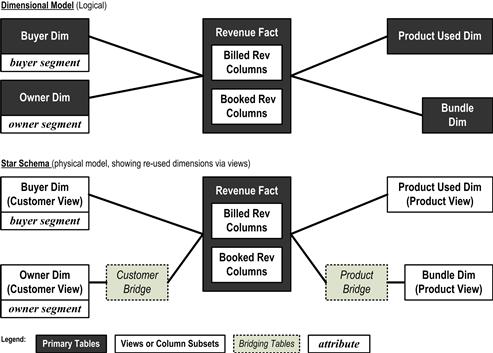
Figure 7.5 Sample dimensional model and corresponding star schema.
Star schema
A star schema is a physical model of the database tables needed to instantiate the logical dimensional model discussed earlier. The bottom half of Figure 7.5 provides a schematic depiction of the star schema employed by the examples in this chapter. Star schemas can often appear very much like their corresponding dimensional models occurring upstream in the definition process and also very much like the business target models that occur upstream from that. However, as can be discerned in Figure 7.5, the physical star schema can provide additional information covering the substitution of views for physical tables and the role of “bridging tables,” both of which are discussed during the example given here.
Tiered integration model
The tiered integration model is a physical model of the integration layer. It differs from a standard physical model in that (a) its tables are often depicted schematically with all table names, but attributes only where necessary, and (b) tables are arranged in levels that reflect the number of parents each has so that the team can identify dependencies between them easily. Figure 7.6 depicts tiered data used in this chapter’s examples.
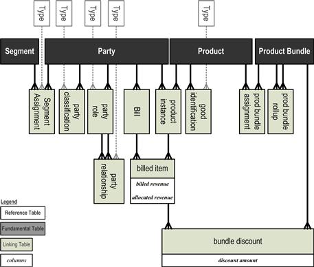
Figure 7.6 Sample tiered data model for an integration layer (drawn schematically).
Categorized service model
A categorized services model is a diagram that identifies a few important categories of service for end users that the development team can add to the application in increments. This model also displays major steps along each of those categories that define intermediate levels in the richness of service provided, allowing teams to select which level to include with a given release. Figure 7.7 depicts a categorized services model for the front-end “domain” of dashboard components for a data warehousing project. Figure 7.8 presents a similar model for the back-end domain of data integration work that many business intelligence projects also require.
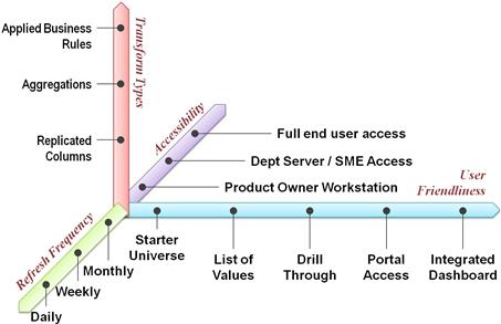
Figure 7.7 Front-end project categorized service model.
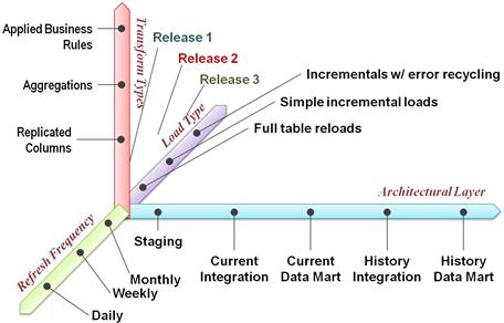
Figure 7.8 Back-end project categorized service model.
Each of the sample diagrams has divided the services of its particular domain into four categories. It is important to realize immediately that every team will probably select a different number and set of categories for its service models. In the examples provided in these figures, the front-end model uses for its categories the “user-friendliness” of the dashboard, the access user will have, transformations embedded in the front end, and the frequency with which the BI tool will refresh its data subsets from the presentation layer. The back-end model defines its first two categories using the layer from the project’s macro data architecture (discussed in the previous chapter) and the style in which it refreshes the tables in those layers with new data from the operational layer. The other two categories match that of the front-end model.
Each category provides its own collection of progressive service increments. These increments will be used to define the intermediate waypoints within the categories that the team can use to define a series of incrementally better product releases. The front-end category for user-friendliness, for example, defines a series of waypoints that progress along four levels of service, including (a) simple models for the semantic layer, (b) a list of values for query definition screens, (c) the capability to “drill through” a display to listings of data values behind a dashboard element, and (d) an integrated interface including may dashboard elements in a single compact display. Just as each team may define its services model with different categories, each project’s developers will also pick the set of service waypoints on those categories that best address the project they are working on.
The earlier discussion identified the general data engineering process teams should follow and identified several artifacts to employ. These two elements will allow an agile team to negotiate major project releases with its stakeholders so that the overall project plan is not only reasonable from the developers’ point of view, but also follows a path providing the highest end-user business value possible.
Project segmentation technique 1: dividing the star schema
To recap the choices available for negotiating with stakeholders a project’s major releases, the team can segment the project by (a) dividing up the project’s star schema, (b) finding corresponding divisions on the project’s tiered data model, and (c) summarizing project release using a categorized services model. The first of these approaches is fairly simple minded. Segmentation by dividing up the star schema occurs when the team draws the project’s star schema on a whiteboard and begins drafting lines around the tables to define a series of project releases.
In truth, drawing lines on the star schema is only the last step in a process that roughly follows the steps enterprise architectural planning listed earlier. We continue with the example employed during the prior two chapters to illustrate how a hypothetical agile team arrived at a particular project segmentation plan. The sample team’s goal is to identify a set of incremental releases that have value for the business. Therefore, the first step was to focus on user stories most important to the product owner. From Chapter 5, the top user story was worded to be “As a corporate strategy analyst, I need a dashboard of monthly billings with full customer demographics and product details…for business marketing group’s eastern region…allowing analysis of customers subscribing to each service so that we can better design promotions by product type.” The product owner also paraphrased this story as “Who is subscribing to what services, as seen through monthly billings?”
With the driving user story identified, the team then considered the dimensional requirements from all three architectural viewpoints, progressing from the business target model to the application’s logical dimensional model and then to the physical star model. Because dimensional modeling had caused these closely resembling each other, it was easy for the team to simultaneously draw the same candidate segmentation lines on all three. Figure 7.9 shows how the final set of candidate lines appeared on the physical star schema. Note that most table column and several dimensions, including date, have been omitted for clarity.
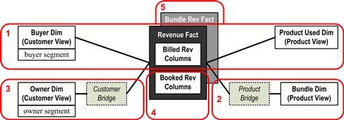
Figure 7.9 Project segmentation lines drawn on a star schema.
The dialog that led to the lines displayed in Figure 7.9 unfolded as indicated in the following transcript, stylized to keep the presentation short.
Paula, project architect: Okay Carla. You’re our product owner so I’ve got to tell you that the full data mart the business has requested cannot be delivered in one iteration or even in one release if we want to put something into production every couple of months or so. Your highest priority user story focused on “Who’s buying what?” Consider the group of objects I’ve identified with Circle 1 on our set of dimensional models. You can look at the business target model, and the rest of the team will be looking at the physical star schema, as the circle is approximately the same on each. Circle 1 says we will push a build onto the production server that will allow your users to analyze billed revenue columns by the party that bought a service and the product that they are using.
Carla, product owner from corporate strategy: Will the first release allow me to see the market segment the customer belongs to?
Dale, team’s data architect: Yes, but only the segment of the buying company. We know you have a business rule requiring that the segment of a buying company should be overridden by the segment of their owners if the owners are considered a “global account.” You won’t have any information on owners if we segment this project according to Circle 1.
Carla: How about product bundling? Our customers buy packages of services and equipment called “bundles,” but the billing system charges them for the atomic components within those bundles, applying a discount later at the bill header level for the bundle.
Dale: We’ll be limited by Circle 1 on that aspect, too. With this first release, you’ll only be able to identify the charged products, not the product bundle the customer ordered.
Carla: And what about the allocation of billed revenue to monthly components for customers paying quarterly?
Dale: Circle 1 will only give you billed revenue, so the metrics your user will see will be a bit “lumpy.” According to our systems analyst who profiled data for the Easter business marketing group, omitting allocated revenue will affect about a quarter of the customers.
Carla: We can wait for the allocated revenue, and even revenue adjusted for bundle discounts, but I would really like to get owner segments, product bundles, and allocated revenue in the first release.
Paula: We’ve defined and estimated developer stories for all of those data elements. That collection of features is about 8 months of work. To stay agile, we’d like to have three incremental releases in that time frame, not just one, in order to provide some value for your end users as fast as possible. What if we drew Circle 1 so that it included everything on the left side of the diagram so you’d get buyer and owner segments in the first release? The product would not be part of the first set of dashboards.
Carla: No, owner segments are not as important to that user story as the actual product a customer’s using.
Paula: What about if we drew Circle 1 around everything on the right side so you got product used and the bundle it was sold in? Customer would not be part of that first release.
Carla: Bundles are more important than owner segment, but not more important than knowing who the buying customer is.
Dale: Then we hear that the first version of Circle 1 is the best collection of analytical capabilities we can give you as a first release at the 2-month time mark. We should then aim for providing product bundles next and then customer owners. After those are both delivered, we can work on the data transforms for allocated revenue. Let me draw Circles 2 through 3 on the model here…. You’ll notice on our physical star schema that I’ve included the bridging tables in those other circles. The one on the left allows us to do the rollups from buying company to a holding company, even if there’s several layers in between. [Kimball 1998] Likewise, the one on the right allows us to do the rollups for products into bundles. We’ll be using views so that in the long run we can provide buyers and owners from a single set of customer tables and products used and bundles from a single set of product tables. [Kimball 1997]
Paula: The story point estimates we made using this project’s developer tell us that with the team’s current velocity from its last project, we’ll be able to deliver each project segment circles in 2 months.
Dale: I’m drawing two more circles for releases we’ll deliver after that. Circle 4 involves business rules for allocating revenue, and Circle 5 will provide a second version for all revenue tables that includes the discounts for bundles.
Carla: So, I’m taking your word on how long each group on this diagram is going to take, but you’ve drawn those boundaries in the right order.
Paula: We’ll maintain a current estimate for you. If the team’s velocity improves, we’ll be able to recalculate and tell you how much earlier we can deliver.
Project segmentation technique 2: dividing the tiered integration model
With the negotiation just given, the team established an acceptable series of end-user features with the product owner. Unfortunately, this series is defined only in terms of the presentation layer of the project. When the project architect cited team estimates suggesting that each delivery group would require 2 months, she had to be taking into account the integration layer that the data architect has stipulated for this project. In our example, the team concluded its user-level negotiation with the product owner using the set of dimensional models and then convened an integration-layer segmentation workshop involving the project architect, data architect, and systems analyst. At this workshop, the team will concentrate upon the integration-layer segmentation needed to support the desired segmentation identified for the presentation layer. By drawing a corresponding series of candidate deliveries on the integration’s tiered data model, the team can decide quickly whether the implicit integration work of the negotiated schedule will be indeed reasonable for the programmers.
Figure 7.10 shows the project segmentation the team from our example drew upon the tiered, physical data model for its integration layer. The conversation was led by the data architect, as he authored the tiered integration model and could best link its components to the elements and groupings drawn on the star schema. A transcript of Dale’s comments while applying this second technique follows.
Circle 1 on the star schema requires us to have billed revenue, buying customers, and charge products. On the tiered integration model, billed revenue is found in the billed item table. The buying customer is found in the party table, and the charge product in product. To link these tables together so we get data needed for Circle 1 on the star schema tables, we’ll need everything in Circle A1 on the tiered data model. That won’t be enough for the first release, however. We must provide the segment for the buying customer, so we’ll have to have records from Circle A2 as well.
The second project segment we negotiated with the product owner was for product bundles, and that would be this Circle B that I’ve drawn on the tiered integration model. Likewise, owner market segments will require the tables included in Circle C on the diagram. I can see that the allocated revenue will be a second set of columns in the product instance billing table, whereas bundle discounts come from a bundle discount table. In both cases, we’re fortunate. Adding the features for Circle B, C, and beyond will not require us to include any new parent tables for bottom-level tables we already populated, so there will be minimal rework with this segmentation plan.
So now we can easily figure out the data transform modules we’ll have to build in order to get the required data loaded. Let’s see if the work defined for the three releases making up the first full version will doable given the time we have:
• We’ll have nine target tables comprising two reference tables, three fundamental tables, and four linking tables.
• I’ll have to model them in detail and get the DBA’s to create them in the target schemas.
• The systems analyst will have to specify any data transforms needed by any of the target columns.
• The programmers will have to build both initial and incremental load modules for all nine tables, which is approximately 18 modules.
• We need to reserve a good week for our tester to load full volume data and conduct the system tests before we can promote onto the near-product server for user acceptance testing.
Paula said two and a half months for all the developers’ stories in Circle 1. That’s 9 weeks after subtracting a week for system test, or three iterations with our 3-week time box. Nine weeks for coding 18 modules after all the 80/20 specifications are prepared. Judging from how things went on the project we just finished, it seems tight, but doable.
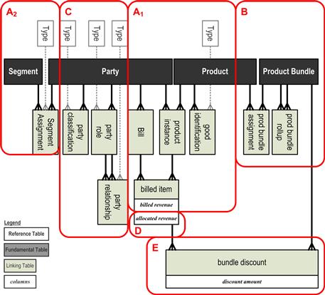
Figure 7.10 Project segmentation using a tiered integration data model.
The data analysts reasoning just described reveals several important aspects of performing this second segmentation step with the tiered integration model. First, the analysis occurs at a predominantly physical modeling level, but because the business and logical modeling preceded it, the team did not risk overlooking business semantics or logical requirements that would have invalidated the planning performed using the physical, tiered data model.
Second, much of the required information for this second step in project segmentation was prepared ahead of time and made possible by the developer story workshop described in the previous chapter. Because the data architect had been able to prepare a tiered data model based on the developer stories, it was ready when the team reapproached the product owner to negotiate project segmentation. Similarly, the story points that allowed the project architect and data architect to rapidly appraise the labor requirements for each circle had been derived earlier by working from the list of developer stories. Of course, as further discussions and analysis such as outlined in the aforementioned transcripts occur, the team may have to improve upon its collection of developer stories and/or their story point estimates. For the most part, however, project segmentation utilizes existing knowledge; therefore, developers can resegment quite responsively during conversations with the product owner.
Third, as the circles on Figure 7.10 reveal, tiered data models allow the team to define small vertical slices of the overall project that are deliverable independently. This pattern is the core to agile data warehousing, making it possible to identify and plan for incremental deliveries that entail a minimum of rework. If, contrary to our example, the data architect had found that elements in later releases required parents to be added to already loaded tables, then rework would be required. The degree of rework implied may have precluded a particular candidate segmentation plan, but in either case the tiered data model would have allowed the team to reason about whether the rework was worth the accelerated deliveries it would have supported.
Project segmentation technique 3: grouping waypoints on the categorized services model
Some qualities that teams can use to define project segments cannot be depicted on any data model. To segment a project using these qualities, a team must employ the categorized service models. The application qualities that these artifacts model frequently determine the level of service that end users will receive from a DWBI application, such as the frequency of loads, the volumes it contains, and the types of columns that have been populated with values. Figures 7.7 and 7.8 portrayed the notion of categorized services for both the front-end, dashboard service domain and the back-end, data integration service domain of a data warehousing application. The categories that defined each of these domains provide the team with a set of service waypoints with which a series of increasingly service-rich releases can be identified. The concentric rings in Figure 7.8 depict a series of releases for back-end services that the team in our hypothetical project negotiated with its product owner. Because such negotiation sessions sometimes touch upon the different types of columns that each release will have populated, the team’s data architect is usually included. But the full set of service decisions involved in these negotiations address how the various releases will represent solutions to the end-user’s business needs. Discussions at the solution level require the project architect, who usually leads these meetings. The dialog that established the releases identified on diagram in Figure 7.8 followed the following transcript.
Paula: Carla, there’s other categories of data mart features that we can compromise at first so that the developers can deliver some partially working systems very quickly. See if you can follow along on this services model diagram. Each of these categories provides several choices, and I need to find out from you which combinations of those choices would represent usable versions of the application for your users.
Carla: You mentioned this before concerning the back-end capabilities. Didn’t you suggest the team place only current data in the warehouse first and then later beef up the data transforms to place history records online as well?
Paula: Yes, that choice has to do with the “architectural layer” category in the diagram. We’re planning on using some views and our company’s “virtualization software” to split the current data into two deliveries. In the first release, we can populate only the integration layer and then create a virtual data mart of current data on top of that. That will provide your users some analytical capabilities. It will also give the developers time to build a full data mart of current data for the second release and then add in history records for the release after that. The compromise the virtualization tool will force on us for the first release is that your users can only submit queries that return a limited volume of data and don’t involve any advanced business rules.
Carla: Well, if we load just the eastern and central regions for the business marketing group, we should have only about a tenth of the full data, so big queries won’t be an issue. The limitation of basic business rules shouldn’t pinch too much, either, because at first we’ll be just performing counts and building lists as we get to know the data.
Paula: Okay, great. So that defines three steps concerning the project’s architectural layers. We’ll also want to take three steps along the “load type” category. We’ll start Release 1 with full table reloads—“kill and fill” loads—as long as we have small volumes because full reloads are easier to program. When we get to larger volumes, we’ll have to switch to scanning the sources for changed and new records, so Release 2 will have simple incremental loads of whatever has changed since the last ETL run. After that, we’ll add in some error recycling features for Release 3 so that you can see the source records that won’t load because of data quality issues occurring in the operational systems.
Carla: Didn’t you want to defer the complex business rules also?
Paula: Yes, that has to do with the “transform type” category. If okay with you we’d like to build Release 1 for just columns that get replicated as is from the source system. That would cover just billed revenue. For Release 2, we’ll populate the columns holding aggregations, such as Top 100 Customers. We’ll finish with Release 3, which will handle the complex business rules, such as allocated revenue and applied bundle discounts.
Carla: Well, the first set of user story is essentially “who’s buying what” in the business marketing regions. We can get close enough to an answer for that question on billed revenue alone. Allocated revenue address user stories were written for finance and regional executives, and they are pretty far down the project backlog, so it’s okay to defer those until the third release.
Paula: Super. The last type of service we’d like to deliver in steps is the frequency we refresh data in the data mart. Because we’ll be running the loads by hand at first, I like to give the first release just a load on the first of each month. We can get the load process mostly automated for Release 2, but it will still take some manual support for the reference tables. Given that, we’d like to move to only weekly for that release. By the time we get to the third release, we should have the kinks in the load routine worked out, making daily loads possible.
Carla: Daily loads are also of interest to finance only. The rest of us can live with weekly and even monthly at first while we’re getting to know the data.
The concentric lines on Figure 7.11 connect up the waypoints that Paula selected on each category for each of the three releases she proposed. She followed the back-end conversation given earlier with another discussion of the waypoints for the front-end service model. By connecting those waypoints with lines, the project architect can provide a clear grouping of the feature set that will make up the incrementally expanding capabilities end users will enjoy. Should new information or requirements arise during the project, the architects and product owner can easily revisit the categorized service model and draw a new set of feature sets for the releases they plan, making resegmentation of application services an easy, fluid process.
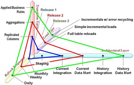
Figure 7.11 Project segmentation lines on a back-end categorized service model.
Embracing rework when it pays
One aspect of the incremental delivery approach that will cause traditional data integration developers to bristle is the notion that a team might deliberately choose to load fact tables when only a few of its dimensions are available. As portrayed in Figure 7.9, the team in our example defined an incremental release that would have only the customer and product dimension ready for use, planning to back fill the revenue fact table later with the keys for the many other dimensions defined for that set of measures. Traditional developers will claim that such an approach only causes unnecessary rework. “It’s just as much effort to link in all the dimensions for a fact table as it is to do one,” they will insist. “So let’s wait until the complete set of dimensions is ready and link them all in at once.”
This might be a compelling argument when true, but it rarely describes the full situation confronting the team. To release fact tables with their full complement of dimensions requires that all the dimensions be developed before fact tables are delivered. Depending on the business circumstance, this can delay the delivery of crucial business insights to the end users for too long a time. It is a return to the big, single delivery paradigm that waterfall methods advocate.
Traditional developers are correct, however. Implementing dimensions incrementally can require significant rework. The degree of rework depends on context. If the new dimensions change the “grain” of the fact table, then the rework can be considerable. The grain of a fact table is the level of atomicity implicit in the table’s data. Measures of sales by sales agent and product are actually aggregates compared to sales by sales agent, product, and customer. If adding new dimensions gives the fact table a deeper grain, then both data transform modules and the end-user dashboards may have to be modified considerably because the new query results will provide a more detailed level of information that the application is already built for.
The amount of rework is also determined by whether the fact tables will be reloaded or have existing data updated in place. The former case is far easier for the team, but if the fact tables contain large data volumes, it can take days to reload them. The alternative is to update already loaded data, but this approach will require the team to program and run data conversion scripts, which takes considerable effort as well.
All the aforementioned considerations support the traditional developer’s view that all the dimensions should be constructed before loading fact tables in order to avoid rework. However, actual conditions can be far less extreme than those considerations suggest. As far as the grain of fact tables is concerned, the additional dimensions often leave the grain of a fact table unaltered. In our example, revenue records are defined by the combination of customer account, billed item, and bill date. Their definition will not change whether or not the billing address is linked to the fact table. Regarding the challenge of already loaded fact table data, projects that are slowly adding source systems, such as occurred in our sample project, start off with small amounts of data, making full reloads less onerous.
In practice, teams will have to provide their product owners with an outline of the cost and benefits of adding dimensions incrementally. The costs are easy to focus upon, but teams must be careful not to overlook the benefits. Data warehouses provide insights into the operational performance of the company. The harm of delaying the availability of a fact table can be that it forces the organization to “fly blind” in the face of such urgent conditions as fast-developing competitive pressures or ruinously large cost overruns. For the telecom company of this chapter’s example, losing 10% of a $15B customer base every quarter represented a revenue fall of over a billion dollars per year. Yes, the rework that adding dimensions incrementally to the revenue fact table may add up to $20,000 or $30,000, but that cost pales in comparison to the opportunity cost of not understanding the forces driving customers away.
Compelling business situations usually lead agile data warehousing teams into project segmentation plans that involve an appreciable amount of deliberate rework. The true objective of the agile team should be not to eliminate rework, but to avoid design churn, which can be defined as needless modification in construction plans due to mistakes in requirements and analysis. In the approach outlined in the past few chapters, the agile team has followed disciplined enterprise architectural planning guidelines by pursuing business modeling before logical modeling, and logical modeling before physical design. The recommended decomposition of the agile epics and themes established user stories before developer stories, which aligns with business modeling before logical design. As long as agile teams persist in this ordering of their analysis, they will reduce project rework to its practical minimum. The rework that remains will make business sense, as long as the opportunity gained by an early release outweighs the extra cost of delivering the solution in increments. By planning on incremental deliveries and the rework it entails, the data warehousing team will be able to meet one of the primary goals of agile methods: a delivery process through which the business stakeholders constantly receive new value from the development team.
Summary
The infrequent attention that waterfall methods pay to estimating project labor leads regularly to grossly inaccurate project estimates that hurt both developers and stakeholders alike. In contrast, because agile methods build estimating into the fabric of every development iteration, it quickly makes developers capable of estimating accurately and maintains their skills. To bolster the accuracy of their predictions, an agile team estimates using two units of measures—story points and labor hours, cross-checking and revising both viewpoints until their predictions agree.
Agile also provides the notion of sized-base estimation using a technique called estimating poker that allows teams to assign story points to backlog stories quickly. Being fast and accurate, this forecasting technique enables a team to estimate the stories of both an iteration and an entire project, allowing agile teams to predict how many iterations a project will require. Because all aspects of the developer’s collaboration must go right for teams to regularly deliver upon all that they estimate they can build each iteration, tracking the accuracy of a team’s estimates can quickly reveal adverse changes in the collaboration patterns within a project room.
The ability to estimate a full project accurately enables agile teams to group the stories on a backlog into a series of intermediate releases. There are three techniques for planning this project segmentation: divisions drawn upon the application’s star schema, its tiered integration data model, and its categorized service model. Proper project segmentation may well include some deliberate rework, which—far from being the anathema that traditional software engineers may regard it—makes perfect business sense when it allows teams to deliver crucial analytical capabilities to end users early and often.