Reinforcement learning is an area of machine learning that searches for the behavior of an agent when performing actions in a particular environment. The objective of the behavior is to maximize the notion of cumulative reward by identifying the best action to take for a given environment.
Machine learning is an application of artificial intelligence that provides a system the ability to automatically learn and improve from experience without being explicitly programmed. Reinforcement learning (RL) is an area of machine learning that has made significant contributions in various areas, including robotics and video games. RL is about taking a suitable action to maximize reward in a particular situation.
This chapter illustrates the use of visualization to highlight how reinforcement learning operates on a simple example. This chapter provides a generic implementation of reinforcement learning, called Q-Learning, and proposes some visualizations to help illustrate the execution of the algorithm. The chapter is self-contained by providing the complete implementation of Q-Learning and a small game as an illustration.
This chapter is relatively long and illustrates the use of a number of Roassal components:
Mondrian is a high-level API to build visual graphs. The Roassal3-Mondrian package contains the whole implementation of Mondrian and numerous examples.
Chart is a high-level API to build charts. The Roassal3-Chart package contains all the basic infrastructure to build charts.
Integration in the Inspector to have multiple visualizations of the same object. All the examples in this chapter are meant to be executed in the Playground, using Cmd+G or Alt+G, which opens an Inspector pane. I recommend you read Chapter 13 before reading this chapter.
This chapter uses reinforcement learning on a simple and intuitive example, which is a small knight trying to find the exit without encountering monsters. The game is very simple, but it illustrates the need for some visualizations to better understand how Q-Learning, the algorithm used in this implementation, operates.
Reinforcement learning computes the cumulative rewards over a sequence of actions. An exploration step is called an episode. Q-Learning and the game implementation span over three classes:
RLGrid defines a grid, which is a simple square area that contains the exit and some monsters.
RLState defines a state, consisting of a grid and the position of the knight.
RL implements Q-Learning, the reinforcement learning algorithm.
Defining the Map
The RLGrid class represents the map in which the knight can move around. The grid is a simple matrix containing characters. To encode the content of the map, use the following conventions:
$e represents the exit. The knight is looking for the exit to finish the game.
$m represents a monster. The knight has to learn to avoid monsters.
$. represents an empty cell. The knight can freely move on an empty cells.
RLGrid is defined as follows:
Object subclass: #RLGrid
instanceVariableNames: 'content'
classVariableNames: ''
package: 'ReinforcementLearning'
The class defines a variable called content, which is a two-dimensional array of characters. A grid is initialized using the following:
RLGrid>>initialize
super initialize.
self setSize: 2
By default, a grid is a square of two cells per side. The setSize: method creates the following map:
RLGrid>>setSize: anInteger
"Set the grid as a square of size anInteger, containing the character $."
To keep this code relatively short to fit in a chapter, it uses a number of conventions. The character $. represents a space in which the knight can move around freely. The content of the map may be modified using a number of utility methods. The atPosition: method returns a character contained at a particular position:
RLGrid>>atPosition: aPoint
"Return the character located at a given position"
^ (content at: aPoint y) at: aPoint x
The map can be modified using the atPosition:put: method, defined as follows:
RLGrid>>atPosition: aPoint put: aCharacter
"Set the aCharacter (value of a cell map) at a given position"
^ (content at: aPoint y) at: aPoint x put: aCharacter
The exit of the map is set using a dedicated method, invoked by initialize:
RLGrid>>setExitBottomRight
"Set the exit position at the bottom right of the grid"
self atPosition: self extent put: $e
The extent of the grid is obtained using:
RLGrid>>extent
"Return a point that represents the extent of the grid"
^ content first size @ content size
Monsters are defined in a map using the setMonsters: method. This method takes as an argument the number of monsters to add, and it is defined as follows:
RLGrid>>setMonsters: numberOfMonstersToAdd
| random leftMonsters s pos nbTries |
random := Random seed: 42.
leftMonsters := numberOfMonstersToAdd.
nbTries := 0.
s := self extent.
[ leftMonsters > 0 ] whileTrue: [
pos := (random nextInteger: s x ) @ (random nextInteger: s y).
(self atPosition: pos) = $.
ifTrue: [
nbTries := 0.
self atPosition: pos put: $m.
leftMonsters := leftMonsters - 1 ]
ifFalse: [
nbTries := nbTries + 1.
nbTries > 5 ifTrue: [ ^ self ] ]
]
The method locates a number of monsters on the map. The method uses a number generator with a seed to deterministically generate a map. The method tries to locate monsters at random positions. If there are too many monsters, the method exits after a number of tries.
You now have to consider a technical aspect of the way Q-Learning is implemented. Grid objects need to be structurally compared to determine whether a particular state was already discovered. Consider this expression:
(RLGrid new setSize: 2; setMonsters: 3) = (RLGrid new setSize: 2; setMonsters: 3)
At that stage of the implementation, this expression returns false, even if the structures of the two grids are identical:
The two grids have the same size
The two grids have the same number of monsters
Those monsters are located at exactly the same locations, thanks to the seed number defined in the setMonsters: method you saw earlier
This expression returns false as it’s the result of comparing the object identity (i.e., the address in memory of the object). Since evaluating (RLGrid new setSize: 2; setMonsters: 3) returns a new object, performing the = operation between two different objects will return false. However, in this situation, you want the comparison to return true since you are comparing two instances of the identical map. As such, the = needs to operate on the structure of the objects, and not on the object identity, as it does by default. You therefore have to redefine the = and hash methods (these two methods are highly intertwined).
The equality can be redefined as follows:
RLGrid>>= anotherObject
"Return true if anotherObject is the same map than myself"
anotherObject class == self class ifFalse: [ ^ false ].
^ content = anotherObject content
Two objects are equal if their class and contents are the same. The contents of a grid are obtained with this method:
RLGrid>>content
"Return the grid content, as an array of array of characters"
^ content
Objects can also be compared through their hash values: two objects that are considered equal (i.e., comparing them with = returns true) must have the same hash value. Hash values are intensively used in dictionaries. The QTable is an essential component of the Q-Learning algorithm that maps states and actions to a reward. It is useful to store what the algorithm is learning. In this example, you will model the QTable as a dictionary, and as such, a grid needs to have a proper hash function. Luckily, defining such a hash function is simple in this case:
RLGrid>>hash
"The hash of a grid is the hash of its content"
^ content hash
After having implemented this method, the following expression evaluates to true:
(RLGrid new setSize: 2; setMonsters: 3) = (RLGrid new setSize: 2; setMonsters: 3)
New states are created during the exploration of the grid. A copy of the grid is associated with each new state, and you need a way to copy a grid. Pharo provides an easy way to copy any object, by simply defining the postCopy method:
RLGrid>>postCopy
"A grid must be properly copied"
super postCopy.
content := content copy
You can visualize a grid to see the result of the reinforcement learning algorithm. Define a simple method that defines a grid of boxes:
o = $. ifTrue: [ s color: Color veryVeryLightGray ].
o = $m ifTrue: [ s color: Color lightRed ].
o = $e ifTrue: [ s color: Color lightYellow ].
].
canvas addAll: shapes.
RSGridLayout new gapSize: 0; lineItemsCount: (self extent x); on: shapes.
shapes translateTopLeftTo: 0 @ 0.
^ canvas
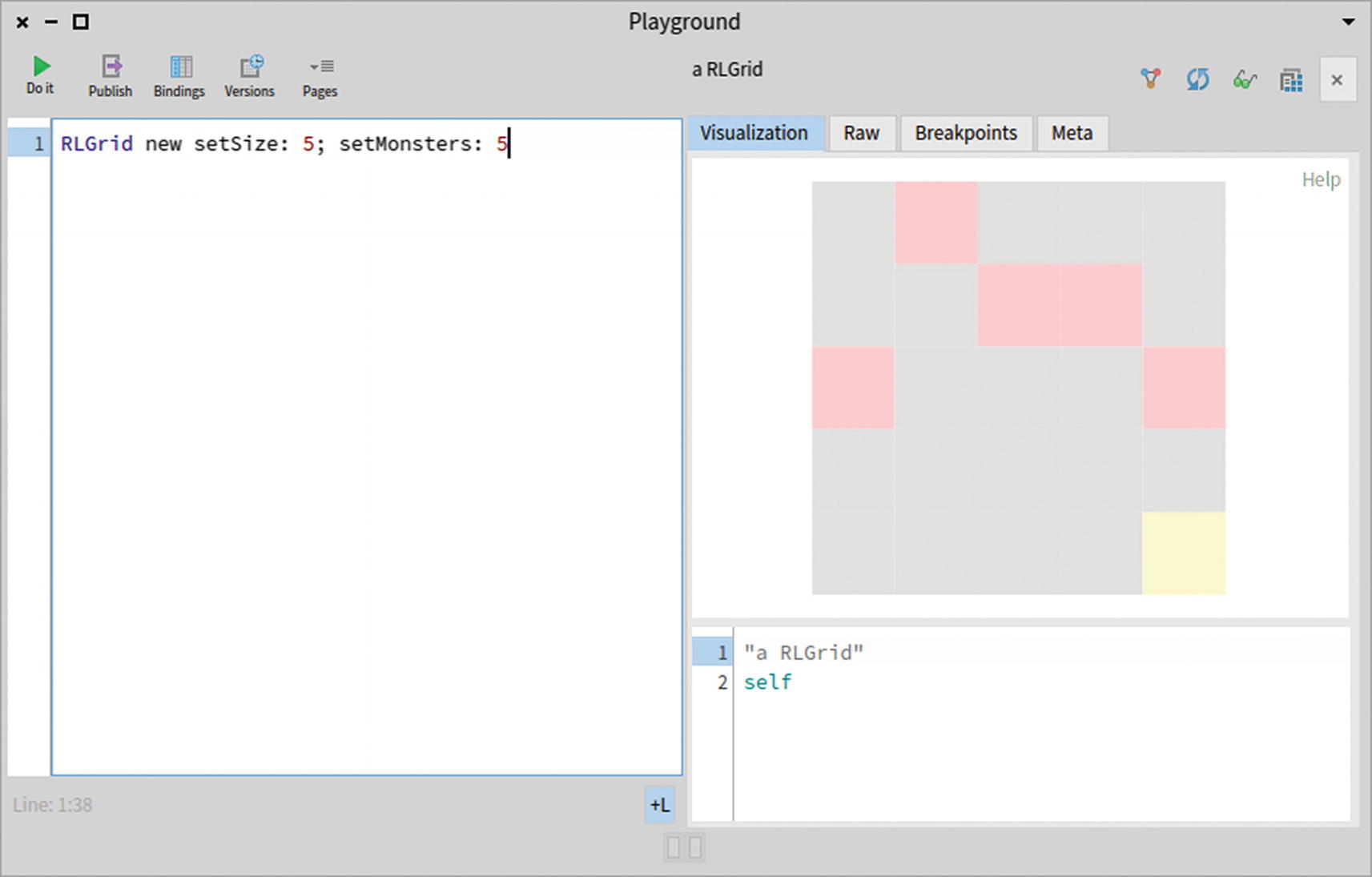
Each cell of the map is represented as a small, squared box. The color of each box indicates what the cell actually represents. A space is represented as a gray box, a monster is a red box, and the exit is a yellow box. You can make the Inspector show the visualization defined on a grid by simply defining the following:
You can now inspect the following expression by pressing Cmd+G or Alt+G in the Playground (see Figure 14-1):
RLGrid new setSize: 5; setMonsters: 5
Figure 14-1
Inspecting a grid
Modeling State
Modeling the state is the second main component of this chapter. A state is a combination of a grid with a position of the knight. The reinforcement learning algorithm operates by discovering states; the actions taken by the knight are expressed using state transitions. The RLState class is defined as follows:
Object subclass: #RLState
instanceVariableNames: 'grid position'
classVariableNames: ''
package: 'ReinforcementLearning'
The default position of the knight is set in the initialize method:
RLState>>initialize
super initialize.
position := 1 @ 1
A grid can be set to a state using the following:
RLState>>grid: aGrid
"Set the grid associated to the state"
grid := aGrid
A grid can be obtained from a state using the following:
RLState>>grid
"Return the grid associated to the state"
^ grid
The position of the knight can be set using the following:
RLState>>position: aPoint
"Set the knight position"
position := aPoint
The knight’s position is fetched using the following:
RLState>>position
"Return the knight position"
^ position
Similar to RLGrid, a state needs to be compared with other states. Define the following method:
RLState>>= anotherState
"Two states are identical if (i) they have the same class, (ii) the same grid, and (iii) the same position of the knight"
anotherState class == self class ifFalse: [ ^ false ].
^ grid = anotherState grid and: [ position = anotherState position ]
The hash value of a state can be obtained using the following:
RLState>>hash
"The hash of a state is a combination of the hash of the grid with the hash of the position"
^ grid hash bitXor: position hash
Obtaining a string representation of a state is handy, especially to represent the QTable:
RLState>>printOn: str
"Give a string representation of a state"
str nextPutAll: 'S<'.
str nextPutAll: self hash asString.
str nextPutAll: '>'.
The printOn: method produces a string that can be used as a textual label for the state. For example, the RLState new printString expression returns a string called 'S<376548926>'. The numerical value depends on the internal state of the Pharo virtual machine, so you will likely have a different value.
You can now focus on the visualization of the state. The visualize method simply renders the grid and the position of the knight, and it is defined as follows:
RLState>>visualize
"Visualize the grid and the knight position"
| c knightShape |
c := grid visualize.
knightShape := RSCircle new size: 15; color: Color blue lighter lighter.
c add: knightShape.
knightShape translateTo: self position - (0.5 @ 0.5) * 20.
^ c
The visualization can now be hooked into the Inspector’s framework:
You can now try the visualization by using Cmd+G/Alt+G on the following script (see Figure 14-2):
RLState new
grid: (RLGrid new setSize: 5; setMonsters: 5)
Figure 14-2
Visualizing a state
The squared map is five cells wide, the monsters are in light red, and the exit is in yellow.
The Reinforcement Learning Algorithm
The third component of this chapter is the reinforcement algorithm engine itself. The RL class is large and contains many algorithmic parts for which the chapter provides the code without expanding on its rationale. The goal of this chapter is to illustrate how visualizations are beneficial when using reinforcement learning. As such, this chapter is not a tutorial about reinforcement learning. The good news is that there are not many technical parts. First define the RLclass as follows:
startState defines the starting state of the algorithm. Each episode (unit of exploration in RL) starts from this state.
r is a random number generator, initialized with a fixed seed to enable determinism and reproducibility.
numberOfEpisodes indicates the number of episodes the algorithm has to run for. This value can be considered the amount of exploration the algorithm needs to conduct.
maxEpisodeSteps indicates the number of steps the knight needs to make during each episode. You need to make sure that this number is large enough to allow the knight to find the exit.
minAlpha indicates the minimum value of the decreasing learning ramp.
gamma represents the discount of the reward.
epsilon represents the probability of choosing a random action when acting.
qTable is a dictionary that models the QTable and contains states as keys and rewards as values (each actions is associated with a reward).
rewards lists the accumulated rewards obtained along the episodes. This list indicates how “well” the algorithm is learning.
path represents the path of the knight to exit the grid.
stateConnections describes all the transitions between the states.
As mentioned, this class has a mathematical complexity that is not included here. Only a brief description is provided, leaving the job of detailing how Q-Learning operates for another book. The initialization of an RL object is performed using the following:
RL>>initialize
super initialize.
r := Random seed: 42.
numberOfEpisodes := 20.
maxEpisodeSteps := 100.
minAlpha := 0.02.
gamma := 1.0.
epsilon := 0.2.
qTable := Dictionary new.
rewards := OrderedCollection new.
path := OrderedCollection new.
stateConnections := OrderedCollection new.
The number of episodes can be set using the following:
RL>>numberOfEpisodes: aNumber
"Set the number of exploration we need to perform"
numberOfEpisodes := aNumber
The propensity for exploring the world versus taking the best action is set by the epsilon value:
RL>>epsilon: aFloat
"Set the probability to explore the world. The argument is between 0.0 and 1.0. A value close to 0.0 favors choosing an action that we know is a good one (thus reducing the exploration of the grid). A value close to 1.0 favors the world exploration instead."
epsilon := aFloat
Set the maximum number of steps for each episode as follows:
RL>>maxEpisodeSteps: anInteger
"Indicate how long an exploration can be"
maxEpisodeSteps := anInteger
The value of maxEpisodeSteps has a default value of 100, as mentioned in initialize. This value is high enough for maps having fewer than 100 cells (i.e., a grid smaller than 10 x 10).
For a given state and action, you must determine the behavior of the knight, compute the reward gained by performing the action, and indicate whether the game is over. Define the act:action: method for that purpose:
newState := RLState new grid: newGrid; position: p.
stateConnections add: aState -> newState.
^ { newState . reward . isDone }
The knight can move by one cell in any of the four directions. A move is represented as an action, itself described as a numerical value ranging from 1 to 4. Define the actions method, which simply returns the list of the actions:
RL>>actions
"Return the considered actions"
^ #(1 2 3 4)
You represent an action as a number since it is convenient to access the Q values from the QTable. For a given state, the knight needs to take an action. Either this action is random or it is based on the exploration made by the knight. The chooseAction: method is designed for that purpose:
RL>>chooseAction: state
"Choose an action for a given state"
^ r next < epsilon
ifTrue: [ self actions atRandom: r ]
ifFalse: [
"Return the best action"
(self qState: state) argmax ]
Once an action has been determined, the knight needs to move accordingly. It is important for the knight to not exit the grid:
RL>>moveKnight: state action: action
"Return the new position of a car, as a point. The action is a number from 1 to 4.
^ ((state position + delta) min: state grid extent) max: 1 @ 1
Once the knight has explored enough, you can use what it has learned to find the exit. The play method determines a list of actions to be taken to reach the exit:
This method implements the Bellman equation, which is the core of the algorithm. The algorithm decays the learning rate alpha at every episode. As the knight explores more of the environment, it will believe that there is not much to learn.
To simplify the examples you will see shortly, you can define the setInitialGrid: method to set the grid in the starting state:
RL>>setInitialGrid: aGrid
"Set the grid used in the initial state"
startState := RLState new grid: aGrid
The core of reinforcement learning algorithm is now implemented. You just need to define methods to visualize some aspects of the algorithm’s executions. First the QTable is an important aspect of the algorithm to visualize. Define the visualizeQTable method for that purpose:
RL>>visualizeQTable
| c state values allBoxes sortedAssociations |
c := RSCanvas new.
c add: (RSLabel text: 'State').
c add: (RSLabel text: '^').
c add: (RSLabel text: 'V').
c add: (RSLabel text: '<').
c add: (RSLabel text: '>').
sortedAssociations := qTable associations reverseSortedAs: [ :assoc | assoc value average ].
sortedAssociations do: [ :assoc |
state := RSLabel model: assoc key.
values := RSBox
models: (assoc value collect: [ :v | v round: 2 ])
forEach: [ :s :m | s extent: 40 @ 20 ].
c add: state.
c addAll: values.
].
RSCellLayout new lineItemsCount: 5; gapSize: 1; on: c shapes.
allBoxes := c shapes select: [ :s | s class == RSBox ].
RSNormalizer color
shapes: allBoxes;
from: Color red darker darker; to: Color green darker darker;
normalize.
allBoxes @ RSLabeled middle.
^ c @ RSCanvasController
The method represents the QTable as a table in which columns are the rewards per actions, and each row is a state. You use a cell layout to locate all the values in the grid. The cell layout arranges all the shapes to be lined up, both vertically and horizontally. This visualization is hooked into the Inspector using the following:
RL>>inspectorQTable
<inspectorPresentationOrder: 90 title: 'QTable'>
^ SpRoassal3InspectorPresenter new
canvas: self visualizeQTable;
yourself
The evaluation panel is not relevant in this case and can be removed using the following:
RL>>inspectorQTableContext: aContext
aContext withoutEvaluator
The evolution of the rewards along the episodes can be represented using a chart. The visualizeReward method uses the Chart component of Roassal:
RL>>visualizeReward
| c plot |
c := RSChart new.
plot := RSLinePlot new.
plot y: rewards.
c addPlot: plot.
c addDecoration: (RSChartTitleDecoration new title: 'Reward evolution'; fontSize: 20).
c xlabel: 'Episode' offset: 0 @ 10.
c ylabel: 'Reward' offset: -20 @ 0.
c addDecoration: (RSHorizontalTick new).
c addDecoration: (RSVerticalTick new).
c build.
^ c canvas
The chart to visualize the reward is composed of a line plot. You plot all the values contained in the rewards variable. A number of decorations are added to improve the appearance of the chart. The two axes have a label and some ticks. The reward visualization is integrated in the Inspector with the following:
RL>>inspectorReward
<inspectorPresentationOrder: 90 title: 'Reward'>
^ SpRoassal3InspectorPresenter new
canvas: self visualizeReward;
yourself
Since there is no need for an evaluation pane, you can disable it:
RL>>inspectorRewardContext: aContext
aContext withoutEvaluator
The path of the knight can be visualized using the following method:
RL>>visualizeResult
"Assume that the method play was previously invoked"
| c s |
self play.
c := startState visualize.
path do: [ :p |
s := RSCircle new size: 5; color: Color blue lighter lighter.
c add: s.
s translateTo: p - (0.5 @ 0.5) * 20.
].
^ c @ RSCanvasController
The integration in the Inspector is done using the following:
RL>>inspectorResult
<inspectorPresentationOrder: 90 title: 'Result'>
^ SpRoassal3InspectorPresenter new
canvas: self visualizeResult;
yourself
Since there is no need to have an evaluation pane when looking at the result, you can disable it using the following:
RL>>inspectorResultContext: aContext
aContext withoutEvaluator
Generally speaking, a graph is a set of nodes connected by edges. In this context, the reinforcement learning algorithm builds a graph made of states and actions connecting those states. Exploring the map is expressed by adding new states to the graph, and identifying an ideal path through the map is the result of determining adequate rewards for each action and each state. Visualizing the graph built by the algorithm is relevant to understanding how the exploration went during the learning phase. You therefore need to build the visualizeGraph method:
RL>>visualizeGraph
| s allStates d m |
s := stateConnections asSet asArray.
d := Dictionary new.
s do: [ :assoc |
(d at: assoc key ifAbsentPut: [ OrderedCollection new ]) add: assoc value ].
allStates := qTable keys.
m := RSMondrian new.
m shape circle.
m nodes: allStates.
m line connectToAll: [ :aState | d at: aState ifAbsent: [ #() ] ].
m layout force.
m build.
^ m canvas.
The visualizeGraph method uses the RSMondrian class, which is a very useful class offered by Roassal to build graphs. A circle shape is selected using m shape circle. During the learning phase, the stateConnections variable is filled with all the associations between states and the qTable variable is filled with the rewards associated with each action. The qTable key expression returns all the states that were created during the learning phase. For a given state aState, the expression d at: aState ifAbsent: [ #()] returns the list of connected states (i.e., a directed going from aState to the connected states).
The graph can be accessible from the Inspector using the following method:
Since an evaluator context does not make much sense to have for visualizeGraph, you can remove it using the method:
RL>>inspectorGraphContext: aContext
aContext withoutEvaluator
You can define a complementary visualization to associate some metrics with each state. Consider the following script:
RL>>visualizeWeightedGraph
| s allStates d m |
s := stateConnections asSet asArray.
d := Dictionary new.
s do: [ :assoc |
(d at: assoc key ifAbsentPut: [ OrderedCollection new ]) add: assoc value ].
allStates := qTable keys.
m := RSMondrian new.
m shape circle.
m nodes: allStates.
m line connectToAll: [ :aState | d at: aState ifAbsent: [ #() ] ].
m normalizeSize: [ :aState | (qTable at: aState) average ] from: 5 to: 30.
m normalizeColor: [ :aState | (qTable at: aState) max ] from: Color gray to: Color green.
m layout force.
m build.
^ m canvas.
The visualization defined in visualizeWeightedGraph is very similar to the one in visualizeGraph. The only difference is that it has some metrics associated with the size and color of each state. The size of a state indicates the average reward on the four actions: the higher the average is, the larger the state. As such, a large state contributes to reaching the exit.
The color of a state indicates the maximum reward among the four actions: if an action with a high reward (e.g., if the knight is next to the exit) can be performed on a state, this state will be colored in green. The weighted graph visualization is hooked into the Inspector using the following:
RL>>inspectorWeightedGraph
<inspectorPresentationOrder: 90 title: 'Weighted state graph'>
^ SpRoassal3InspectorPresenter new
canvas: self visualizeWeightedGraph;
yourself
Since there is no need to have the evaluation pane, you can disable it:
RL>>inspectorWeightedGraphContext: aContext
aContext withoutEvaluator
You have now implemented the whole reinforcement learning algorithm and four visualizations:
Result visualization shows the path taken by the knight to escape the grid.
QTable renders the Q table, in which each cell of the matrix contains the reward of an action in a given state.
State graph renders the graph explored by the algorithm (states are nodes and actions are edges).
Weighted state graph highlights the importance of the state to contribute to exiting the grid.
The visualization is accessible when inspecting an instance of the RL class.
Running the Algorithm
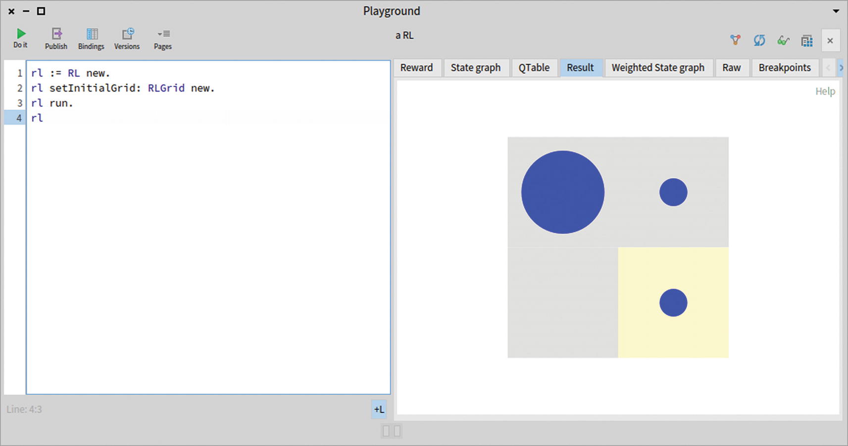
Now that you have implemented the reinforcement learning algorithm and have added the necessary script to have the knight exit the grid, it is time to try it out! Evaluate the following code snippet in the Playground by pressing Cmd+G/Alt+G (see Figure 14-3):
rl := RL new.
rl setInitialGrid: RLGrid new.
rl run.
rl
Figure 14-3
Reaching the exit in the simplest possible grid
Evaluating the script split the Playground in two. The right side of the Playground inspects the result of executing the script, an RL object in this case. The grid used in the example has a side of two cells, and no monster inhabits the map. The large blue dot indicates the initial position of the knight and the smaller dots indicate the path. In Figure 14-2, you can see that the knight needs to move two cells to reach the yellow cell, which represents the exit.
The example seems trivial, but actually, it is not. If you closely look at the program, you never “told” the knight that it has to exit the map! The knight discovered that exiting the map is the best way to maximize the cumulative reward. By randomly choosing some actions, it discovered the map. Note that the only cell the knight can see is the one that it’s standing on.
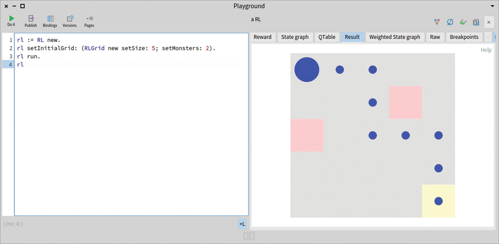
Now try running the reinforcement learning algorithm on a larger example. Consider the following code snippet (see Figure 14-4):
rl := RL new.
rl setInitialGrid: (RLGrid new setSize: 5; setMonsters: 2).
rl run.
rl
Figure 14-4
Exiting the grid while avoiding monsters
Figure 14-4 shows the path taken by the knight to exit the map while avoiding the two monsters. Selecting the Reward tab shows the evolution of the reward along the episodes (see Figure 14-5).
Figure 14-5
The reward evolution indicates that the algorithm is learning
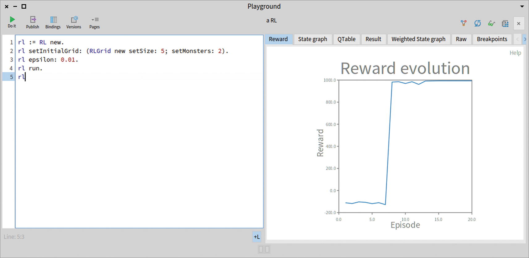
The reinforcement learning algorithm balances the exploration of the map versus taking good actions that were previously learned. Figure 14-5 shows sudden drops in the reward evolution. This indicates an accumulation of explorations that lead the knight to bump into monsters, the result of some random explorations. The epsilon value indicates the likelihood to explore the map: a low value (i.e., positive float number close to 0) indicates little exploration, favoring recalling what it has learned. Having a high epsilon (i.e., a float value slightly below 1.0) favors random exploration. You can verify the effect of epsilon using the following script (see Figure 14-6):
rl := RL new.
rl setInitialGrid: (RLGrid new setSize: 5; setMonsters: 2).
rl epsilon: 0.01.
rl run.
rl
Figure 14-6
Reducing the epsilon value prevents sudden drops in the reward evolution
The default value of epsilon is 0.2, as defined in the initialize method. Setting a significantly smaller value, such as 0.01 in the script, reduces the discovery of new path in favor of reusing what the knight has learned. As such, there is no sudden drop in the reward evolution chart. Having the reward at a high level indicates that the Q-Learning has actually learned the best action to take in the relevant states.
The State Graph tab in the Playground represents the graph composed of the explored states (see Figure 14-7).
Figure 14-7
Graph illustrating the connections between the states discovered by the reinforcement learning algorithm
A state is a combination of a grid and a position. The graph shown in Figure 14-7 has the shape of a square. This indicates that the knight has visited every position of the map, even the one containing the monsters. If you reduce the amount of iterations used when running the algorithm, fewer states will be discovered. You can verify this using the new script (see Figure 14-8):
rl := RL new.
rl setInitialGrid: (RLGrid new setSize: 5; setMonsters: 2).
rl epsilon: 0.01.
rl numberOfEpisodes: 7.
rl run.
rl
Figure 14-8
Reducing the exploration is translated into discovering fewer states
The number of episodes set by default is 20, as indicated in the initialize method. Reducing this value to 7 implies fewer iterations when running the algorithms, and as such, fewer states are discovered. Figure 14-8 indicates this situation by having fewer nodes and fewer edges. Note that the knight cannot find the exit of the map.
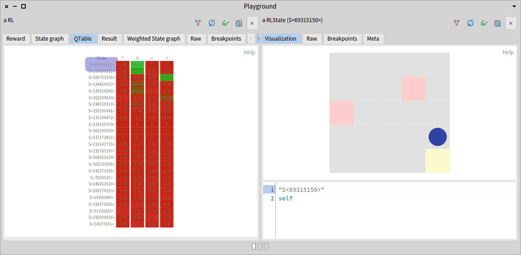
The QTable tab shows the matrix of the reward values for a state and an action (see Figure 14-9).
Figure 14-9
The QTable matrix
The red indicates the actions that are not beneficial. A state can be inspected by clicking it. The first state has a green instance action, representing the action to go down. Clicking it reveals that the state corresponds to when the knight is just above the exit. Going down one cell in that case leads to a very high reward (see Figure 14-10).
Figure 14-10
States in the QTable can be inspected by clicking them
The weighted state graph illustrates the relevance of a state to contribute to reaching the exit. Consider the script given previously (see Figure 14-11):
rl := RL new.
rl setInitialGrid: (RLGrid new setSize: 5; setMonsters: 2).
rl run.
rl
Figure 14-11
Normalized metrics applied to the graph of states
Large green circles represent states that contribute to maximizing the cumulative reward and therefore reaching the exit.
What Have You Learned in This Chapter?
This chapter detailed a compelling case study for using visualizations. Q-Learning is a very popular algorithm that belongs to the family of reinforcement learning. Q-Learning, as with most machine learning algorithms, is best understood with visual representations. The visualizations were realized using dedicated and expressive components. This chapter included:
An illustration of using Mondrian to build and render graphs.
Shapes in the Mondrian graph normalized using some metrics.
Chart built using the API provided by Roassal.
A complete implementation of the Q-Learning algorithm with a classic scenario.