This chapter provides an overview of Roassal, as well as a few examples. The chapter does not go into detail since that is something that will occur in forthcoming chapters. Many short code snippets are provided and briefly described. You can copy and paste these snippets directly into Pharo and each one illustrates a particular aspect of the Roassal platform.
It is important to keep in mind that this chapter is just a tour of Roassal and Pharo. If you are not familiar with Pharo, you might find the amount of code given here a bit confusing. The next chapter serves as an introduction of the Pharo language and explains many aspects of the language syntax.
Roassal is the framework for the Pharo programming language. As such, the first step to try the examples given in this chapter is to install Pharo. The Pharo website provides all the necessary instructions to do so (https://pharo.org/download). Pharo can be installed directly via the command line or using the Pharo launcher. Both ways are equivalent and you may prefer one over the other based on your personal workflow.
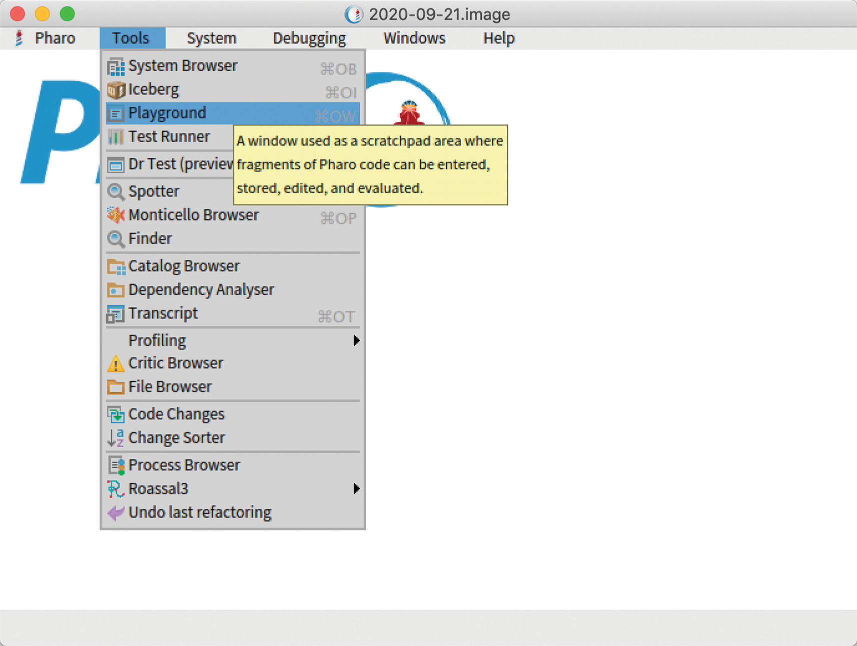
Once you have installed Pharo, you need to open the Playground, which is a tool offered by Pharo to execute code. You can think of the Playground as a UNIX terminal. The Playground is opened from the top toolbar, as shown in Figure 2-1.
Figure 2-1
Opening the Playground from the World menu
After selecting Playground from the menu, you’ll see a window in which you can type any Pharo instructions. Just type the following instructions (or copy and paste them if you are reading an electronic version of this book):
You can execute the code by pressing Cmd+D (if you are a macOS user) or Ctlr+D (for Windows and UNIX users), or by pressing the green Do It button.
Loading Roassal should take a few seconds, depending on your Internet connection. Once it’s loaded, you may want to save your Pharo environment (a.k.a, the image in the Pharo jargon) by choosing Pharo➤Save from the toolbar menu. You are now ready to try your first visualization.
First Visualization
Most of the visualizations in this book are written as short scripts, directly executable in the Playground. You can open a new Playground or simply reuse an already open Playground (e.g., the one you used to load Roassal). In that case, you should erase the contents of the Playground and paste in the new script.
Evaluate the following example in the Playground (see Figure 2-2).
c := RSCanvas new.
1 to: 100 do: [ :i |
c add: (RSLabel new model: i) ].
RSLineBuilder line
shapes: c nodes;
connectFrom: [ :i | i // 2 ].
RSClusterLayout on: c nodes.
c @ RSCanvasController.
c open
Figure 2-2
Connecting numbers
The script begins by creating a canvas using the RSCanvas class. The script adds 100 labels to the canvas, each representing a number between 1 and 100. Lines are built as follows: for each number i between 1 and 100, a line is created from the element representing i //2 and i. The expression a //b returns the quotient between a and b, e.g., 9 //4 = 2 and 3 //2 = 1. Nodes are then ordered using a cluster layout.
As a short exercise, you can replace 100 with any other value. You can also replace the RSClusterLayout class with RSRadialTreeLayout, RSTreeLayout, or RSForceBasedLayout.
Visualizing the Filesystem
You will reuse the previous visualization to visualize a filesystem instead of arbitrary numbers. Pharo offers a complete library to manipulate files and folders. Integrating files into a Roassal visualization is easy. Consider the following script:
path := '/Users/alexandrebergel/Desktop'.
extensions :=
{ 'pdf' -> Color red . 'mov' -> Color blue } asDictionary.
Figure 2-3 shows the contents of the path /Users/alexandrebergel/Desktop, which correspond to the contents of the desktop on macOS. The path variable contains a location on your filesystem. Obviously, you need to change the path to execute the script. Note that indicating a large portion of the filesystem may significantly increase the computation time since recursively fetching file information is time-consuming. The path asFileReference expression converts a string indicating a path as a file reference. FileReference is a Pharo class that represents a file reference, typically locally stored on hard disk. The allChildren message gets all the files recursively contained in the path. The visualization paints files whose names end with .pdf in red and paints all videos files ending with .mov in blue.
Figure 2-3
Visualizing the filesystem
Compared to the previous example, this visualization uses a normalizer to give each circle a size according to the file size. The size varies from 10 to 30 pixels, and it uses a square root (sqrt) transformation to cope with disparate sizes.
As an exercise, you can extend the color schema for specific files located on your filesystem. Color rules must follow the pattern 'pdf'-> Color red and must be separated by a period character.
Charting Data
Roassal offers a sophisticated library to build charts. Consider the following example, showing the high of the COVID-19 pandemic during its first 250 days (see Figure 2-4).
chart addDecoration: (RSHorizontalTick new fontSize: 10).
chart addDecoration: (RSVerticalTick new integerWithCommas; fontSize: 10).
chart ySqrt.
chart build.
b := RSLegend new.
b container: chart canvas.
countries with: chart plots do: [ :c : p |
b text: c withBoxColor: (chart colorFor: p) ].
b layout horizontal gapSize: 30.
b build.
b canvas open
Figure 2-4
The first 250 days of the pandemic in 2020
The url variable points to a dataset that contains the first 250 days of the COVID-19 pandemic in 2020 caused by the SARS-CoV-2. Note that we split the URL to accommodate the book formatting. The data stored in the covidDataUntil23-September-2020.txt file is a simple serialization of the data to be rendered by the charter. The RSChart class is the entry point of the charting library. Plots are added to a chart and a few decorations are added. A legend is located below to associate curves with countries.
Sunburst
A sunburst is a visualization designed to represent hierarchical data structure. Consider the following example (Figure 2-5).
sb := RSSunburstBuilder new.
sb sliceShape withBorder.
sb sliceColor: [ :shape | shape model subclasses isEmpty
ifTrue: [ Color purple ]
ifFalse: [ Color lightGray ] ].
sb explore: Collection using: #subclasses.
sb build.
sb canvas @ RSCanvasController.
RSLineBuilder sunburstBezier
width: 2;
color: Color black;
markerEnd: (RSEllipse new
size: 10;
color: Color white;
withBorder;
yourself);
canvas: sb canvas;
connectFrom: #superclass.
sb canvas open
Figure 2-5
Visualizing the collection class hierarchy using a sunburst
This sunburst is a software visualization. Each arc represents a class, and the nesting indicates class inheritance, which is highlighted with Bezier lines.
Graph Rendering
Roassal offers a wide range of tools to manipulate and render graphs. Consider the following script (see Figure 2-6).
line markerEnd: (RSShapeFactory arrow size: length * 2).
line markerEnd offset: length / -5.
].
(canvas nodes, canvas lines) @ (RSLabeled new
in: [ :lbl |
lbl location middle.
lbl shapeBuilder labelShape color: Color black ];
yourself).
RSForceBasedLayout new charge: -500; doNotUseProgressBar; on: nodes.
canvas @ RSCanvasController.
canvas open
Figure 2-6
Visualizing a graph
Nodes considered in the graph represent characters ranging from $a to $s. The edges variable defines the weighted connections between nodes. The script renders the graph using labeled arrow lines and uses a force-based layout. Furthermore, moving the mouse above a node highlights lines connected to it.
What Have You Learned in This Chapter?
Many examples are available in the Roassal distribution, in the Roassal3-Examples package. Hundreds of examples cover many different parts of Roassal. Many relevant topics in Roassal are illustrated by more than one example to illustrate its flexibility and the capability to configure.
Some of the examples in this chapter are covered in-depth in coming chapters. I recommend you experiment by adapting and tweaking these examples.