Chapter Five. Recursion and Trees
The concept of recursion is fundamental in mathematics and computer science. The simple definition is that a recursive program in a programming language is one that calls itself (just as a recursive function in mathematics is one that is defined in terms of itself). A recursive program cannot call itself always, or it would never stop (just as a recursive function cannot be defined in terms of itself always, or the definition would be circular); so a second essential ingredient is that there must be a termination condition when the program can cease to call itself (and when the mathematical function is not defined in terms of itself). All practical computations can be couched in a recursive framework.
The study of recursion is intertwined with the study of recursively defined structures known as trees. We use trees both to help us understand and analyze recursive programs and as explicit data structures. We have already encountered an application of trees (although not a recursive one), in Chapter 1. The connection between recursive programs and trees underlies a great deal of the material in this book. We use trees to understand recursive programs; we use recursive programs to build trees; and we draw on the fundamental relationship between both (and recurrence relations) to analyze algorithms. Recursion helps us to develop elegant and efficient data structures and algorithms for all manner of applications.
Our primary purpose in this chapter is to examine recursive programs and data structures as practical tools. First, we discuss the relationship between mathematical recurrences and simple recursive programs, and we consider a number of examples of practical recursive programs. Next, we examine the fundamental recursive scheme known as divide and conquer, which we use to solve fundamental problems in several later sections of this book. Then, we consider a general approach to implementing recursive programs known as dynamic programming, which provides effective and elegant solutions to a wide class of problems. Next, we consider trees, their mathematical properties, and associated algorithms in detail, including basic methods for tree traversal that underlie recursive tree-processing programs. Finally, we consider closely related algorithms for processing graphs—we look specifically at a fundamental recursive program, depth-first search, that serves as the basis for many graph-processing algorithms.
As we shall see, many interesting algorithms are simply expressed with recursive programs, and many algorithm designers prefer to express methods recursively. We also investigate nonrecursive alternatives in detail. Not only can we often devise simple stack-based algorithms that are essentially equivalent to recursive algorithms, but also we can often find nonrecursive alternatives that achieve the same final result through a different sequence of computations. The recursive formulation provides a structure within which we can seek more efficient alternatives.
A full discussion of recursion and trees could fill an entire book, for they arise in many applications throughout computer science, and are pervasive outside of computer science as well. Indeed, it might be said that this book is filled with a discussion of recursion and trees, for they are present, in a fundamental way, in every one of the book’s chapters.
5.1 Recursive Algorithms
A recursive algorithm is one that solves a problem by solving one or more smaller instances of the same problem. To implement recursive algorithms in C, we use recursive functions—a recursive function is one that calls itself. Recursive functions in C correspond to recursive definitions of mathematical functions. We begin our study of recursion by examining programs that directly evaluate mathematical functions. The basic mechanisms extend to provide a general-purpose programming paradigm, as we shall see.
Recurrence relations (see Section 2.5) are recursively defined functions. A recurrence relation defines a function whose domain is the nonnegative integers either by some initial values or (recursively) in terms of its own values on smaller integers. Perhaps the most familiar such function is the factorial function, which is defined by the recurrence relation
N! = N · (N – 1)!, for N ≥ 1 with 0! = 1.
This definition corresponds directly to the recursive C function in Program 5.1.
Program 5.1 is equivalent to a simple loop. For example, the following for loop performs the same computation:
for ( t = 1, i = 1; i <= N; i++) t *= i;
As we shall see, it is always possible to transform a recursive program into a nonrecursive one that performs the same computation. Conversely, we can express without loops any computation that involves loops, using recursion, as well.
We use recursion because it often allows us to express complex algorithms in a compact form, without sacrificing efficiency. For example, the recursive implementation of the factorial function obviates the need for local variables. The cost of the recursive implementation is borne by the mechanisms in the programming systems that support function calls, which use the equivalent of a built-in pushdown stack. Most modern programming systems have carefully engineered mechanisms for this task. Despite this advantage, as we shall see, it is all too easy to write a simple recursive function that is extremely inefficient, and we need to exercise care to avoid being burdened with intractable implementations.
Program 5.1 illustrates the basic features of a recursive program: it calls itself (with a smaller value of its argument), and it has a termination condition in which it directly computes its result. We can use mathematical induction to convince ourselves that the program works as intended:
• It computes 0! (basis).
• Under the assumption that it computes k! for k < N (inductive hypothesis), it computes N!.
Reasoning like this can provide us with a quick path to developing algorithms that solve complex problems, as we shall see.
In a programming language such as C, there are few restrictions on the kinds of programs that we write, but we strive to limit ourselves in our use of recursive functions to those that embody inductive proofs of correctness like the one outlined in the previous paragraph. Although we do not consider formal correctness proofs in this book, we are interested in putting together complicated programs for difficult tasks, and we need to have some assurance that the tasks will be solved properly. Mechanisms such as recursive functions can provide such assurances while giving us compact implementations. Practically speaking, the connection to mathematical induction tells us that we should ensure that our recursive functions satisfy two basic properties:
• They must explicitly solve a basis case.
• Each recursive call must involve smaller values of the arguments.
These points are vague—they amount to saying that we should have a valid inductive proof for each recursive function that we write. Still, they provide useful guidance as we develop implementations.
Program 5.2 is an amusing example that illustrates the need for an inductive argument. It is a recursive function that violates the rule that each recursive call must involve smaller values of the arguments, so we cannot use mathematical induction to understand it. Indeed, it is not known whether or not this computation terminates for every N, if there are no bounds on the size of N. For small integers that can be represented as ints, we can check that the program terminates (see Figure 5.1 and Exercise 5.4), but for large integers (64-bit words, say), we do not know whether or not this program goes into an infinite loop.
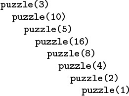
This nested sequence of function calls eventually terminates, but we cannot prove that the recursive function in Program 5.2 does not have arbitrarily deep nesting for some argument. We prefer recursive programs that always invoke themselves with smaller arguments.
Figure 5.1 Example of a recursive call chain
Program 5.3 is a compact implementation of Euclid’s algorithm for finding the greatest common divisor of two integers. It is based on the observation that the greatest common divisor of two integers x and y with x > y is the same as the greatest common divisor of y and x mod y (the remainder when x is divided by y). A number t divides both x and y if and only if t divides both y and x mod y, because x is equal to x mod y plus a multiple of y. The recursive calls made for an example invocation of this program are shown in Figure 5.2. For Euclid’s algorithm, the depth of the recursion depends on arithmetic properties of the arguments (it is known to be logarithmic).
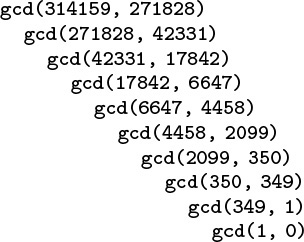
This nested sequence of function calls illustrates the operation of Euclid’s algorithm in discovering that 314159 and 271828 are relatively prime.
Figure 5.2 Example of Euclid’s algorithm
Program 5.4 is an example with multiple recursive calls. It is another expression evaluator, performing essentially the same computations as Program 4.2, but on prefix (rather than postfix) expressions, and letting recursion take the place of the explicit pushdown stack. In this chapter, we shall see many other examples of recursive programs and equivalent programs that use pushdown stacks. We shall examine the specific relationship between several pairs of such programs in detail.
Figure 5.3 shows the operation of Program 5.4 on a sample prefix expression. The multiple recursive calls mask a complex series of computations. Like most recursive programs, this program is best understood inductively: Assuming that it works properly for simple expressions, we can convince ourselves that it works properly for complex ones. This program is a simple example of a recursive descent parser—we can use the same process to convert C programs into machine code.

This nested sequence of function calls illustrates the operation of the recursive prefix-expression–evaluation algorithm on a sample expression. For simplicity, the expression arguments are shown here. The algorithm itself never explicitly decides the extent of its argument string: rather, it takes what it needs from the front of the string.
Figure 5.3 Prefix expression evaluation example
A precise inductive proof that Program 5.4 evaluates the expression properly is certainly much more challenging to write than are the proofs for functions with integer arguments that we have been discussing, and we shall encounter recursive programs and data structures that are even more complicated than this one throughout this book. Accordingly, we do not pursue the idealistic goal of providing complete inductive proofs of correctness for every recursive program that we write. In this case, the ability of the program to “know” how to separate the operands corresponding to a given operator seems mysterious at first (perhaps because we cannot immediately see how to do this separation at the top level), but is actually a straightforward calculation (because the path to pursue at each function call is unambiguously determined by the first character in the expression).
In principle, we can replace any for loop by an equivalent recursive program. Often, the recursive program is a more natural way to express the computation than the for loop, so we may as well take advantage of the mechanism provided by the programming system that supports recursion. There is one hidden cost, however, that we need to bear in mind. As is plain from the examples that we examined in Figures 5.1 through 5.3, when we execute a recursive program, we are nesting function calls, until we reach a point where we do not do a recursive call, and we return instead. In most programming environments, such nested function calls are implemented using the equivalent of built-in pushdown stacks. We shall examine the nature of such implementations throughout this chapter. The depth of the recursion is the maximum degree of nesting of the function calls over the course of the computation. Generally, the depth will depend on the input. For example, the depths of the recursions for the examples depicted in Figures 5.2 and 5.3 are 9 and 4, respectively. When using a recursive program, we need to take into account that the programming environment has to maintain a pushdown stack of size proportional to the depth of the recursion. For huge problems, the space needed for this stack might prevent us from using a recursive solution.
Data structures built from nodes with pointers are inherently recursive. For example, our definition of linked lists in Chapter 3 (Definition 3.3) is recursive. Therefore, recursive programs provide natural implementations of many commonly used functions for manipulating such data structures. Program 5.5 comprises four examples. We use such implementations frequently throughout the book, primarily because they are so much easier to understand than are their nonrecursive counterparts. However, we must exercise caution in using programs such as those in Program 5.5 when processing huge lists, because the depth of the recursion for those functions can be proportional to the length of the lists, so the space required for the recursive stack might become prohibitive.
Some programming environments automatically detect and eliminate tail recursion, when the last action of a function is a recursive call, because it is not strictly necessary to add to the depth of the recursion in such a case. This improvement would effectively transform the count, traversal, and deletion functions in Program 5.5 into loops, but it does not apply to the reverse-order traversal function.
In Sections 5.2 and 5.3, we consider two families of recursive algorithms that represent essential computational paradigms. Then, in Sections 5.4 through 5.7, we consider recursive data structures that serve as the basis for a very large fraction of the algorithms that we consider.
5.2 Modify Program 5.1 to compute N! mod M, such that overflow is no longer an issue. Try running your program for M = 997 and N = 103, 104, 105, and 106, to get an indication of how your programming system handles deeply nested recursive calls.
![]() 5.3 Give the sequences of argument values that result when Program 5.2 is invoked for each of the integers 1 through 9.
5.3 Give the sequences of argument values that result when Program 5.2 is invoked for each of the integers 1 through 9.
![]() 5.4 Find the value of N < 106 for which Program 5.2 makes the maximum number of recursive calls.
5.4 Find the value of N < 106 for which Program 5.2 makes the maximum number of recursive calls.
![]() 5.5 Provide a nonrecursive implementation of Euclid’s algorithm.
5.5 Provide a nonrecursive implementation of Euclid’s algorithm.
![]() 5.6 Give the figure corresponding to Figure 5.2 for the result of running Euclid’s algorithm for the inputs 89 and 55.
5.6 Give the figure corresponding to Figure 5.2 for the result of running Euclid’s algorithm for the inputs 89 and 55.
![]() 5.7 Give the recursive depth of Euclid’s algorithm when the input values are two consecutive Fibonacci numbers (FN and FN+1).
5.7 Give the recursive depth of Euclid’s algorithm when the input values are two consecutive Fibonacci numbers (FN and FN+1).
![]() 5.8 Give the figure corresponding to Figure 5.3 for the result of recursive prefix-expression evaluation for the input
5.8 Give the figure corresponding to Figure 5.3 for the result of recursive prefix-expression evaluation for the input + * * 12 12 12 144.
5.9 Write a recursive program to evaluate postfix expressions.
5.10 Write a recursive program to evaluate infix expressions. You may assume that operands are always enclosed in parentheses.
![]() 5.11 Write a recursive program that converts infix expressions to postfix.
5.11 Write a recursive program that converts infix expressions to postfix.
![]() 5.12 Write a recursive program that converts postfix expressions to infix.
5.12 Write a recursive program that converts postfix expressions to infix.
5.13 Write a recursive program for solving the Josephus problem (see Section 3.3).
5.14 Write a recursive program that deletes the final element of a linked list.
![]() 5.15 Write a recursive program for reversing the order of the nodes in a linked list (see Program 3.7). Hint: Use a global variable.
5.15 Write a recursive program for reversing the order of the nodes in a linked list (see Program 3.7). Hint: Use a global variable.
5.2 Divide and Conquer
Many of the recursive programs that we consider in this book use two recursive calls, each operating on about one-half of the input. This recursive scheme is perhaps the most important instance of the well-known divide-and-conquer paradigm for algorithm design, which serves as the basis for many of our most important algorithms.
As an example, let us consider the task of finding the maximum among N items stored in an array a[0], ..., a[N-1]. We can easily accomplish this task with a single pass through the array, as follows:
for (t = a[0], i = 1; i < N; i++)
if (a[i] > t) t = a[i];
The recursive divide-and-conquer solution given in Program 5.6 is also a simple (entirely different) algorithm for the same problem; we use it to illustrate the divide-and-conquer concept.
Most often, we use the divide-and-conquer approach because it provides solutions faster than those available with simple iterative algorithms (we shall discuss several examples at the end of this section), but it also is worthy of close examination as a way of understanding the nature of certain fundamental computations.
Figure 5.4 shows the recursive calls that are made when Program 5.6 is invoked for a sample array. The underlying structure seems complicated, but we normally do not need to worry about it—we depend on a proof by induction that the program works, and we use a recurrence relation to analyze the program’s performance.
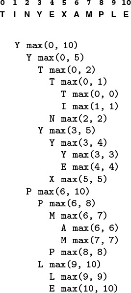
This sequence of function calls illustrates the dynamics of finding the maximum with a recursive algorithm.
Figure 5.4 A recursive approach to finding the maximum
As usual, the code itself suggests the proof by induction that it performs the desired computation:
• It finds the maximum for arrays of size 1 explicitly and immediately.
• For N > 1, it partitions the array into two arrays of size less than N, finds the maximum of the two parts by the inductive hypothesis, and returns the larger of these two values, which must be the maximum value in the whole array.
Moreover, we can use the recursive structure of the program to understand its performance characteristics.
Property 5.1 A recursive function that divides a problem of size N into two independent (nonempty) parts that it solves recursively calls itself less than N times.
If the parts are one of size k and one of size N – k, then the total number of recursive function calls that we use is
TN = Tk + TN – k + 1, for N ≥ 1 with T1 = 0.
The solution TN = N – 1 is immediate by induction. If the sizes sum to a value less than N, the proof that the number of calls is less than N – 1 follows the same inductive argument. We can prove analogous results under general conditions (see Exercise 5.20). ![]()
Program 5.6 is representative of many divide-and-conquer algorithms with precisely the same recursive structure, but other examples may differ in two primary respects. First, Program 5.6 does a constant amount of work on each function call, so its total running time is linear. Other divide-and-conquer algorithms may perform more work on each function call, as we shall see, so determining the total running time requires more intricate analysis. The running time of such algorithms depends on the precise manner of division into parts. Second, Program 5.6 is representative of divide-and-conquer algorithms for which the parts sum to make the whole. Other divide-and-conquer algorithms may divide into smaller parts that constitute less than the whole problem, or overlapping parts that total up to more than the whole problem. These algorithms are still proper recursive algorithms because each part is smaller than the whole, but analyzing them is more difficult than analyzing Program 5.6. We shall consider the analysis of these different types of algorithms in detail as we encounter them.
For example, the binary-search algorithm that we studied in Section 2.6 is a divide-and-conquer algorithm that divides a problem in half, then works on just one of the halves. We examine a recursive implementation of binary search in Chapter 12.
Figure 5.5 indicates the contents of the internal stack maintained by the programming environment to support the computation in Figure 5.4. The model depicted in the figure is idealistic, but it gives useful insights into the structure of the divide-and-conquer computation. If a program has two recursive calls, the actual internal stack contains one entry corresponding to the first function call while that function is being executed (which contains values of arguments, local variables, and a return address), then a similar entry corresponding to the second function call while that function is being executed. The alternative that is depicted in Figure 5.5 is to put the two entries on the stack at once, keeping all the subtasks remaining to be done explicitly on the stack. This arrangement plainly delineates the computation, and sets the stage for more general computational schemes, such as those that we examine in Sections 5.6 and 5.8.
This sequence is an idealistic representation of the contents of the internal stack during the sample computation of Figure 5.4. We start with the left and right indices of the whole subarray on the stack. Each line depicts the result of popping two indices and, if they are not equal, pushing four indices, which delimit the left subarray and the right subarray after the popped subarray is divided into two parts. In practice, the system keeps return addresses and local variables on the stack, instead of this specific representation of the work to be done, but this model suffices to describe the computation.
Figure 5.5 Example of internal stack dynamics
Figure 5.6 depicts the structure of the divide-and-conquer find-the-maximum computation. It is a recursive structure: the node at the top contains the size of the input array, the structure for the left subarray is drawn at the left and the structure for the right subarray is drawn at the right. We will formally define and discuss tree structures of this type in in Sections 5.4 and 5.5. They are useful for understanding the structure of any program involving nested function calls—recursive programs in particular. Also shown in Figure 5.6 is the same tree, but with each node labeled with the return value for the corresponding function call. In Section 5.7, we shall consider the process of building explicit linked structures that represent trees like this one.
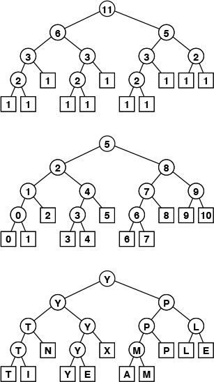
The divide-and-conquer algorithm splits a problem of size 11 into one of size 6 and one of size 5, a problem of size 6 into two problems of size 3, and so forth, until reaching problems of size 1 (top). Each circle in these diagrams represents a call on the recursive function, to the nodes just below connected to it by lines (squares are those calls for which the recursion terminates). The diagram in the middle shows the value of the index into the middle of the file that we use to effect the split; the diagram at the bottom shows the return value.
Figure 5.6 Recursive structure of find-the-maximum algorithm.
No discussion of recursion would be complete without the ancient towers of Hanoi problem. We have three pegs and N disks that fit onto the pegs. The disks differ in size, and are initially arranged on one of the pegs, in order from largest (disk N) at the bottom to smallest (disk 1) at the top. The task is to move the stack of disks to the right one position (peg), while obeying the following rules: (i) only one disk may be shifted at a time; and (ii) no disk may be placed on top of a smaller one. One legend says that the world will end when a certain group of monks accomplishes this task in a temple with 40 golden disks on three diamond pegs.
Program 5.7 gives a recursive solution to the problem. It specifies which disk should be shifted at each step, and in which direction (+ means move one peg to the right, cycling to the leftmost peg when on the rightmost peg; and - means move one peg to the left, cycling to the rightmost peg when on the leftmost peg). The recursion is based on the following idea: To move N disks one peg to the right, we first move the top N – 1 disks one peg to the left, then shift disk N one peg to the right, then move the N – 1 disks one more peg to the left (onto disk N). We can verify that this solution works by induction. Figure 5.7 shows the moves for N = 5 and the recursive calls for N = 3. An underlying pattern is evident, which we now consider in detail.
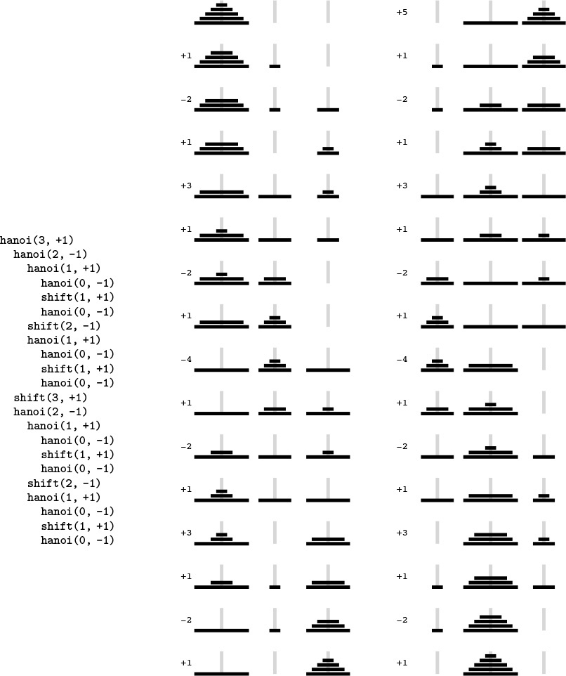
This diagram depicts the solution to the towers of Hanoi problem for five disks. We shift the top four disks left one position (left column), then move disk 5 to the right, then shift the top four disks left one position (right column). The sequence of function calls that follows constitutes the computation for three disks. The computed sequence of moves is +1 -2 +1 +3 +1 -2 +1, which appears four times in the solution (for example, the first seven moves).
Figure 5.7 Towers of Hanoi
First, the recursive structure of this solution immediately tells us the number of moves that the solution requires.
Property 5.2 The recursive divide-and-conquer algorithm for the towers of Hanoi problem produces a solution that has 2N – 1 moves.
As usual, it is immediate from the code that the number of moves satisfies a recurrence. In this case, the recurrence satisfied by the number of disk moves is similar to Formula 2.5:
TN = 2TN – 1 + 1, for N ≥ 2 with T1 = 1.
We can verify the stated result directly by induction: we have T (1) = 21 – 1 = 1; and, if T (k) = 2k – 1 for k < N, then T (N) = 2(2N – 1 – 1) + 1 = 2N – 1. ![]()
If the monks are moving disks at the rate of one per second, it will take at least 348 centuries for them to finish (see Figure 2.1), assuming that they do not make a mistake. The end of the world is likely be even further off than that because those monks presumably never have had the benefit of being able to use Program 5.7, and might not be able to figure out so quickly which disk to move next. We now consider an analysis of the method that leads to a simple (nonrecursive) method that makes the decision easy. While we may not wish to let the monks in on the secret, it is relevant to numerous important practical algorithms.
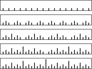
To understand the towers of Hanoi solution, let us consider the simple task of drawing the markings on a ruler. Each inch on the ruler has a mark at the 1/2 inch point, slightly shorter marks at 1/4 inch intervals, still shorter marks at 1/8 inch intervals, and so forth. Our task is to write a program to draw these marks at any given resolution, assuming that we have at our disposal a procedure mark(x, h) to make a mark h units high at position x.
If the desired resolution is 1/2n inches, we rescale so that our task is to put a mark at every point between 0 and 2n, endpoints not included. Thus, the middle mark should be n units high, the marks in the middle of the left and right halves should be n – 1 units high, and so forth. Program 5.8 is a straightforward divide-and-conquer algorithm to accomplish this objective; Figure 5.8 illustrates it in operation on a small example. Recursively speaking, the idea behind the method is the following. To make the marks in an interval, we first divide the interval into two equal halves. Then, we make the (shorter) marks in the left half (recursively), the long mark in the middle, and the (shorter) marks in the right half (recursively). Iteratively speaking, Figure 5.8 illustrates that the method makes the marks in order, from left to right—the trick lies in computing the lengths. The recursion tree in the figure helps us to understand the computation: Reading down, we see that the length of the mark decreases by 1 for each recursive function call. Reading across, we get the marks in the order that they are drawn, because, for any given node, we first draw the marks associated with the function call on the left, then the mark associated with the node, then the marks associated with the function call on the right.
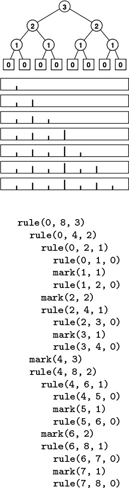
This sequence of function calls constitutes the computation for drawing a ruler of length 8, resulting in marks of lengths 1, 2, 1, 3, 1, 2, and 1.
Figure 5.8 Ruler-drawing function calls
We see immediately that the sequence of lengths is precisely the same as the sequence of disks moved for the towers of Hanoi problem. Indeed, a simple proof that they are identical is that the recursive programs are the same. Put another way, our monks could use the marks on a ruler to decide which disk to move.
Moreover, both the towers of Hanoi solution in Program 5.7 and the ruler-drawing program in Program 5.8 are variants of the basic divide-and-conquer scheme exemplified by Program 5.6. All three solve a problem of size 2n by dividing it into two problems of size 2n–1. For finding the maximum, we have a linear-time solution in the size of the input; for drawing a ruler and for solving the towers of Hanoi, we have a linear-time solution in the size of the output. For the towers of Hanoi, we normally think of the solution as being exponential time, because we measure the size of the problem in terms of the number of disks, n.
It is easy to draw the marks on a ruler with a recursive program, but is there some simpler way to compute the length of the ith mark, for any given i? Figure 5.9 shows yet another simple computational process that provides the answer to this question. The ith number printed out by both the towers of Hanoi program and the ruler program is nothing other than the number of trailing 0 bits in the binary representation of i. We can prove this property by induction by correspondence with a divide-and-conquer formulation for the process of printing the table of n-bit numbers: Print the table of (n – 1)-bit numbers, each preceded by a 0 bit, then print the table of (n – 1)-bit numbers each preceded by a 1-bit (see Exercise 5.25).
Computing the ruler function is equivalent to counting the number of trailing zeros in the even N-bit numbers.
Figure 5.9 Binary counting and the ruler function
For the towers of Hanoi problem, the implication of the correspondence with n-bit numbers is a simple algorithm for the task. We can move the pile one peg to the right by iterating the following two steps until done:
• Move the small disk to the right if n is odd (left if n is even).
• Make the only legal move not involving the small disk.
That is, after we move the small disk, the other two pegs contain two disks, one smaller than the other. The only legal move not involving the small disk is to move the smaller one onto the larger one. Every other move involves the small disk for the same reason that every other number is odd and that every other mark on the rule is the shortest. Perhaps our monks do know this secret, because it is hard to imagine how they might be deciding which moves to make otherwise.
A formal proof by induction that every other move in the towers of Hanoi solution involves the small disk (beginning and ending with such moves) is instructive: For n = 1, there is just one move, involving the small disk, so the property holds. For n > 1, the assumption that the property holds for n – 1 implies that it holds for n by the recursive construction: The first solution for n – 1 begins with a small-disk move, and the second solution for n – 1 ends with a small-disk move, so the solution for n begins and ends with a small-disk move. We put a move not involving the small disk in between two moves that do involve the small disk (the move ending the first solution for n – 1 and the move beginning the second solution for n – 1), so the property that every other move involves the small disk is preserved.
Program 5.9 is an alternate way to draw a ruler that is inspired by the correspondence to binary numbers (see Figure 5.10). We refer to this version of the algorithm as a bottom-up implementation. It is not recursive, but it is certainly suggested by the recursive algorithm. This correspondence between divide-and-conquer algorithms and the binary representations of numbers often provides insights for analysis and development of improved versions, such as bottom-up approaches. We consider this perspective to understand, and possibly to improve, each of the divide-and-conquer algorithms that we examine.
To draw a ruler nonrecursively, we alternate drawing marks of length 1 and skipping positions, then alternate drawing marks of length 2 and skipping remaining positions, then alternate drawing marks of length 3 and skipping remaining positions, and so forth.
Figure 5.10 Drawing a ruler in bottom-up order
The bottom-up approach involves rearranging the order of the computation when we are drawing a ruler. Figure 5.11 shows another example, where we rearrange the order of the three function calls in the recursive implementation. It reflects the recursive computation in the way that we first described it: Draw the middle mark, then draw the left half, then draw the right half. The pattern of drawing the marks is complex, but is the result of simply exchanging two statements in Program 5.8. As we shall see in Section 5.6, the relationship between Figures 5.8 and 5.11 is akin to the distinction between postfix and prefix in arithmetic expressions.

This sequence indicates the result of drawing marks before the recursive calls, instead of in between them.
Figure 5.11 Ruler-drawing function calls (preorder version)
Drawing the marks in order as in Figure 5.8 might be preferable to doing the rearranged computations contained in Program 5.9 and indicated in Figure 5.11, because we can draw an arbitrarily long ruler, if we imagine a drawing device that simply moves on to the next mark in a continuous scroll. Similarly, to solve the towers of Hanoi problem, we are constrained to produce the sequence of disk moves in the order that they are to be performed. In general, many recursive programs depend on the subproblems being solved in a particular order. For other computations (see, for example, Program 5.6), the order in which we solve the subproblems is irrelevant. For such computations, the only constraint is that we must solve the subproblems before we can solve the main problem. Understanding when we have the flexibility to reorder the computation not only is a secret to success in algorithm design, but also has direct practical effects in many contexts. For example, this matter is critical when we consider implementing algorithms on parallel processors.
The bottom-up approach corresponds to the general method of algorithm design where we solve a problem by first solving trivial subproblems, then combining those solutions to solve slightly bigger subproblems, and so forth, until the whole problem is solved. This approach might be called combine and conquer.
It is a small step from drawing rulers to drawing two-dimensional patterns such as Figure 5.12. This figure illustrates how a simple recursive description can lead to a computation that appears to be complex (see Exercise 5.30).
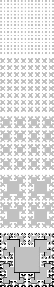
This fractal is a two-dimensional version of Figure 5.10. The outlined boxes in the bottom diagram highlight the recursive structure of the computation.
Figure 5.12 Two-dimensional fractal star
Recursively defined geometric patterns such as Figure 5.12 are sometimes called fractals. If more complicated drawing primitives are used, and more complicated recursive invocations are involved (especially including recursively-defined functions on reals and in the complex plane), patterns of remarkable diversity and complexity can be developed. Another example, demonstrated in Figure 5.13, is the Koch star, which is defined recursively as follows: A Koch star of order 0 is the simple hill example of Figure 4.3, and a Koch star of order n is a Koch star of order n – 1 with each line segment replaced by the star of order 0, scaled appropriately.

This modification to the PostScript program of Figure 4.3 transforms the output into a fractal (see text).
Figure 5.13 Recursive PostScript for Koch fractal
Like the ruler-drawing and the towers of Hanoi solutions, these algorithms are linear in the number of steps, but that number is exponential in the maximum depth of the recursion (see Exercises 5.29 and 5.33). They also can be directly related to counting in an appropriate number system (see Exercise 5.34).
The towers of Hanoi problem, ruler-drawing problem, and fractals are amusing; and the connection to binary numbers is surprising, but our primary interest in all of these topics is that they provide us with insights in understanding the basic algorithm design paradigm of divide in half and solve one or both halves independently, which is perhaps the most important such technique that we consider in this book. Table 5.1 includes details about binary search and mergesort, which not only are important and widely used practical algorithms, but also exemplify the divide-and-conquer algorithm design paradigm.
Binary search (see Chapters 2 and 12) and mergesort (see Chapter 8) are prototypical divide-and-conquer algorithms that provide guaranteed optimal performance for searching and sorting, respectively. The recurrences indicate the nature of the divide-and-conquer computation for each algorithm. (See Sections 2.5 and 2.6 for derivations of the solutions in the rightmost column.) Binary search splits a problem in half, does 1 comparison, then makes a recursive call for one of the halves. Mergesort splits a problem in half, then works on both halves recursively, then does N comparisons. Throughout the book, we shall consider numerous other algorithms developed with these recursive schemes.
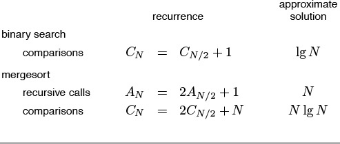
Table 5.1 Basic divide-and-conquer algorithms
Quicksort (see Chapter 7) and binary-tree search (see Chapter 12) represent a significant variation on the basic divide-and-conquer theme where the problem is split into subproblems of size k – 1 and N – k, for some value k, which is determined by the input. For random input, these algorithms divide a problem into subproblems that are half the size (as in mergesort or in binary search) on the average. We study the analysis of the effects of this difference when we discuss these algorithms.
Other variations on the basic theme that are worthy of consideration include these: divide into parts of varying size, divide into more than two parts, divide into overlapping parts, and do various amounts of work in the nonrecursive part of the algorithm. In general, divide-and-conquer algorithms involve doing work to split the input into pieces, or to merge the results of processing two independent solved portions of the input, or to help things along after half of the input has been processed. That is, there may be code before, after, or in between the two recursive calls. Naturally, such variations lead to algorithms more complicated than are binary search and mergesort, and are more difficult to analyze. We consider numerous examples in this book; we return to advanced applications and analysis in Part 8.
Exercises
5.16 Write a recursive program that finds the maximum element in an array, based on comparing the first element in the array against the maximum element in the rest of the array (computed recursively).
5.17 Write a recursive program that finds the maximum element in a linked list.
5.18 Modify the divide-and-conquer program for finding the maximum element in an array (Program 5.6) to divide an array of size N into one part of size k = 2![]() lg N
lg N![]() – 1 and another of size N – k (so that the size of at least one of the parts is a power of 2).
– 1 and another of size N – k (so that the size of at least one of the parts is a power of 2).
5.19 Draw the tree corresponding to the recursive calls that your program from Exercise 5.18 makes when the array size is 11.
![]() 5.20 Prove by induction that the number of function calls made by any divide-and-conquer algorithm that divides a problem into parts that constitute the whole, then solves the parts recursively, is linear.
5.20 Prove by induction that the number of function calls made by any divide-and-conquer algorithm that divides a problem into parts that constitute the whole, then solves the parts recursively, is linear.
![]() 5.21 Prove that the recursive solution to the towers of Hanoi problem (Program 5.7) is optimal. That is, show that any solution requires at least 2N – 1 moves.
5.21 Prove that the recursive solution to the towers of Hanoi problem (Program 5.7) is optimal. That is, show that any solution requires at least 2N – 1 moves.
![]() 5.22 Write a recursive program that computes the length of the ith mark in a ruler with 2n – 1 marks.
5.22 Write a recursive program that computes the length of the ith mark in a ruler with 2n – 1 marks.
![]() 5.23 Examine tables of n-bit numbers, such as Figure 5.9, to discover a property of the ith number that determines the direction of the ith move (indicated by the sign bit in Figure 5.7) for solving the towers of Hanoi problem.
5.23 Examine tables of n-bit numbers, such as Figure 5.9, to discover a property of the ith number that determines the direction of the ith move (indicated by the sign bit in Figure 5.7) for solving the towers of Hanoi problem.
5.24 Write a program that produces a solution to the towers of Hanoi problem by filling in an array that holds all the moves, as in Program 5.9.
![]() 5.25 Write a recursive program that fills in an n-by-2n array with 0s and 1s such that the array represents all the n-bit binary numbers, as depicted in Figure 5.9.
5.25 Write a recursive program that fills in an n-by-2n array with 0s and 1s such that the array represents all the n-bit binary numbers, as depicted in Figure 5.9.
5.26 Draw the results of using the recursive ruler-drawing program (Program 5.8) for these unintended values of the arguments: rule(0, 11, 4), rule(4, 20, 4), and rule(7, 30, 5).
5.27 Prove the following fact about the ruler-drawing program (Program 5.8): If the difference between its first two arguments is a power of 2, then both of its recursive calls have this property also.
![]() 5.28 Write a function that computes efficiently the number of trailing 0s in the binary representation of an integer.
5.28 Write a function that computes efficiently the number of trailing 0s in the binary representation of an integer.
![]() 5.29 How many squares are there in Figure 5.12 (counting the ones that are covered up by bigger squares)?
5.29 How many squares are there in Figure 5.12 (counting the ones that are covered up by bigger squares)?
![]() 5.30 Write a recursive C program that outputs a PostScript program that draws the bottom diagram in Figure 5.12, in the form of a list of function calls
5.30 Write a recursive C program that outputs a PostScript program that draws the bottom diagram in Figure 5.12, in the form of a list of function calls x y r box, which draws an r-by-r square at (x, y). Implement box in PostScript (see Section 4.3).
5.31 Write a bottom-up nonrecursive program (similar to Program 5.9) that draws the bottom diagram in Figure 5.12, in the manner described in Exercise 5.30.
![]() 5.32 Write a PostScript program that draws the bottom diagram in Figure 5.12.
5.32 Write a PostScript program that draws the bottom diagram in Figure 5.12.
![]() 5.33 How many line segments are there in a Koch star of order n?
5.33 How many line segments are there in a Koch star of order n?
![]() 5.34 Drawing a Koch star of order n amounts to executing a sequence of commands of the form “rotate α degrees, then draw a line segment of length 1/3n.” Find a correspondence with number systems that gives you a way to draw the star by incrementing a counter, then computing the angle α from the counter value.
5.34 Drawing a Koch star of order n amounts to executing a sequence of commands of the form “rotate α degrees, then draw a line segment of length 1/3n.” Find a correspondence with number systems that gives you a way to draw the star by incrementing a counter, then computing the angle α from the counter value.
![]() 5.35 Modify the Koch star program in Figure 5.13 to produce a different fractal based on a five-line figure for order 0, defined by 1-unit moves east, north, east, south, and east, in that order (see Figure 4.3).
5.35 Modify the Koch star program in Figure 5.13 to produce a different fractal based on a five-line figure for order 0, defined by 1-unit moves east, north, east, south, and east, in that order (see Figure 4.3).
5.36 Write a recursive divide-and-conquer function to draw an approximation to a line segment in an integer coordinate space, given the endpoints. Assume that all coordinates are between 0 and M. Hint: First plot a point close to the middle.
5.3 Dynamic Programming
An essential characteristic of the divide-and-conquer algorithms that we considered in Section 5.2 is that they partition the problem into independent subproblems. When the subproblems are not independent, the situation is more complicated, primarily because direct recursive implementations of even the simplest algorithms of this type can require unthinkable amounts of time. In this section, we consider a systematic technique for avoiding this pitfall for an important class of problems.
For example, Program 5.10 is a direct recursive implementation of the recurrence that defines the Fibonacci numbers (see Section 2.3). Do not use this program: It is spectacularly inefficient. Indeed, the number of recursive calls to compute FN is exactly FN+1. But FN is about φN, where φ ≈ 1.618 is the golden ratio. The awful truth is that Program 5.10 is an exponential-time algorithm for this trivial computation. Figure 5.14, which depicts the recursive calls for a small example, makes plain the amount of recomputation that is involved.

The picture of the recursive calls needed to used to compute F8 by the standard recursive algorithm illustrates how recursion with overlapping subproblems can lead to exponential costs. In this case, the second recursive call ignores the computations done during the first, which results in massive recomputation because the effect multiplies recursively. The recursive calls to compute F6 = 8 (which are reflected in the right subtree of the root and the left subtree of the left subtree of the root) are listed below.
Figure 5.14 Structure of recursive algorithm for Fibonacci numbers
By contrast, it is easy to compute FN in linear (proportional to N) time, by computing the first N Fibonacci numbers and storing them in an array:
F[0] = 0; F[1] = 1;
for (i = 2; i <= N; i++)
F[i] = F[i-1] + F[i-2];
The numbers grow exponentially, so the array is small—for example, F45 = 1836311903 is the largest Fibonacci number that can be represented as a 32-bit integer, so an array of size 46 will do.
This technique gives us an immediate way to get numerical solutions for any recurrence relation. In the case of Fibonacci numbers, we can even dispense with the array, and keep track of just the previous two values (see Exercise 5.37); for many other commonly encountered recurrences (see, for example, Exercise 5.40), we need to maintain the array with all the known values.
A recurrence is a recursive function with integer values. Our discussion in the previous paragraph leads to the conclusion that we can evaluate any such function by computing all the function values in order starting at the smallest, using previously computed values at each step to compute the current value. We refer to this technique as bottom-up dynamic programming. It applies to any recursive computation, provided that we can afford to save all the previously computed values. It is an algorithm-design technique that has been used successfully for a wide range of problems. We have to pay attention to a simple technique that can improve the running time of an algorithm from exponential to linear!
Top-down dynamic programming is an even simpler view of the technique that allows us to execute recursive functions at the same cost as (or less cost than) bottom-up dynamic programming, in an automatic way. We instrument the recursive program to save each value that it computes (as its final action), and to check the saved values to avoid recomputing any of them (as its first action). Program 5.11 is the mechanical transformation of Program 5.10 that reduces its running time to be linear via top-down dynamic programming. Figure 5.15 shows the drastic reduction in the number of recursive calls achieved by this simple automatic change. Top-down dynamic programming is also sometimes called memoization.

This picture of the recursive calls used to compute F8 by the top-down dynamic programming implementation of the recursive algorithm illustrates how saving computed values cuts the cost from exponential (see Figure 5.14) to linear.
Figure 5.15 Top-down dynamic programming for computing Fibonacci numbers
For a more complicated example, consider the knapsack problem: A thief robbing a safe finds it filled with N types of items of varying size and value, but has only a small knapsack of capacity M to use to carry the goods. The knapsack problem is to find the combination of items which the thief should choose for the knapsack in order to maximize the total value of all the stolen items. For example, with the item types depicted in Figure 5.16, a thief with a knapsack of size 17 can take five A’s (but not six) for a total take of 20, or a D and an E for a total take of 24, or one of many other combinations. Our goal is to find an efficient algorithm that somehow finds the maximum among all the possibilities, given any set of items and knapsack capacity.
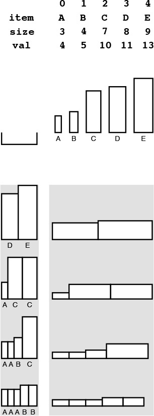
An instance of the knapsack problem (top) consists of a knapsack capacity and a set of items of varying size (horizontal dimension) and value (vertical dimension). This figure shows four different ways to fill a knapsack of size 17, two of which lead to the highest possible total value of 24.
Figure 5.16 Knapsack example
There are many applications in which solutions to the knapsack problem are important. For example, a shipping company might wish to know the best way to load a truck or cargo plane with items for shipment. In such applications, other variants to the problem might arise as well: for example, there might be a limited number of each kind of item available, or there might be two trucks. Many such variants can be handled with the same approach that we are about to examine for solving the basic problem just stated; others turn out to be much more difficult. There is a fine line between feasible and infeasible problems of this type, which we shall examine in Part 8.
In a recursive solution to the knapsack problem, each time that we choose an item, we assume that we can (recursively) find an optimal way to pack the rest of the knapsack. For a knapsack of size cap, we determine, for each item i among the available item types, what total value we could carry by placing i in the knapsack with an optimal packing of other items around it. That optimal packing is simply the one we have discovered (or will discover) for the smaller knapsack of size cap-items[i].size. This solution exploits the principle that optimal decisions, once made, do not need to be changed. Once we know how to pack knapsacks of smaller capacities with optimal sets of items, we do not need to reexamine those problems, regardless of what the next items are.
Program 5.12 is a direct recursive solution based on this discussion. Again, this program is not feasible for use in solving actual problems, because it takes exponential time due to massive recomputation (see Figure 5.17), but we can automatically apply top-down dynamic programming to eliminate this problem, as shown in Program 5.13. As before, this technique eliminates all recomputation, as shown in Figure 5.18.
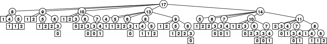
This tree represents the recursive call structure of the simple recursive knapsack algorithm in Program 5.12. The number in each node represents the remaining capacity in the knapsack. The algorithm suffers the same basic problem of exponential performance due to massive recomputation for overlapping subproblems that we considered in computing Fibonacci numbers (see Figure 5.14).
Figure 5.17 Recursive structure of knapsack algorithm.
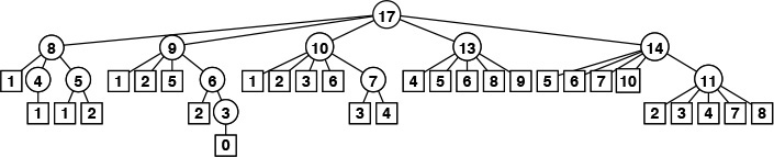
As it did for the Fibonacci numbers computation, the technique of saving known values reduces the cost of the knapsack algorithm from exponential (see Figure 5.17) to linear.
Figure 5.18 Top-down dynamic programming for knapsack algorithm
By design, dynamic programming eliminates all recomputation in any recursive program, subject only to the condition that we can afford to save the values of the function for arguments smaller than the call in question.
Property 5.3 Dynamic programming reduces the running time of a recursive function to be at most the time required to evaluate the function for all arguments less than or equal to the given argument, treating the cost of a recursive call as constant.
See Exercise 5.50. ![]()
For the knapsack problem, this property implies that the running time is proportional to NM. Thus, we can solve the knapsack problem easily when the capacity is not huge; for huge capacities, the time and space requirements may be prohibitively large.
Bottom-up dynamic programming applies to the knapsack problem, as well. Indeed, we can use the bottom-up approach any time that we use the top-down approach, although we need to take care to ensure that we compute the function values in an appropriate order, so that each value that we need has been computed when we need it. For functions with single integer arguments such as the two that we have considered, we simply proceed in increasing order of the argument (see Exercise 5.53); for more complicated recursive functions, determining a proper order can be a challenge.
For example, we do not need to restrict ourselves to recursive functions with single integer arguments. When we have a function with multiple integer arguments, we can save solutions to smaller subproblems in multidimensional arrays, one for each argument. Other situations involve no integer arguments at all, but rather use an abstract discrete problem formulation that allows us to decompose problems into smaller ones. We shall consider examples of such problems in Parts 5 through 8.
In top-down dynamic programming, we save known values; in bottom-up dynamic programming, we precompute them. We generally prefer top-down to bottom-up dynamic programming, because
• It is a mechanical transformation of a natural problem solution.
• The order of computing the subproblems takes care of itself.
• We may not need to compute answers to all the subproblems.
Dynamic-programming applications differ in the nature of the subproblems and in the amount of information that we need to save regarding the subproblems.
A crucial point that we cannot overlook is that dynamic programming becomes ineffective when the number of possible function values that we might need is so high that we cannot afford to save (top-down) or precompute (bottom-up) all of them. For example, if M and the item sizes are 64-bit quantities or floating-point numbers in the knapsack problem, we will not be able to save values by indexing into an array. This distinction causes more than a minor annoyance—it poses a fundamental difficulty. No good solution is known for such problems; we will see in Part 8 that there is good reason to believe that no good solution exists.
Dynamic programming is an algorithm-design technique that is primarily suited for the advanced problems of the type that we shall consider in Parts 5 through 8. Most of the algorithms that we discuss in Parts 2 through 4 are divide-and-conquer methods with nonoverlapping subproblems, and we are focusing on subquadratic or sublinear, rather than subexponential, performance. However, top-down dynamic programming is a basic technique for developing efficient implementations of recursive algorithms that belongs in the toolbox of anyone engaged in algorithm design and implementation.
Exercises
![]() 5.37 Write a function that computes FN mod M, using only a constant amount of space for intermediate calculations.
5.37 Write a function that computes FN mod M, using only a constant amount of space for intermediate calculations.
5.38 What is the largest N for which FN can be represented as a 64-bit integer?
![]() 5.39 Draw the tree corresponding to Figure 5.15 for the case where we exchange the recursive calls in Program 5.11.
5.39 Draw the tree corresponding to Figure 5.15 for the case where we exchange the recursive calls in Program 5.11.
5.40 Write a function that uses bottom-up dynamic programming to compute the value of PN defined by the recurrence
PN = ![]() N/2
N/2![]() + P
+ P![]() N/2
N/2![]() + P
+ P![]() N/2
N/2 ![]() , for N ≥ 1 with P0 = 0.
, for N ≥ 1 with P0 = 0.
Draw a plot of N versus PN – N lg N/2 for 0 ≤ N ≤ 1024.
5.41 Write a function that uses top-down dynamic programming to solve Exercise 5.40.
![]() 5.42 Draw the tree corresponding to Figure 5.15 for your function from Exercise 5.41, when invoked for N = 23.
5.42 Draw the tree corresponding to Figure 5.15 for your function from Exercise 5.41, when invoked for N = 23.
5.43 Draw a plot of N versus the number of recursive calls that your function from Exercise 5.41 makes to compute PN, for 0 ≤ N ≤ 1024. (For the purposes of this calculation, start your program from scratch for each N.)
5.44 Write a function that uses bottom-up dynamic programming to compute the value of CN defined by the recurrence
5.45 Write a function that uses top-down dynamic programming to solve Exercise 5.44.
![]() 5.46 Draw the tree corresponding to Figure 5.15 for your function from Exercise 5.45, when invoked for N = 23.
5.46 Draw the tree corresponding to Figure 5.15 for your function from Exercise 5.45, when invoked for N = 23.
5.47 Draw a plot of N versus the number of recursive calls that your function from Exercise 5.45 makes to compute CN, for 0 ≤ N ≤ 1024. (For the purposes of this calculation, start your program from scratch for each N.)
![]() 5.48 Give the contents of the arrays
5.48 Give the contents of the arrays maxKnown and itemKnown that are computed by Program 5.13 for the call knap(17) with the items in Figure 5.16.
![]() 5.49 Give the tree corresponding to Figure 5.18 under the assumption that the items are considered in decreasing order of their size.
5.49 Give the tree corresponding to Figure 5.18 under the assumption that the items are considered in decreasing order of their size.
![]() 5.50 Prove Property 5.3.
5.50 Prove Property 5.3.
![]() 5.51 Write a function that solves the knapsack problem using a bottom-up dynamic programming version of Program 5.12.
5.51 Write a function that solves the knapsack problem using a bottom-up dynamic programming version of Program 5.12.
![]() 5.52 Write a function that solves the knapsack problem using top-down dynamic programming, but using a recursive solution based on computing the optimal number of a particular item to include in the knapsack, based on (recursively) knowing the optimal way to pack the knapsack without that item.
5.52 Write a function that solves the knapsack problem using top-down dynamic programming, but using a recursive solution based on computing the optimal number of a particular item to include in the knapsack, based on (recursively) knowing the optimal way to pack the knapsack without that item.
![]() 5.53 Write a function that solves the knapsack problem using a bottom-up dynamic programming version of the recursive solution described in Exercise 5.52.
5.53 Write a function that solves the knapsack problem using a bottom-up dynamic programming version of the recursive solution described in Exercise 5.52.
![]() 5.54 Use dynamic programming to solve Exercise 5.4. Keep track of the total number of function calls that you save.
5.54 Use dynamic programming to solve Exercise 5.4. Keep track of the total number of function calls that you save.
5.55 Write a program that uses top-down dynamic programming to compute the binomial coefficient ![]() , based on the recursive rule
, based on the recursive rule
with ![]() .
.
5.4 Trees
Trees are a mathematical abstraction that play a central role in the design and analysis of algorithms because
• We use trees to describe dynamic properties of algorithms.
• We build and use explicit data structures that are concrete realizations of trees.
We have already seen examples of both of these uses. We designed algorithms for the connectivity problem that are based on tree structures in Chapter 1, and we described the call structure of recursive algorithms with tree structures in Sections 5.2 and 5.3.
We encounter trees frequently in everyday life—the basic concept is a familiar one. For example, many people keep track of ancestors or descendants with a family tree; as we shall see, much of our terminology is derived from this usage. Another example is found in the organization of sports tournaments; this usage was studied by Lewis Carroll, among others. A third example is found in the organizational chart of a large corporation; this usage is suggestive of the hierarchical decomposition that characterizes divide-and-conquer algorithms. A fourth example is a parse tree of an English sentence into its constituent parts; such trees are intimately related to the processing of computer languages, as discussed in Part 5. Figure 5.19 gives a typical example of a tree—one that describes the structure of this book. We touch on numerous other examples of applications of trees throughout the book.

This tree depicts the parts, chapters, and sections in this book. There is a node for each entity. Each node is connected to its constituent parts by links down to them, and is connected to the large part to which it belongs by a link up to that part.
Figure 5.19 A tree
In computer applications, one of the most familiar uses of tree structures is to organize file systems. We keep files in directories (which are also sometimes called folders) that are defined recursively as sequences of directories and files. This recursive definition again reflects a natural recursive decomposition, and is identical to the definition of a certain type of tree.
There are many different types of trees, and it is important to understand the distinction between the abstraction and the concrete representation with which we are working for a given application. Accordingly, we shall consider the different types of trees and their representations in detail. We begin our discussion by defining trees as abstract objects, and by introducing most of the basic associated terminology. We shall discuss informally the different types of trees that we need to consider in decreasing order of generality:
• Trees
• Rooted trees
• Ordered trees
• M-ary trees and binary trees
After developing a context with this informal discussion, we move to formal definitions and consider representations and applications. Figure 5.20 illustrates many of the basic concepts that we discuss and then define.
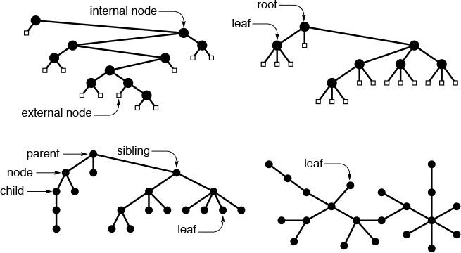
These diagrams show examples of a binary tree (top left), a ternary tree (top right), a rooted tree (bottom left), and a free tree (bottom right).
Figure 5.20 Types of trees
A tree is a nonempty collection of vertices and edges that satisfies certain requirements. A vertex is a simple object (also referred to as a node) that can have a name and can carry other associated information; an edge is a connection between two vertices. A path in a tree is a list of distinct vertices in which successive vertices are connected by edges in the tree. The defining property of a tree is that there is precisely one path connecting any two nodes. If there is more than one path between some pair of nodes, or if there is no path between some pair of nodes, then we have a graph; we do not have a tree. A disjoint set of trees is called a forest.
A rooted tree is one where we designate one node as the root of a tree. In computer science, we normally reserve the term tree to refer to rooted trees, and use the term free tree to refer to the more general structure described in the previous paragraph. In a rooted tree, any node is the root of a subtree consisting of it and the nodes below it.
There is exactly one path between the root and each of the other nodes in the tree. The definition implies no direction on the edges; we normally think of the edges as all pointing away from the root or all pointing towards the root, depending upon the application. We usually draw rooted trees with the root at the top (even though this convention seems unnatural at first), and we speak of node y as being below node x (and x as above y) if x is on the path from y to the root (that is, if y is below x as drawn on the page and is connected to x by a path that does not pass through the root). Each node (except the root) has exactly one node above it, which is called its parent; the nodes directly below a node are called its children. We sometimes carry the analogy to family trees further and refer to the grandparent or the sibling of a node.
Nodes with no children are called leaves, or terminal nodes. To correspond to the latter usage, nodes with at least one child are sometimes called nonterminal nodes. We have seen an example in this chapter of the utility of distinguishing these types of nodes. In trees that we use to present the call structure of recursive algorithms (see, for example, Figure 5.14) the nonterminal nodes (circles) represent function invocations with recursive calls and the terminal nodes (squares) represent function invocations with no recursive calls.
In certain applications, the way in which the children of each node are ordered is significant; in other applications, it is not. An ordered tree is a rooted tree in which the order of the children at every node is specified. Ordered trees are a natural representation: for example, we place the children in some order when we draw a tree. As we shall see, this distinction is also significant when we consider representing trees in a computer.
If each node must have a specific number of children appearing in a specific order, then we have an M-ary tree. In such a tree, it is often appropriate to define special external nodes that have no children. Then, external nodes can act as dummy nodes for reference by nodes that do not have the specified number of children. In particular, the simplest type of M-ary tree is the binary tree. A binary tree is an ordered tree consisting of two types of nodes: external nodes with no children and internal nodes with exactly two children. Since the two children of each internal node are ordered, we refer to the left child and the right child of internal nodes: every internal node must have both a left and a right child, although one or both of them might be an external node. A leaf in an M-ary tree is an internal node whose children are all external.
That is the basic terminology. Next, we shall consider formal definitions, representations, and applications of, in increasing order of generality,
• Binary trees and M-ary trees
• Ordered trees
• Rooted trees
• Free trees
That is, a binary tree is a special type of ordered tree, an ordered tree is a special type of rooted tree, and a rooted tree is a special type of free tree. The different types of trees arise naturally in various applications, and is important to be aware of the distinctions when we consider ways of representing trees with concrete data structures. By starting with the most specific abstract structure, we shall be able to consider concrete representations in detail, as will become clear.
Definition 5.1 A binary tree is either an external node or an internal node connected to a pair of binary trees, which are called the left subtree and the right subtree of that node.
This definition makes it plain that the binary tree itself is an abstract mathematical concept. When we are working with a computer representation, we are working with just one concrete realization of that abstraction. The situation is no different from representing real numbers with floats, integers with ints, and so forth. When we draw a tree with a node at the root connected by edges to the left subtree on the left and the right subtree on the right, we are choosing a convenient concrete representation. There are many different ways to represent binary trees (see, for example, Exercise 5.62) that are surprising at first, but, upon reflection, that are to be expected, given the abstract nature of the definition.
The concrete representation that we use most often when we implement programs that use and manipulate binary trees is a structure with two links (a left link and a right link) for internal nodes (see Figure 5.21). These structures are similar to linked lists, but they have two links per node, rather than one. Null links correspond to external nodes. Specifically, we add a link to our standard linked list representation from Section 3.3, as follows:
typedef struct node *link;
struct node { Item item; link l, r; };
The standard representation of a binary tree uses nodes with two links: a left link to the left subtree and a right link to the right subtree. Null links correspond to external nodes.
Figure 5.21 Binary-tree representation
which is nothing more than C code for Definition 5.1. Links are references to nodes, and a node consists of an item and a pair of links. Thus, for example, we implement the abstract operation move to the left subtree with a pointer reference such as x = x->l.
This standard representation allows for efficient implementation of operations that call for moving down the tree from the root, but not for operations that call for moving up the tree from a child to its parent. For algorithms that require such operations, we might add a third link to each node, pointing to the parent. This alternative is analogous to a doubly linked list. As with linked lists (see Figure 3.6), we keep tree nodes in an array and use indices instead of pointers as links in certain situations. We examine a specific instance of such an implementation in Section 12.7. We use other binary-tree representations for certain specific algorithms, most notably in Chapter 9.
Because of all the different possible representations, we might develop a binary-tree ADT that encapsulates the important operations that we want to perform, and that separates the use and implementation of these operations. We do not take this approach in this book because
• We most often use the two-link representation.
• We use trees to implement higher-level ADTs, and wish to focus on those.
• We work with algorithms whose efficiency depends on a particular representation—a fact that might be lost in an ADT.
These are the same reasons that we use familiar concrete representations for arrays and linked lists. The binary-tree representation depicted in Figure 5.21 is a fundamental tool that we are now adding to this short list.
For linked lists, we began by considering elementary operations for inserting and deleting nodes (see Figures 3.3 and 3.4). For the standard representation of binary trees, such operations are not necessarily elementary, because of the second link. If we want to delete a node from a binary tree, we have to reconcile the basic problem that we may have two children to handle after the node is gone, but only one parent. There are three natural operations that do not have this difficulty: insert a new node at the bottom (replace a null link with a link to a new node), delete a leaf (replace the link to it by a null link), and combine two trees by creating a new root with a left link pointing to one tree and the right link pointing to the other one. We use these operations extensively when manipulating binary trees.
Definition 5.2 An M-ary tree is either an external node or an internal node connected to an ordered sequence of M trees that are also M-ary trees.
We normally represent nodes in M-ary trees either as structures with M named links (as in binary trees) or as arrays of M links. For example, in Chapter 15, we consider 3-ary (or ternary) trees where we use structures with three named links (left, middle, and right) each of which has specific meaning for associated algorithms. Otherwise, the use of arrays to hold the links is appropriate because the value of M is fixed, although, as we shall see, we have to pay particular attention to excessive use of space when using such a representation.
Definition 5.3 A tree (also called an ordered tree) is a node (called the root) connected to a sequence of disjoint trees. Such a sequence is called a forest.
The distinction between ordered trees and M-ary trees is that nodes in ordered trees can have any number of children, whereas nodes in M-ary trees must have precisely M children. We sometimes use the term general tree in contexts where we want to distinguish ordered trees from M-ary trees.
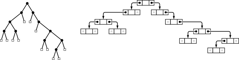
Because each node in an ordered tree can have any number of links, it is natural to consider using a linked list, rather than an array, to hold the links to the node’s children. Figure 5.22 is an example of such a representation. From this example, it is clear that each node then contains two links, one for the linked list connecting it to its siblings, the other for the linked list of its children.
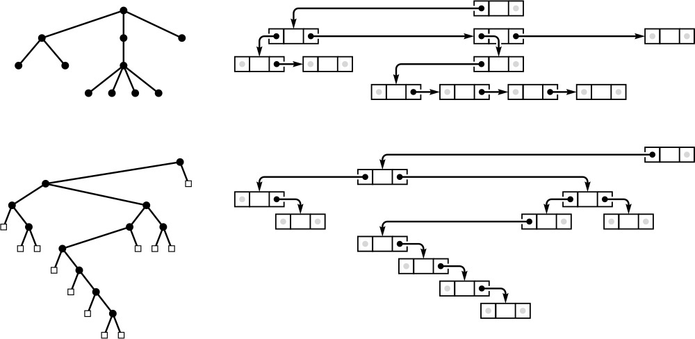
Representing an ordered tree by keeping a linked list of the children of each node is equivalent to representing it as a binary tree. The diagram on the right at the top shows a linked-list-of-children representation of the tree on the left at the top, with the list implemented in the right links of nodes, and each node’s left link pointing to the first node in the linked list of its children. The diagram on the right at the bottom shows a slightly rearranged version of the diagram above it, and clearly represents the binary tree at the left on the bottom. That is, we can consider the binary tree as representing the tree.
Figure 5.22 Tree representation
Property 5.4 There is a one-to-one correspondence between binary trees and ordered forests.
The correspondence is depicted in Figure 5.22. We can represent any forest as a binary tree by making the left link of each node point to its leftmost child, and the right link of each node point to its sibling on the right. ![]()
Definition 5.4 A rooted tree (or unordered tree) is a node (called the root) connected to a multiset of rooted trees. (Such a multiset is called an unordered forest.)
The trees that we encountered in Chapter 1 for the connectivity problem are unordered trees. Such trees may be defined as ordered trees where the order in which the children of a node are considered is not significant. We could also choose to define unordered trees as comprising a set of parent–child relationships among nodes. This choice would seem to have little relation to the recursive structures that we are considering, but it is perhaps the concrete representation that is most true to the abstract notion.
We could choose to represent an unordered tree in a computer with an ordered tree, recognizing that many different ordered trees might represent the same unordered tree. Indeed, the converse problem of determining whether or not two different ordered trees represent the same unordered tree (the tree-isomorphism problem) is a difficult one to solve.
The most general type of tree is one where no root node is distinguished. For example, the spanning trees resulting from the connectivity algorithms in Chapter 1 have this property. To define properly unrooted, unordered trees, or free trees, we start with a definition for graphs.
Definition 5.5 A graph is a set of nodes together with a set of edges that connect pairs of distinct nodes (with at most one edge connecting any pair of nodes).
We can envision starting at some node and following an edge to the constituent node for the edge, then following an edge from that node to another node, and so on. A sequence of edges leading from one node to another in this way with no node appearing twice is called a simple path. A graph is connected if there is a simple path connecting any pair of nodes. A path that is simple except that the first and final nodes are the same is called a cycle.
Every tree is a graph; which graphs are trees? We consider a graph to be a tree if it satisfies any of the following four conditions:
• G has N – 1 edges and no cycles.
• G has N – 1 edges and is connected.
• Exactly one simple path connects each pair of vertices in G.
• G is connected, but does not remain connected if any edge is removed.
Any one of these conditions is necessary and sufficient to prove the other three. Formally, we should choose one of them to serve as a definition of a free tree; informally, we let them collectively serve as the definition.
We represent a free tree simply as a collection of edges. If we choose to represent a free tree as an unordered, ordered or even a binary tree, we need to recognize that, in general, there are many different ways to represent each free tree.
The tree abstraction arises frequently, and the distinctions discussed in this section are important, because knowing different tree abstractions is often an essential ingredient in finding an efficient algorithm and corresponding data structure for a given problem. We often work directly with concrete representations of trees without regard to a particular abstraction, but we also often profit from working with the proper tree abstraction, then considering various concrete representations. We shall see numerous examples of this process throughout the book.
Before moving back to algorithms and implementations, we consider a number of basic mathematical properties of trees; these properties will be of use to us in the design and analysis of tree algorithms.
Exercises
![]() 5.56 Give representations of the free tree in Figure 5.20 as a rooted tree and as a binary tree.
5.56 Give representations of the free tree in Figure 5.20 as a rooted tree and as a binary tree.
![]() 5.57 How many different ways are there to represent the free tree in Figure 5.20 as an ordered tree?
5.57 How many different ways are there to represent the free tree in Figure 5.20 as an ordered tree?
![]() 5.58 Draw three ordered trees that are isomorphic to the ordered tree in Figure 5.20. That is, you should be able to transform the four trees to one another by exchanging children.
5.58 Draw three ordered trees that are isomorphic to the ordered tree in Figure 5.20. That is, you should be able to transform the four trees to one another by exchanging children.
![]() 5.59 Assume that trees contain items for which
5.59 Assume that trees contain items for which eq is defined. Write a recursive program that deletes all the leaves in a binary tree with items equal to a given item (see Program 5.5).
![]() 5.60 Change the divide-and conquer function for finding the maximum item in an array (Program 5.6) to divide the array into k parts that differ by at most 1 in size, recursively find the maximum in each part, and return the maximum of the maxima.
5.60 Change the divide-and conquer function for finding the maximum item in an array (Program 5.6) to divide the array into k parts that differ by at most 1 in size, recursively find the maximum in each part, and return the maximum of the maxima.
5.61 Draw the 3-ary and 4-ary trees corresponding to using k = 3 and k = 4 in the recursive construction suggested in Exercise 5.60, for an array of 11 elements (see Figure 5.6).
![]() 5.62 Binary trees are equivalent to binary strings that have one more 0 bit than 1 bit, with the additional constraint that, at any position k, the number of 0 bits that appear strictly to the left of k is no larger than the number of 1 bits strictly to the left of k. A binary tree is either a 0 or two such strings concatenated together, preceded by a 1. Draw the binary tree that corresponds to the string
5.62 Binary trees are equivalent to binary strings that have one more 0 bit than 1 bit, with the additional constraint that, at any position k, the number of 0 bits that appear strictly to the left of k is no larger than the number of 1 bits strictly to the left of k. A binary tree is either a 0 or two such strings concatenated together, preceded by a 1. Draw the binary tree that corresponds to the string
1 1 1 0 0 1 0 1 1 0 0 0 1 0 1 1 0 0 0.
![]() 5.63 Ordered trees are equivalent to balanced strings of parentheses: An ordered tree either is null or is a sequence of ordered trees enclosed in parentheses. Draw the ordered tree that corresponds to the string
5.63 Ordered trees are equivalent to balanced strings of parentheses: An ordered tree either is null or is a sequence of ordered trees enclosed in parentheses. Draw the ordered tree that corresponds to the string
( ( ( ) ( ( ) ( ) ) ( ) ) ( ( ) ( ) ( ) ) ) .
![]() 5.64 Write a program to determine whether or not two arrays of N integers between 0 and N – 1 represent isomorphic unordered trees, when interpreted (as in Chapter 1) as parent–child links in a tree with nodes numbered between 0 and N – 1. That is, your program should determine whether or not there is a way to renumber the nodes in one tree such that the array representation of the one tree is identical to the array representation of the other tree.
5.64 Write a program to determine whether or not two arrays of N integers between 0 and N – 1 represent isomorphic unordered trees, when interpreted (as in Chapter 1) as parent–child links in a tree with nodes numbered between 0 and N – 1. That is, your program should determine whether or not there is a way to renumber the nodes in one tree such that the array representation of the one tree is identical to the array representation of the other tree.
![]() 5.65 Write a program to determine whether or not two binary trees represent isomorphic unordered trees.
5.65 Write a program to determine whether or not two binary trees represent isomorphic unordered trees.
![]() 5.66 Draw all the ordered trees that could represent the tree defined by the set of edges
5.66 Draw all the ordered trees that could represent the tree defined by the set of edges 0-1, 1-2, 1-3, 1-4, 4-5.
![]() 5.67 Prove that, if a connected graph of N nodes has the property that removing any edge disconnects the graph, then the graph has N – 1 edges and no cycles.
5.67 Prove that, if a connected graph of N nodes has the property that removing any edge disconnects the graph, then the graph has N – 1 edges and no cycles.
5.5 Mathematical Properties of Binary Trees
Before beginning to consider tree-processing algorithms, we continue in a mathematical vein by considering a number of basic properties of trees. We focus on binary trees, because we use them frequently throughout this book. Understanding their basic properties will lay the groundwork for understanding the performance characteristics of various algorithms that we will encounter—not only of those that use binary trees as explicit data structures, but also of divide-and-conquer recursive algorithms and other similar applications.
Property 5.5 A binary tree with N internal nodes has N + 1 external nodes.
We prove this property by induction: A binary tree with no internal nodes has one external node, so the property holds for N = 0. For N > 0, any binary tree with N internal nodes has k internal nodes in its left subtree and N – 1 – k internal nodes in its right subtree for some k between 0 and N – 1, since the root is an internal node. By the inductive hypothesis, the left subtree has k + 1 external nodes and the right subtree has N – k external nodes, for a total of N + 1. ![]()
Property 5.6 A binary tree with N internal nodes has 2N links: N – 1 links to internal nodes and N + 1 links to external nodes.
In any rooted tree, each node, except the root, has a unique parent, and every edge connects a node to its parent, so there are N – 1 links connecting internal nodes. Similarly, each of the N + 1 external nodes has one link, to its unique parent. ![]()
The performance characteristics of many algorithms depend not just on the number of nodes in associated trees, but on various structural properties.
Definition 5.6 The level of a node in a tree is one higher than the level of its parent (with the root at level 0). The height of a tree is the maximum of the levels of the tree’s nodes. The path length of a tree is the sum of the levels of all the tree’s nodes. The internal path length of a binary tree is the sum of the levels of all the tree’s internal nodes. The external path length of a binary tree is the sum of the levels of all the tree’s external nodes.
A convenient way to compute the path length of a tree is to sum, for all k, the product of k and the number of nodes at level k.
These quantities also have simple recursive definitions that follow directly from the recursive definitions of trees and binary trees. For example, the height of a tree is 1 greater than the maximum of the height of the subtrees of its root, and the path length of a tree with N nodes is the sum of the path lengths of the subtrees of its root plus N – 1. The quantities also relate directly to the analysis of recursive algorithms. For example, for many recursive computations, the height of the corresponding tree is precisely the maximum depth of the recursion, or the size of the stack needed to support the computation.
Property 5.7 The external path length of any binary tree with N internal nodes is 2N greater than the internal path length.
We could prove this property by induction, but an alternate proof (which also works for Property 5.6) is instructive. Observe that any binary tree can be constructed by the following process: Start with the binary tree consisting of one external node. Then, repeat the following N times: Pick an external node and replace it by a new internal node with two external nodes as children. If the external node chosen is at level k, the internal path length is increased by k, but the external path length is increased by k + 2 (one external node at level k is removed, but two at level k + 1 are added). The process starts with a tree with internal and external path lengths both 0 and, for each of N steps, increases the external path length by 2 more than the internal path length. ![]()
Property 5.8 The height of a binary tree with N internal nodes is at least lg N and at most N – 1.
The worst case is a degenerate tree with only one leaf, with N – 1 links from the root to the leaf (see Figure 5.23). The best case is a balanced tree with 2i internal nodes at every level i except the bottom level (see Figure 5.23). If the height is h, then we must have
2h–1 < N + 1 ≤ 2h,
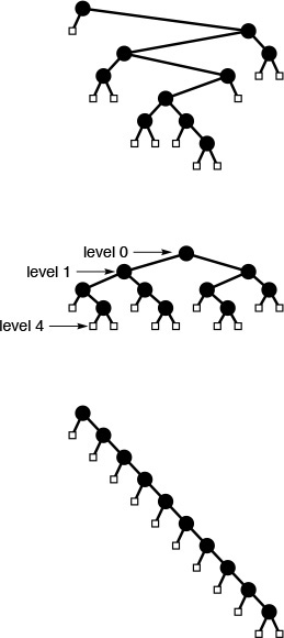
The binary tree shown at the top has height 7, internal path length 31 and external path length 51. A fully balanced binary tree (center) with 10 internal nodes has height 4, internal path length 19 and external path length 39 (no binary tree with 10 nodes has smaller values for any of these quantities). A degenerate binary tree (bottom) with 10 internal nodes has height 10, internal path length 45 and external path length 65 (no binary tree with 10 nodes has larger values for any of these quantities).
Figure 5.23 Three binary trees with 10 internal nodes
since there are N + 1 external nodes. This inequality implies the property stated: The best-case height is precisely equal to lg N rounded up to the nearest integer. ![]()
Property 5.9 The internal path length of a binary tree with N internal nodes is at least N lg(N/4) and at most N(N – 1)/2.
The worst case and the best case are achieved for the same trees referred to in the discussion of Property 5.8 and depicted in Figure 5.23. The internal path length of the worst-case tree is 0+1+2+ ... + (N – 1) = N(N – 1)/2. The best case tree has (N + 1) external nodes at height no more than ![]() lg N
lg N ![]() . Multiplying these and applying Property 5.7, we get the bound (N + 1)
. Multiplying these and applying Property 5.7, we get the bound (N + 1) ![]() lg N
lg N![]() – 2N < N lg(N/4).
– 2N < N lg(N/4). ![]()
As we shall see, binary trees appear extensively in computer applications, and performance is best when the binary trees are fully balanced (or nearly so). For example, the trees that we use to describe divide-and-conquer algorithms such as binary search and mergesort are fully balanced (see Exercise 5.74). In Chapters 9 and 13, we shall examine explicit data structures that are based on balanced trees.
These basic properties of trees provide the information that we need to develop efficient algorithms for a number of practical problems. More detailed analyses of several of the specific algorithms that we shall encounter require sophisticated mathematical analysis, although we can often get useful estimates with straightforward inductive arguments like the ones that we have used in this section. We discuss further mathematical properties of trees as needed in the chapters that follow. At this point, we are ready to move back to algorithmic matters.
Exercises
![]() 5.68 How many external nodes are there in an M-ary tree with N internal nodes? Use your answer to give the amount of memory required to represent such a tree, assuming that links and items require one word of memory each.
5.68 How many external nodes are there in an M-ary tree with N internal nodes? Use your answer to give the amount of memory required to represent such a tree, assuming that links and items require one word of memory each.
5.69 Give upper and lower bounds on the height of an M-ary tree with N internal nodes.
![]() 5.70 Give upper and lower bounds on the internal path length of an M-ary tree with N internal nodes.
5.70 Give upper and lower bounds on the internal path length of an M-ary tree with N internal nodes.
5.71 Give upper and lower bounds on the number of leaves in a binary tree with N nodes.
![]() 5.72 Show that if the levels of the external nodes in a binary tree differ by a constant, then the height is O(log N).
5.72 Show that if the levels of the external nodes in a binary tree differ by a constant, then the height is O(log N).
![]() 5.73 A Fibonacci tree of height n > 2 is a binary tree with a Fibonacci tree of height n – 1 in one subtree and a Fibonacci tree of height n – 2 in the other subtree. A Fibonacci tree of height 0 is a single external node, and a Fibonacci tree of height 1 is a single internal node with two external children (see Figure 5.14). Give the height and external path length of a Fibonacci tree of height n, as a function of N, the number of nodes in the tree.
5.73 A Fibonacci tree of height n > 2 is a binary tree with a Fibonacci tree of height n – 1 in one subtree and a Fibonacci tree of height n – 2 in the other subtree. A Fibonacci tree of height 0 is a single external node, and a Fibonacci tree of height 1 is a single internal node with two external children (see Figure 5.14). Give the height and external path length of a Fibonacci tree of height n, as a function of N, the number of nodes in the tree.
5.74 A divide-and-conquer tree of N nodes is a binary tree with a root labeled N, a divide-and-conquer tree of ![]() N/2
N/2![]() nodes in one subtree, and a divide-and-conquer tree of
nodes in one subtree, and a divide-and-conquer tree of ![]() N/2
N/2![]() nodes in the other subtree. (Figure 5.6 depicts a divide-and-conquer tree.) Draw divide-and-conquer trees with 11, 15, 16, and 23 nodes.
nodes in the other subtree. (Figure 5.6 depicts a divide-and-conquer tree.) Draw divide-and-conquer trees with 11, 15, 16, and 23 nodes.
![]() 5.75 Prove by induction that the internal path length of a divide-and-conquer tree is between N lg N and N lg N + N.
5.75 Prove by induction that the internal path length of a divide-and-conquer tree is between N lg N and N lg N + N.
5.76 A combine-and-conquer tree of N nodes is a binary tree with a root labeled N, a combine-and-conquer tree of ![]() N/2
N/2![]() nodes in one subtree, and a combine-and-conquer tree of
nodes in one subtree, and a combine-and-conquer tree of ![]() N/2
N/2![]() nodes in the other subtree (see Exercise 5.18). Draw combine-and-conquer trees with 11, 15, 16, and 23 nodes.
nodes in the other subtree (see Exercise 5.18). Draw combine-and-conquer trees with 11, 15, 16, and 23 nodes.
5.77 Prove by induction that the internal path length of a combine-and-conquer tree is between N lg N and N lg N + N.
5.78 A complete binary tree is one with all levels filled, except possibly the final one, which is filled from left to right, as illustrated in Figure 5.24. Prove that the internal path length of a complete tree with N nodes is between N lg N and N lg N + N.
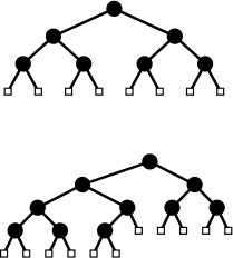
When the number of external nodes is a power of 2 (top), the external nodes in a complete binary tree are all at the same level. Otherwise (bottom), the external nodes appear on two levels, with the internal nodes to the left of the external nodes on the next-to-bottom level.
Figure 5.24 Complete binary trees with seven and 10 internal nodes
5.6 Tree Traversal
Before considering algorithms that construct binary trees and trees, we consider algorithms for the most basic tree-processing function: tree traversal: Given a pointer to a tree, we want to process every node in the tree systematically. In a linked list, we move from one node to the next by following the single link; for trees, however, we have decisions to make, because there may be multiple links to follow.
We begin by considering the process for binary trees. For linked lists, we had two basic options (see Program 5.5): process the node and then follow the link (in which case we would visit the nodes in order), or follow the link and then process the node (in which case we would visit the nodes in reverse order). For binary trees, we have two links, and we therefore have three basic orders in which we might visit the nodes:
• Preorder, where we visit the node, then visit the left and right subtrees
• Inorder, where we visit the left subtree, then visit the node, then visit the right subtree
• Postorder, where we visit the left and right subtrees, then visit the node
We can implement these methods easily with a recursive program, as shown in Program 5.14, which is a direct generalization of the linked-list–traversal program in Program 5.5. To implement traversals in the other orders, we permute the function calls in Program 5.14 in the appropriate manner. Figure 5.26 shows the order in which we visit the nodes in a sample tree for each order. Figure 5.25 shows the sequence of function calls that is executed when we invoke Program 5.14 on the sample tree in Figure 5.26.
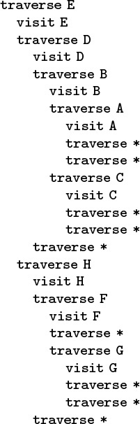
This sequence of function calls constitutes preorder traversal for the example tree in Figure 5.26.
Figure 5.25 Preorder-traversal function calls

These sequences indicate the order in which we visit nodes for preorder (left), inorder (center), and postorder (right) tree traversal.
Figure 5.26 Tree-traversal orders
We have already encountered the same basic recursive processes on which the different tree-traversal methods are based, in divide-and-conquer recursive programs (see Figures 5.8 and 5.11), and in arithmetic expressions. For example, doing preorder traversal corresponds to drawing the marks on the ruler first, then making the recursive calls (see Figure 5.11); doing inorder traversal corresponds to moving the biggest disk in the towers of Hanoi solution in between recursive calls that move all of the others; doing postorder traversal corresponds to evaluating postfix expressions, and so forth. These correspondences give us immediate insight into the mechanisms behind tree traversal. For example, we know that every other node in an inorder traversal is an external node, for the same reason that every other move in the towers of Hanoi problem involves the small disk.
It is also useful to consider nonrecursive implementations that use an explicit pushdown stack. For simplicity, we begin by considering an abstract stack that can hold items or trees, initialized with the tree to be traversed. Then, we enter into a loop, where we pop and process the top entry on the stack, continuing until the stack is empty. If the popped entity is an item, we visit it; if the popped entity is a tree, then we perform a sequence of push operations that depends on the desired ordering:
• For preorder, we push the right subtree, then the left subtree, and then the node.
• For inorder, we push the right subtree, then the node, and then the left subtree.
• For postorder, we push the node, then the right subtree, and then the left subtree.
We do not push null trees onto the stack. Figure 5.27 shows the stack contents as we use each of these three methods to traverse the sample tree in Figure 5.26. We can easily verify by induction that this method produces the same output as the recursive one for any binary tree.
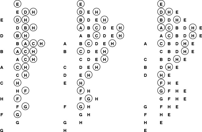
These sequences indicate the stack contents for preorder (left), inorder (center), and postorder (right) tree traversal (see Figure 5.26), for an idealized model of the computation, similar to the one that we used in Figure 5.5, where we put the item and its two subtrees on the stack, in the indicated order.
Figure 5.27 Stack contents for tree-traversal algorithms
The scheme described in the previous paragraph is a conceptual one that encompasses the three traversal methods, but the implementations that we use in practice are slightly simpler. For example, for preorder, we do not need to push nodes onto the stack (we visit the root of each tree that we pop), and we therefore can use a simple stack that contains only one type of item (tree link), as in the nonrecursive implementation in Program 5.15. The system stack that supports the recursive program contains return addresses and argument values, rather than items or nodes, but the actual sequence in which we do the computations (visit the nodes) is the same for the recursive and the stack-based methods.
A fourth natural traversal strategy is simply to visit the nodes in a tree as they appear on the page, reading down from top to bottom and from left to right. This method is called level-order traversal because all the nodes on each level appear together, in order. Figure 5.28 shows how the nodes of the tree in Figure 5.26 are visited in level order.
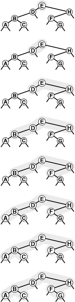
This sequence depicts the result of visiting nodes in order from top to bottom and left to right in the tree.
Figure 5.28 Level-order traversal
Remarkably, we can achieve level-order traversal by substituting a queue for the stack in Program 5.15, as shown in Program 5.16. For preorder, we use a LIFO data structure; for level order, we use a FIFO data structure. These programs merit careful study, because they represent approaches to organizing work remaining to be done that differ in an essential way. In particular, level order does not correspond to a recursive implementation relates to the recursive structure of the tree.
Preorder, postorder, and level order are well defined for forests as well. To make the definitions consistent, think of a forest as a tree with an imaginary root. Then, the preorder rule is “visit the root, then visit each of the subtrees,” the postorder rule is “visit each of the subtrees, then visit the root.” The level-order rule is the same as for binary trees. Direct implementations of these methods are straightforward generalizations of the stack-based preorder traversal programs (Programs 5.14 and 5.15) and the queue-based level-order traversal program (Program 5.16) for binary trees that we just considered. We omit consideration of implementations because we consider a more general procedure in Section 5.8.
Exercises
![]() 5.79 Give preorder, inorder, postorder, and level-order traversals of the following binary trees:
5.79 Give preorder, inorder, postorder, and level-order traversals of the following binary trees:
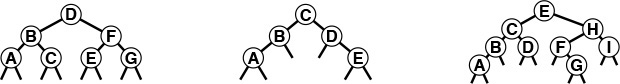
![]() 5.80 Show the contents of the queue during the level order traversal (Program 5.16) depicted in Figure 5.28, in the style of Figure 5.27.
5.80 Show the contents of the queue during the level order traversal (Program 5.16) depicted in Figure 5.28, in the style of Figure 5.27.
5.81 Show that preorder for a forest is the same as preorder for the corresponding binary tree (see Property 5.4), and that postorder for a forest is the same as inorder for the binary tree.
![]() 5.82 Give a nonrecursive implementation of inorder traversal.
5.82 Give a nonrecursive implementation of inorder traversal.
![]() 5.83 Give a nonrecursive implementation of postorder traversal.
5.83 Give a nonrecursive implementation of postorder traversal.
![]() 5.84 Write a program that takes as input the preorder and inorder traversals of a binary tree, and produces as output the level-order traversal of the tree.
5.84 Write a program that takes as input the preorder and inorder traversals of a binary tree, and produces as output the level-order traversal of the tree.
5.7 Recursive Binary-Tree Algorithms
The tree-traversal algorithms that we considered in Section 5.6 exemplify the basic fact that we are led to consider recursive algorithms for binary trees, because of these trees’ very nature as recursive structures. Many tasks admit direct recursive divide-and-conquer algorithms, which essentially generalize the traversal algorithms. We process a tree by processing the root node and (recursively) its subtrees; we can do computation before, between, or after the recursive calls (or possibly all three).
We frequently need to find the values of various structural parameters for a tree, given only a link to the tree. For example, Program 5.17 comprises recursive functions for computing the number of nodes in and the height of a given tree. The functions follow immediately from Definition 5.6. Neither of these functions depends on the order in which the recursive calls are processed: they process all the nodes in the tree and return the same answer if we, for example, exchange the recursive calls. Not all tree parameters are so easily computed: for example, a program to compute efficiently the internal path length of a binary tree is more challenging (see Exercises 5.88 through 5.90).
Another function that is useful whenever we write programs that process trees is one that prints out or draws the tree. For example, Program 5.18 is a recursive procedure that prints out a tree in the format illustrated in Figure 5.29. We can use the same basic recursive scheme to draw more elaborate representations of trees, such as those that we use in the figures in this book (see Exercise 5.85).
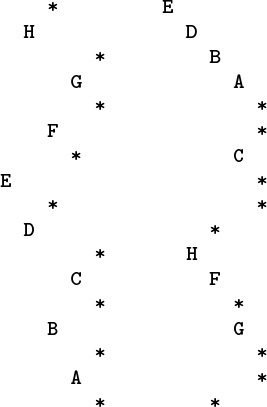
The output at the left results from using Program 5.18 on the sample tree in Figure 5.26, and exhibits the tree structure in a manner similar to the graphical representation that we have been using, rotated 90 degrees. The output at the right is from the same program with the print statement moved to the beginning; it exhibits the tree structure in a familiar outline format.
Figure 5.29 Printing a tree (inorder and preorder)
Program 5.18 is an inorder traversal—if we print the item before the recursive calls, we get a preorder traversal, which is also illustrated in Figure 5.29. This format is a familiar one that we might use, for example, for a family tree, or to list files in a tree-based file system, or to make an outline of a printed document. For example, doing a preorder traversal of the tree in Figure 5.19 gives a version of the table of contents of this book.
Our first example of a program that builds an explicit binary tree structure is associated with the find-the-maximum application that we considered in Section 5.2. Our goal is to build a tournament: a binary tree where the item in every internal node is a copy of the larger of the items in its two children. In particular, the item at the root is a copy of the largest item in the tournament. The items in the leaves (nodes with no children) constitute the data of interest, and the rest of the tree is a data structure that allows us to find the largest of the items efficiently.
Program 5.19 is a recursive program that builds a tournament from the items in an array. A modification of Program 5.6, it thus uses a divide-and-conquer recursive strategy: To build a tournament for a single item, we create (and return) a leaf containing that item. To build a tournament for N > 1 items, we use the divide-and-conquer strategy: Divide the items in half, build tournaments for each half, and create a new node with links to the two tournaments and with an item that is a copy of the larger of the items in the roots of the two tournaments.
Figure 5.30 is an example of an explicit tree structure that might be built by Program 5.19. Building a recursive data structure such as this one is perhaps preferable in some situations to finding the maximum by scanning the data, as we did in Program 5.6, because the tree structure provides us with the flexibility to perform other operations. The very operation that we use to build the tournament is an important example: Given two tournaments, we can combine them into a single tournament in constant time, by creating a new node, making its left link point to one of the tournaments and its right link point to the other, and taking the larger of the two items (at the roots of the two given tournaments) as the largest item in the combined tournament. We also can consider algorithms for adding items, removing items, and performing other operations. We shall not consider such operations in any further detail here because similar data structures with this flexibility are the topic of Chapter 9.
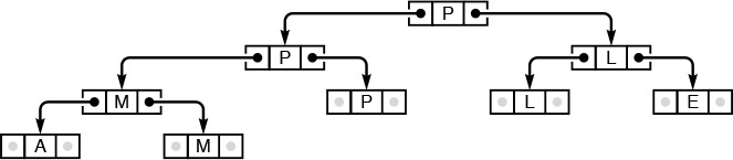
This figure depicts the explicit tree structure that is constructed by Program 5.19 from the input A M P L E. The data items are in the leaves. Each internal node has a copy of the larger of the items in its two children, so, by induction, the largest item is at the root.
Figure 5.30 Explicit tree for finding the maximum (tournament)
Indeed, tree-based implementations for several of the generalized queue ADTs that we discussed in Section 4.6 are a primary topic of discussion for much of this book. In particular, many of the algorithms in Chapters 12 through 15 are based on binary search trees, which are explicit trees that correspond to binary search, in a relationship analogous to the relationship between the explicit structure of Figure 5.30 and the recursive find-the-maximum algorithm (see Figure 5.6). The challenge in implementing and using such structures is to ensure that our algorithms remain efficient after a long sequence of insert, delete, and other operations.
Our second example of a program that builds a binary tree is a modification of our prefix-expression–evaluation program in Section 5.1 (Program 5.4) to construct a tree representing a prefix expression, instead of just evaluating it (see Figure 5.31). Program 5.20 uses the same recursive scheme as Program 5.4, but the recursive function returns a link to a tree, rather than a value. We create a new tree node for each character in the expression: Nodes corresponding to operators have links to their operands, and the leaf nodes contain the variables (or constants) that are inputs to the expression.
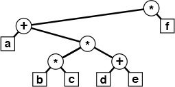
This tree is constructed by Program 5.20 for the prefix expression * + a * * b c + d e f. It is a natural way to represent the expression: Each operand is in a leaf (which we draw here as an external node), and each operator is to be applied to the expressions represented by the left and right subtrees of the node containing the operator.
Figure 5.31 Parse tree
Translation programs such as compilers often use such internal tree representations for programs, because the trees are useful for many purposes. For example, we might imagine operands corresponding to variables that take on values, and we could generate machine code to evaluate the expression represented by the tree with a postorder traversal. Or, we could use the tree to print out the expression in infix with an inorder traversal or in postfix with a postorder traversal.
We considered the few examples in this section to introduce the concept that we can build and process explicit linked tree structures with recursive programs. To do so effectively, we need to consider the performance of various algorithms, alternate representations, nonrecursive alternatives, and many other details. However, we shall defer consideration of tree-processing programs in further detail until Chapter 12, because we use trees primarily for descriptive purposes in Chapters 7 through 11. We return to explicit tree implementations in Chapter 12 because they form the basis of numerous algorithms that we consider in Chapters 12 through 15.
Exercises
![]() 5.85 Modify Program 5.18 to output a PostScript program that draws the tree, in a format like that used in Figure 5.23, but without the small boxes to represent the external nodes. Use
5.85 Modify Program 5.18 to output a PostScript program that draws the tree, in a format like that used in Figure 5.23, but without the small boxes to represent the external nodes. Use moveto and lineto to draw lines, and the user-defined operator
/node { newpath moveto currentpoint 4 0 360 arc fill} def
to draw nodes. After this definition, the call node draws a black dot at the coordinates on the stack (see Section 4.3).
![]() 5.86 Write a program that counts the leaves in a binary tree.
5.86 Write a program that counts the leaves in a binary tree.
![]() 5.87 Write a program that counts the number of nodes in a binary tree that have one external and one internal child.
5.87 Write a program that counts the number of nodes in a binary tree that have one external and one internal child.
![]() 5.88 Write a recursive program that computes the internal path length of a binary tree, using Definition 5.6.
5.88 Write a recursive program that computes the internal path length of a binary tree, using Definition 5.6.
5.89 Determine the number of function calls made by your program when it is computing the internal path length of a binary tree. Prove your answer by induction.
![]() 5.90 Write a recursive program that computes the internal path length of a binary tree in time proportional to the number of nodes in the tree.
5.90 Write a recursive program that computes the internal path length of a binary tree in time proportional to the number of nodes in the tree.
![]() 5.91 Write a recursive program that deletes all the leaves with a given key from a tournament (see Exercise 5.59).
5.91 Write a recursive program that deletes all the leaves with a given key from a tournament (see Exercise 5.59).
5.8 Graph Traversal
For our final example of a recursive program in this chapter, we consider one of the most important of all recursive programs: recursive graph traversal, or depth-first search. This method for systematically visiting all the nodes in a graph is a direct generalization of the tree-traversal methods that we considered in Section 5.6, and it serves as the basis for many basic algorithms for processing graphs (see Part 7). It is a simple recursive algorithm. Starting at any node v, we
• Visit v.
• (Recursively) visit each (unvisited) node attached to v.
If the graph is connected, we eventually reach all of the nodes. Program 5.21 is an implementation of this recursive procedure.
For example, suppose that we use the adjacency-list representation depicted in the sample graph in Figure 3.15. Figure 5.32 shows the recursive calls made during the depth-first search of this graph, and the sequence on the left in Figure 5.33 depicts the way in which we follow the edges in the graph. We follow each edge in the graph, with one of two possible outcomes: if the edge takes us to a node that we have already visited, we ignore it; if it takes us to a node that we have not yet visited, we follow it there via a recursive call. The set of all edges that we follow in this way forms a spanning tree for the graph.
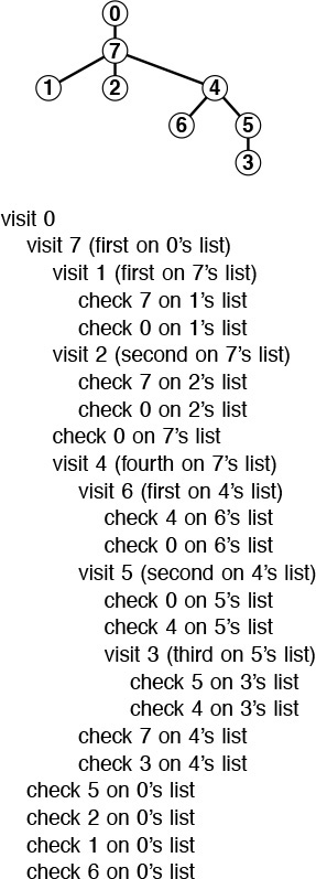
This sequence of function calls constitutes depth-first search for the example graph in Figure 3.15. The tree that depicts the recursive-call structure (top) is called the depth-first–search tree.
Figure 5.32 Depth-first–search function calls
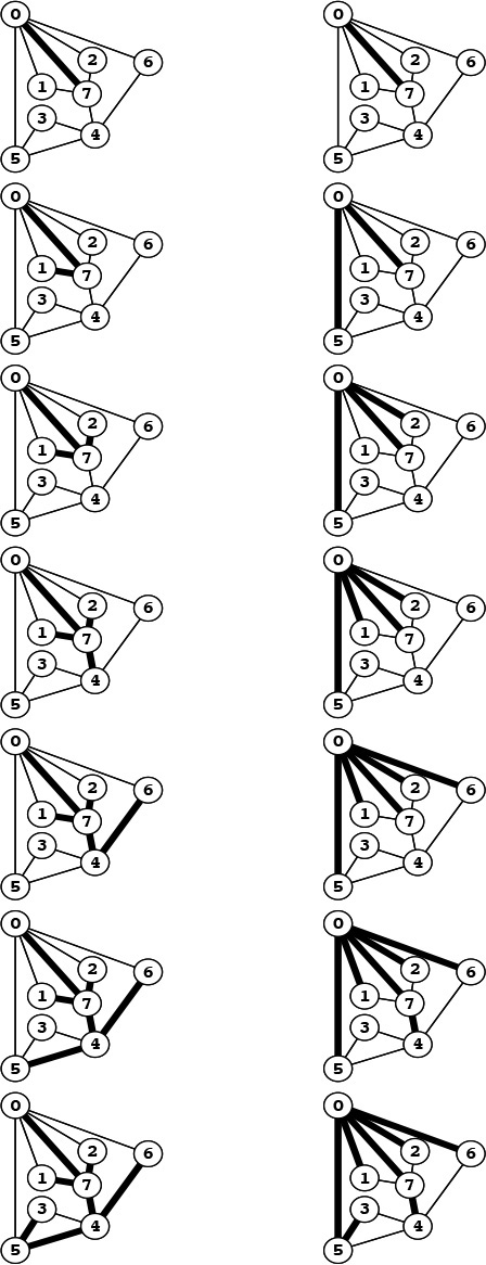
Depth-first search (left) moves from node to node, backing up to the previous node to try the next possibility whenever it has tried every possibility at a given node. Breadth-first search (right) exhausts all the possibilities at one node before moving to the next.
Figure 5.33 Depth-first search and breadth-first search
The difference between depth-first search and general tree traversal (see Program 5.14) is that we need to guard explicitly against visiting nodes that we have already visited. In a tree, we never encounter any such nodes. Indeed, if the graph is a tree, recursive depth-first search starting at the root is equivalent to preorder traversal.
Property 5.10 Depth-first search requires time proportional to V + E in a graph with V vertices and E edges, using the adjacency lists representation.
In the adjacency lists representation, there is one list node corresponding to each edge in the graph, and one list head pointer corresponding to each vertex in the graph. Depth-first search touches all of them, at most once. ![]()
Because it also takes time proportional to V + E to build the adjacency lists representation from an input sequence of edges (see Program 3.19), depth-first search gives us a linear-time solution to the connectivity problem of Chapter 1. For huge graphs, however, the union–find solutions might still be preferable, because representing the whole graph takes space proportional to E, while the union–find solutions take space only proportional to V.
As we did with tree traversal, we can define a graph-traversal method that uses an explicit stack, as depicted in Figure 5.34. We can think of an abstract stack that holds dual entries: a node and a pointer into that node’s adjacency list. With the stack initialized to the start node and a pointer initialized to the first node on that node’s adjacency list, the depth-first search algorithm is equivalent to entering into a loop, where we visit the node at the top of the stack (if it has not already been visited); save the node referenced by the current adjacency-list pointer; update the adjacency list reference to the next node (popping the entry if at the end of the adjacency list); and push a stack entry for the saved node, referencing the first node on its adjacency list.
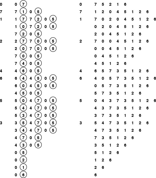
We can think of the pushdown stack supporting depth-first search as containing a node and a reference to that node’s adjacency list (indicated by a circled node) (left). Thus, we begin with node 0 on the stack, with reference to the first node on its list, node 7. Each line indicates the result of popping the stack, pushing a reference to the next node on the list for nodes that have been visited, and pushing an entry on the stack for nodes that have not been visited. Alternatively, we can think of the process as simply pushing all nodes adjacent to any unvisited node onto the stack (right).
Figure 5.34 Depth-first–search stack dynamics
Alternatively, as we did for tree traversal, we can consider the stack to contain links to nodes only. With the stack initialized to the start node, we enter into a loop where we visit the node at the top of the stack (if it has not already been visited), then push all the nodes adjacent to it onto the stack. Figure 5.34 illustrates that both of these methods are equivalent to depth-first search for our example graph, and the equivalence indeed holds in general.
The visit-the-top-node-and-push-all-its-neighbors algorithm is a simple formulation of depth-first search, but it is clear from Figure 5.34 that it suffers the disadvantage of possibly leaving multiple copies of each node on the stack. It does so even if we test whether each node that is about to go on the stack has been visited and refrain from putting the node in the stack if it has been. To avoid this problem, we can use a stack implementation that disallows duplicates by using a forget-the-old-item policy, because the copy nearest the top of the stack is always the first one visited, so the others are simply popped.
The stack dynamics for depth-first search that are illustrated in Figure 5.34 depend on the nodes on each adjacency list ending up on the stack in the same order that they appear in the list. To get this ordering for a given adjacency list when pushing one node at a time, we would have to push the last node first, then the next-to-last node, and so forth. Moreover, to limit the stack size to the number of vertices while at the same time visiting the nodes in the same order as in depth-first search, we need to use a stack discipline with a forget-the-old-item policy. If visiting the nodes in the same order as depth-first search is not important to us, we can avoid both of these complications and directly formulate a nonrecursive stack-based graph-traversal method: With the stack initialized to the start node, we enter into a loop where we visit the node at the top of the stack, then proceed through its adjacency list, pushing each node onto the stack (if the node has not been visited already), using a stack implementation that disallows duplicates with an ignore-the-new-item policy. This algorithm visits all the nodes in the graph in a manner similar to depth-first-search, but it is not recursive.
The algorithm in the previous paragraph is noteworthy because we could use any generalized queue ADT, and still visit each of the nodes in the graph (and generate a spanning tree). For example, if we use a queue instead of a stack, then we have breadth-first search, which is analogous to level-order traversal in a tree. Program 5.22 is an implementation of this method (assuming that we use a queue implementation like Program 4.12); an example of the algorithm in operation is depicted in Figure 5.35. In Part 6, we shall examine numerous graph algorithms based on more sophisticated generalized queue ADTs.
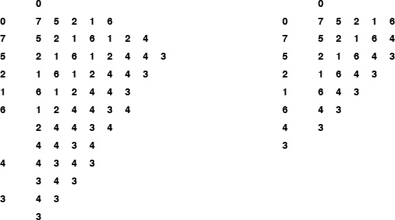
We start with 0 on the queue, then get 0, visit it, and put the nodes on its adjacency list 7 5 2 1 6, in that order onto the queue. Then we get 7, visit it, and put the nodes on its adjacency list, and so forth. With duplicates disallowed with an ignore-the-new-item policy (right), we get the same result without any extraneous queue entries.
Figure 5.35 Breadth-first–search queue dynamics
Breadth-first search and depth-first search both visit all the nodes in a graph, but their manner of doing so is dramatically different, as illustrated in Figure 5.36. Breadth-first search amounts to an army of searchers fanning out to cover the territory; depth-first search corresponds to a single searcher probing unknown territory as deeply as possible, retreating only when hitting dead ends. These are basic problem-solving paradigms of significance in many areas of computer science beyond graph searching.
This diagram shows depth-first search (center) and breadth-first search (bottom), halfway through searching in a large graph (top). Depth-first search meanders from one node to the next, so most nodes are connected to just two others. By contrast, breadth-first search sweeps through the graph, visiting all the nodes connected to a given node before moving on, so several nodes are connected to many others.
Figure 5.36 Graph-traversal trees
Exercises
5.92 Show how recursive depth-first search visits the nodes in the graph built for the edge sequence 0-2, 1-4, 2-5, 3-6, 0-4, 6-0, and 1-3 (see Exercise 3.70), by giving diagrams corresponding to Figures 5.33 (left) and 5.34 (right).
5.93 Show how stack-based depth-first search visits the nodes in the graph built for the edge sequence 0-2, 1-4, 2-5, 3-6, 0-4, 6-0, and 1-3, by giving diagrams corresponding to Figures 5.33 (left) and 5.34 (right).
5.94 Show how (queue-based) breadth-first search visits the nodes in the graph built for the edge sequence 0-2, 1-4, 2-5, 3-6, 0-4, 6-0, and 1-3, by giving diagrams corresponding to Figures 5.33 (right) and 5.35 (left).
![]() 5.95 Why is the running time in Property 5.10 quoted as V + E and not simply E?
5.95 Why is the running time in Property 5.10 quoted as V + E and not simply E?
5.96 Show how stack-based depth-first search visits the nodes in the example graph in the text (Figure 3.15) when using a forget-the-old-item policy, by giving diagrams corresponding to Figures 5.33 (left) and 5.35 (right).
5.97 Show how stack-based depth-first search visits the nodes in the example graph in the text (Figure 3.15) when using an ignore-the-new-item policy, by giving diagrams corresponding to Figures 5.33 (left) and 5.35 (right).
![]() 5.98 Implement a stack-based depth-first search for graphs that are represented with adjacency lists.
5.98 Implement a stack-based depth-first search for graphs that are represented with adjacency lists.
![]() 5.99 Implement a recursive depth-first search for graphs that are represented with adjacency lists.
5.99 Implement a recursive depth-first search for graphs that are represented with adjacency lists.
5.9 Perspective
Recursion lies at the heart of early theoretical studies into the nature of computation. Recursive functions and programs play a central role in mathematical studies that attempt to separate problems that can be solved by a computer from problems that cannot be.
It is certainly impossible to do justice to topics as far-reaching as trees and recursion in so brief a discussion. Many of the best examples of recursive programs will be our focus throughout the book—divide-and-conquer algorithms and recursive data structures that have been applied successfully to solve a wide variety of problems. For many applications, there is no reason to go beyond a simple, direct recursive implementation; for others, we will consider the derivation of alternate nonrecursive and bottom-up implementations.
In this book, our interest lies in the practical aspects of recursive programs and data structures. Our goal is to exploit recursion to produce elegant and efficient implementations. To meet that goal, we need to have particular respect for the dangers of simple programs that lead to an exponential number of function calls or impossibly deep nesting. Despite this pitfall, recursive programs and data structures are attractive because they often provide us with inductive arguments that can convince us that our programs are correct and efficient.
We use trees throughout the book, both to help us understand the dynamic properties of programs, and as dynamic data structures. Chapters 12 through 15 in particular are largely devoted to the manipulation of explicit tree structures. The properties described in this chapter provide us with the basic information that we need if we are to use explicit tree structures effectively.
Despite its central role in algorithm design, recursion is not a panacea. As we discovered in our study of tree- and graph-traversal algorithms, stack-based (inherently recursive) algorithms are not the only option when we have multiple computational tasks to manage. An effective algorithm-design technique for many problems is the use of generalized queue implementations other than stacks to give us the freedom to choose the next task according to some more subjective criteria than simply choosing the most recent. Data structures and algorithms that efficiently support such operations are a prime topic of Chapter 9, and we shall encounter many examples of their application when we consider graph algorithms in Part 7.