Chapter Two. Principles of Algorithm Analysis
Analysis is the key to being able to understand algorithms sufficiently well that we can apply them effectively to practical problems. Although we cannot do extensive experimentation and deep mathematical analysis on each and every program that we run, we can work within a basic framework involving both empirical testing and approximate analysis that can help us to know the important facts about the performance characteristics of our algorithms, so that we may compare those algorithms and can apply them to practical problems.
The very idea of describing the performance of a complex algorithm accurately with a mathematical analysis seems a daunting prospect at first, and we do often call on the research literature for results based on detailed mathematical study. Although it is not our purpose in this book to cover methods of analysis or even to summarize these results, it is important for us to be aware at the outset that we are on firm scientific ground when we want to compare different methods. Moreover, a great deal of detailed information is available about many of our most important algorithms through careful application of relatively few elementary techniques. We do highlight basic analytic results and methods of analysis throughout the book, particularly when such understanding helps us to understand the inner workings of fundamental algorithms. Our primary goal in this chapter is to provide the context and the tools that we need to work intelligently with the algorithms themselves.
The example in Chapter 1 provides a context that illustrates many of the basic concepts of algorithm analysis, so we frequently refer back to the performance of union-find algorithms to make particular points concrete. We also consider a detailed pair of new examples, in Section 2.6.
Analysis plays a role at every point in the process of designing and implementing algorithms. At first, as we saw, we can save factors of thousands or millions in the running time with appropriate algorithm design choices. As we consider more efficient algorithms, we find it more of a challenge to choose among them, so we need to study their properties in more detail. In pursuit of the best (in some precise technical sense) algorithm, we find both algorithms that are useful in practice and theoretical questions that are challenging to resolve.
Complete coverage of methods for the analysis of algorithms is the subject of a book in itself (see reference section), but it is worthwhile for us to consider the basics here, so that we can
• Illustrate the process.
• Describe in one place the mathematical conventions that we use.
• Provide a basis for discussion of higher-level issues.
• Develop an appreciation for scientific underpinnings of the conclusions that we draw when comparing algorithms.
Most important, algorithms and their analyses are often intertwined. In this book, we do not delve into deep and difficult mathematical derivations, but we do use sufficient mathematics to be able to understand what our algorithms are and how we can use them effectively.
2.1 Implementation and Empirical Analysis
We design and develop algorithms by layering abstract operations that help us to understand the essential nature of the computational problems that we want to solve. In theoretical studies, this process, although valuable, can take us far afield from the real-world problems that we need to consider. Thus, in this book, we keep our feet on the ground by expressing all the algorithms that we consider in an actual programming language: C. This approach sometimes leaves us with a blurred distinction between an algorithm and its implementation, but that is small price to pay for the ability to work with and to learn from a concrete implementation.
Indeed, carefully constructed programs in an actual programming language provide an effective means of expressing our algorithms. In this book, we consider a large number of important and efficient algorithms that we describe in implementations that are both concise and precise in C. English-language descriptions or abstract high-level representations of algorithms are all too often vague or incomplete; actual implementations force us to discover economical representations to avoid being inundated in detail.
We express our algorithms in C, but this book is about algorithms, rather than about C programming. Certainly, we consider C implementations for many important tasks, and, when there is a particularly convenient or efficient way to do a task in C, we will take advantage of it. But the vast majority of the implementation decisions that we make are worth considering in any modern programming environment. Translating the programs in Chapter 1, and most of the other programs in this book, to another modern programming language is a straightforward task. On occasion, we also note when some other language provides a particularly effective mechanism suited to the task at hand. Our goal is to use C as a vehicle for expressing the algorithms that we consider, rather than to dwell on implementation issues specific to C.
If an algorithm is to be implemented as part of a large system, we use abstract data types or a similar mechanism to make it possible to change algorithms or implementations after we determine what part of the system deserves the most attention. From the start, however, we need to have an understanding of each algorithm’s performance characteristics, because design requirements of the system may have a major influence on algorithm performance. Such initial design decisions must be made with care, because it often does turn out, in the end, that the performance of the whole system depends on the performance of some basic algorithm, such as those discussed in this book.
Implementations of the algorithms in this book have been put to effective use in a wide variety of large programs, operating systems, and applications systems. Our intention is to describe the algorithms and to encourage a focus on their dynamic properties through experimentation with the implementations given. For some applications, the implementations may be quite useful exactly as given; for other applications, however, more work may be required. For example, using a more defensive programming style than the one that we use in this book is justified when we are building real systems. Error conditions must be checked and reported, and programs must be implemented such that they can be changed easily, read and understood quickly by other programmers, interface well with other parts of the system, and be amenable to being moved to other environments.
Notwithstanding all these comments, we take the position when analyzing each algorithm that performance is of critical importance, to focus our attention on the algorithm’s essential performance characteristics. We assume that we are always interested in knowing about algorithms with substantially better performance, particularly if they are simpler.
To use an algorithm effectively, whether our goal is to solve a huge problem that could not otherwise be solved, or whether our goal is to provide an efficient implementation of a critical part of a system, we need to have an understanding of its performance characteristics. Developing such an understanding is the goal of algorithmic analysis.
One of the first steps that we take to understand the performance of algorithms is to do empirical analysis. Given two algorithms to solve the same problem, there is no mystery in the method: We run them both to see which one takes longer! This concept might seem too obvious to mention, but it is an all-too-common omission in the comparative study of algorithms. The fact that one algorithm is 10 times faster than another is unlikely to escape the notice of someone who waits 3 seconds for one to finish and 30 seconds for the other to finish, but it is easy to overlook as a small constant overhead factor in a mathematical analysis. When we monitor the performance of careful implementations on typical input, we get performance results that not only give us a direct indicator of efficiency, but also provide us with the information that we need to compare algorithms and to validate any mathematical analyses that may apply (see, for example, Table 1.1). When empirical studies start to consume a significant amount of time, mathematical analysis is called for. Waiting an hour or a day for a program to finish is hardly a productive way to find out that it is slow, particularly when a straightforward analysis can give us the same information.
For many applications, our only chance to be able to solve huge problem instances is to use an efficient algorithm. This table indicates the minimum amount of time required to solve problems of size 1 million and 1 billion, using linear, N log N, and quadratic algorithms, on computers capable of executing 1 million, 1 billion, and 1 trillion instructions per second. A fast algorithm enables us to solve a problem on a slow machine, but a fast machine is no help when we are using a slow algorithm.
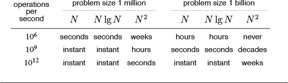
Table 2.1 Time to solve huge problems
The first challenge that we face in empirical analysis is to develop a correct and complete implementation. For some complex algorithms, this challenge may present a significant obstacle. Accordingly, we typically want to have, through analysis or through experience with similar programs, some indication of how efficient a program might be before we invest too much effort in getting it to work.
The second challenge that we face in empirical analysis is to determine the nature of the input data and other factors that have direct influence on the experiments to be performed. Typically, we have three basic choices: use actual data, random data, or perverse data. Actual data enable us truly to measure the cost of the program in use; random data assure us that our experiments test the algorithm, not the data; and perverse data assure us that our programs can handle any input presented them. For example, when we test sorting algorithms, we run them on data such as the words in Moby Dick, on randomly generated integers, and on files of numbers that are all the same value. This problem of determining which input data to use to compare algorithms also arises when we analyze the algorithms.
It is easy to make mistakes when we compare implementations, particularly if differing machines, compilers, or systems are involved, or if huge programs with ill-specified inputs are being compared. The principal danger in comparing programs empirically is that one implementation may be coded more carefully than the other. The inventor of a proposed new algorithm is likely to pay careful attention to every aspect of its implementation, and not to expend so much effort on the details of implementing a classical competing algorithm. To be confident of the accuracy of an empirical study comparing algorithms, we must be sure to give the same attention to each implementation.
One approach that we often use in this book, as we saw in Chapter 1, is to derive algorithms by making relatively minor modifications to other algorithms for the same problem, so comparative studies really are valid. More generally, we strive to identify essential abstract operations, and start by comparing algorithms on the basis of their use of such operations. For example, the comparative empirical results that we examined in Table 1.1 are likely to be robust across programming languages and environments, as they involve programs that are similar and that make use of the same set of basic operations. For a particular programming environment, we can easily relate these numbers to actual running times. Most often, we simply want to know which of two programs is likely to be faster, or to what extent a certain change will improve the time or space requirements of a certain program.
Choosing among algorithms to solve a given problem is tricky business. Perhaps the most common mistake made in selecting an algorithm is to ignore performance characteristics. Faster algorithms are often more complicated than brute-force solutions, and implementors are often willing to accept a slower algorithm to avoid having to deal with added complexity. As we saw with union-find algorithms, however, we can sometimes reap huge savings with just a few lines of code. Users of a surprising number of computer systems lose substantial time waiting for simple quadratic algorithms to finish when N log N algorithms are available that are only slightly more complicated and could run in a fraction of the time. When we are dealing with huge problem sizes, we have no choice but to seek a better algorithm, as we shall see.
Perhaps the second most common mistake made in selecting an algorithm is to pay too much attention to performance characteristics. Improving the running time of a program by a factor of 10 is inconsequential if the program takes only a few microseconds. Even if a program takes a few minutes, it may not be worth the time and effort required to make it run 10 times faster, particularly if we expect to use the program only a few times. The total time required to implement and debug an improved algorithm might be substantially more than the time required simply to run a slightly slower one—we may as well let the computer do the work. Worse, we may spend a considerable amount of time and effort implementing ideas that should improve a program but actually do not do so.
We cannot run empirical tests for a program that is not yet written, but we can analyze properties of the program and estimate the potential effectiveness of a proposed improvement. Not all putative improvements actually result in performance gains, and we need to understand the extent of the savings realized at each step. Moreover, we can include parameters in our implementations, and can use analysis to help us set the parameters. Most important, by understanding the fundamental properties of our programs and the basic nature of the programs’ resource usage, we hold the potentials to evaluate their effectiveness on computers not yet built and to compare them against new algorithms not yet designed. In Section 2.2, we outline our methodology for developing a basic understanding of algorithm performance.
Exercises
2.1 Translate the programs in Chapter 1 to another programming language, and answer Exercise 1.22 for your implementations.
2.2 How long does it take to count to 1 billion (ignoring overflow)? Determine the amount of time it takes the program
int i, j, k, count = 0;
for (i = 0; i < N; i++)
for (j = 0; j < N; j++)
for (k = 0; k < N; k++)
count++;
to complete in your programming environment, for N = 10, 100, and 1000. If your compiler has optimization features that are supposed to make programs more efficient, check whether or not they do so for this program.
2.2 Analysis of Algorithms
In this section, we outline the framework within which mathematical analysis can play a role in the process of comparing the performance of algorithms, to lay a foundation for us to be able to consider basic analytic results as they apply to the fundamental algorithms that we consider throughout the book. We shall consider the basic mathematical tools that are used in the analysis of algorithms, both to allow us to study classical analyses of fundamental algorithms and to make use of results from the research literature that help us understand the performance characteristics of our algorithms.
The following are among the reasons that we perform mathematical analysis of algorithms:
• To compare different algorithms for the same task
• To predict performance in a new environment
• To set values of algorithm parameters
We shall see many examples of each of these reasons throughout the book. Empirical analysis might suffice for some of these tasks, but mathematical analysis can be more informative (and less expensive!), as we shall see.
The analysis of algorithms can be challenging indeed. Some of the algorithms in this book are well understood, to the point that accurate mathematical formulas are known that can be used to predict running time in practical situations. People develop such formulas by carefully studying the program, to find the running time in terms of fundamental mathematical quantities, and then doing a mathematical analysis of the quantities involved. On the other hand, the performance properties of other algorithms in this book are not fully understood—perhaps their analysis leads to unsolved mathematical questions, or perhaps known implementations are too complex for a detailed analysis to be reasonable, or (most likely) perhaps the types of input that they encounter cannot be characterized accurately.
Several important factors in a precise analysis are usually outside a given programmer’s domain of influence. First, C programs are translated into machine code for a given computer, and it can be a challenging task to figure out exactly how long even one C statement might take to execute (especially in an environment where resources are being shared, so even the same program can have varying performance characteristics at two different times). Second, many programs are extremely sensitive to their input data, and performance might fluctuate wildly depending on the input. Third, many programs of interest are not well understood, and specific mathematical results may not be available. Finally, two programs might not be comparable at all: one may run much more efficiently on one particular kind of input, the other runs efficiently under other circumstances.
All these factors notwithstanding, it is often possible to predict precisely how long a particular program will take, or to know that one program will do better than another in particular situations. Moreover, we can often acquire such knowledge by using one of a relatively small set of mathematical tools. It is the task of the algorithm analyst to discover as much information as possible about the performance of algorithms; it is the task of the programmer to apply such information in selecting algorithms for particular applications. In this and the next several sections, we concentrate on the idealized world of the analyst. To make effective use of our best algorithms, we need to be able to step into this world, on occasion.
The first step in the analysis of an algorithm is to identify the abstract operations on which the algorithm is based, to separate the analysis from the implementation. Thus, for example, we separate the study of how many times one of our union-find implementations executes the code fragment i = a[i] from the analysis of how many nanoseconds might be required to execute that particular code fragment on our computer. We need both these elements to determine the actual running time of the program on a particular computer. The former is determined by properties of the algorithm; the latter by properties of the computer. This separation often allows us to compare algorithms in a way that is independent of particular implementations or of particular computers.
Although the number of abstract operations involved can be large, in principle, the performance of an algorithm typically depends on only a few quantities, and typically the most important quantities to analyze are easy to identify. One way to identify them is to use a profiling mechanism (a mechanism available in many C implementations that gives instruction-frequency counts) to determine the most frequently executed parts of the program for some sample runs. Or, like the union-find algorithms of Section 1.3, our implementation might be built on a few abstract operations. In either case, the analysis amounts to determining the frequency of execution of a few fundamental operations. Our modus operandi will be to look for rough estimates of these quantities, secure in the knowledge that we can undertake a fuller analysis for important programs when necessary. Moreover, as we shall see, we can often use approximate analytic results in conjunction with empirical studies to predict performance accurately.
We also have to study the data, and to model the input that might be presented to the algorithm. Most often, we consider one of two approaches to the analysis: we either assume that the input is random, and study the average-case performance of the program, or we look for perverse input, and study the worst-case performance of the program. The process of characterizing random inputs is difficult for many algorithms, but for many other algorithms it is straightforward and leads to analytic results that provide useful information. The average case might be a mathematical fiction that is not representative of the data on which the program is being used, and the worst case might be a bizarre construction that would never occur in practice, but these analyses give useful information on performance in most cases. For example, we can test analytic results against empirical results (see Section 2.1). If they match, we have increased confidence in both; if they do not match, we can learn about the algorithm and the model by studying the discrepancies.
In the next three sections, we briefly survey the mathematical tools that we shall be using throughout the book. This material is outside our primary narrative thrust, and readers with a strong background in mathematics or readers who are not planning to check our mathematical statements on the performance of algorithms in detail may wish to skip to Section 2.6 and to refer back to this material when warranted later in the book. The mathematical underpinnings that we consider, however, are generally not difficult to comprehend, and they are too close to core issues of algorithm design to be ignored by anyone wishing to use a computer effectively.
First, in Section 2.3, we consider the mathematical functions that we commonly need to describe the performance characteristics of algorithms. Next, in Section 2.4, we consider the O-notation, and the notion of is proportional to, which allow us to suppress detail in our mathematical analyses. Then, in Section 2.5, we consider recurrence relations, the basic analytic tool that we use to capture the performance characteristics of an algorithm in a mathematical equation. Following this survey, we consider examples where we use the basic tools to analyze specific algorithms, in Section 2.6.
Exercises
![]() 2.3 Develop an expression of the form c0 + c1N + c2N2 + c3N3 that accurately describes the running time of your program from Exercise 2.2. Compare the times predicted by this expression with actual times, for N = 10, 100, and 1000.
2.3 Develop an expression of the form c0 + c1N + c2N2 + c3N3 that accurately describes the running time of your program from Exercise 2.2. Compare the times predicted by this expression with actual times, for N = 10, 100, and 1000.
![]() 2.4 Develop an expression that accurately describes the running time of Program 1.1 in terms of M and N.
2.4 Develop an expression that accurately describes the running time of Program 1.1 in terms of M and N.
2.3 Growth of Functions
Most algorithms have a primary parameter N that affects the running time most significantly. The parameter N might be the degree of a polynomial, the size of a file to be sorted or searched, the number of characters in a text string, or some other abstract measure of the size of the problem being considered: it is most often directly proportional to the size of the data set being processed. When there is more than one such parameter (for example, M and N in the union-find algorithms that we discussed in Section 1.3), we often reduce the analysis to just one parameter by expressing one of the parameters as a function of the other or by considering one parameter at a time (holding the other constant), so we can restrict ourselves to considering a single parameter N without loss of generality. Our goal is to express the resource requirements of our programs (most often running time) in terms of N, using mathematical formulas that are as simple as possible and that are accurate for large values of the parameters. The algorithms in this book typically have running times proportional to one of the following functions:
1 Most instructions of most programs are executed once or at most only a few times. If all the instructions of a program have this property, we say that the program’s running time is constant.
log N When the running time of a program is logarithmic, the program gets slightly slower as N grows. This running time commonly occurs in programs that solve a big problem by transformation into a series of smaller problems, cutting the problem size by some constant fraction at each step. For our range of interest, we can consider the running time to be less than a large constant. The base of the logarithm changes the constant, but not by much: When N is 1 thousand, log N is 3 if the base is 10, or is about 10 if the base is 2; when N is 1 million, log N is only double these values. Whenever N doubles, log N increases by a constant, but log N does not double until N increases to N2.
N When the running time of a program is linear, it is generally the case that a small amount of processing is done on each input element. When N is 1 million, then so is the running time. Whenever N doubles, then so does the running time. This situation is optimal for an algorithm that must process N inputs (or produce N outputs).
N log N The N log N running time arises when algorithms solve a problem by breaking it up into smaller subproblems, solving them independently, and then combining the solutions. For lack of a better adjective (linearithmic?), we simply say that the running time of such an algorithm is N log N. When N is 1 million, N log N is perhaps 20 million. When N doubles, the running time more (but not much more) than doubles.
N2 When the running time of an algorithm is quadratic, that algorithm is practical for use on only relatively small problems. Quadratic running times typically arise in algorithms that process all pairs of data items (perhaps in a double nested loop). When N is 1 thousand, the running time is 1 million. Whenever N doubles, the running time increases fourfold.
N3 Similarly, an algorithm that processes triples of data items (perhaps in a triple-nested loop) has a cubic running time and is practical for use on only small problems. When N is 100, the running time is 1 million. Whenever N doubles, the running time increases eightfold.
2N Few algorithms with exponential running time are likely to be appropriate for practical use, even though such algorithms arise naturally as brute-force solutions to problems. When N is 20, the running time is 1 million. Whenever N doubles, the running time squares!
The running time of a particular program is likely to be some constant multiplied by one of these terms (the leading term) plus some smaller terms. The values of the constant coefficient and the terms included depend on the results of the analysis and on implementation details. Roughly, the coefficient of the leading term has to do with the number of instructions in the inner loop: At any level of algorithm design, it is prudent to limit the number of such instructions. For large N, the effect of the leading term dominates; for small N or for carefully engineered algorithms, more terms may contribute and comparisons of algorithms are more difficult. In most cases, we will refer to the running time of programs simply as “linear,” “N log N,” “cubic,” and so forth. We consider the justification for doing so in detail in Section 2.4.
Eventually, to reduce the total running time of a program, we focus on minimizing the number of instructions in the inner loop. Each instruction comes under scrutiny: Is it really necessary? Is there a more efficient way to accomplish the same task? Some programmers believe that the automatic tools provided by modern compilers can produce the best machine code; others believe that the best route is to hand-code inner loops into machine or assembly language. We normally stop short of considering optimization at this level, although we do occasionally take note of how many machine instructions are required for certain operations, to help us understand why one algorithm might be faster than another in practice.
For small problems, it makes scant difference which method we use—a fast modern computer will complete the job in an instant. But as problem size increases, the numbers we deal with can become huge, as indicated in Table 2.2. As the number of instructions to be executed by a slow algorithm becomes truly huge, the time required to execute those instructions becomes infeasible, even for the fastest computers. Figure 2.1 gives conversion factors from large numbers of seconds to days, months, years, and so forth; Table 2.1 gives examples showing how fast algorithms are more likely than fast computers to be able to help us solve problems without facing outrageous running times.
This table indicates the relative size of some of the functions that we encounter in the analysis of algorithms. The quadratic function clearly dominates, particularly for large N, and differences among smaller functions may not be as we might expect for small N. For example, N3/2 should be greater than N lg2 N for huge values of N, but N lg2 N is greater for the smaller values of N that might occur in practice. A precise characterization of the running time of an algorithm might involve linear combinations of these functions. We can easily separate fast algorithms from slow ones because of vast differences between, for example, lg N and N or N and N2, but distinguishing among fast algorithms involves careful study.
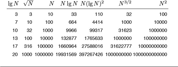
Table 2.2 Values of commonly encountered functions
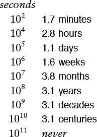
The vast difference between numbers such as 104 and 108 is more obvious when we consider them to measure time in seconds and convert to familiar units of time. We might let a program run for 2.8 hours, but we would be unlikely to contemplate running a program that would take at least 3.1 years to complete. Because 210 is approximately 103, this table is useful for powers of 2 as well. For example, 232 seconds is about 124 years.
Figure 2.1 Seconds conversions
A few other functions do arise. For example, an algorithm with N2 inputs that has a running time proportional to N3 is best thought of as an N3/2 algorithm. Also, some algorithms have two stages of subproblem decomposition, which lead to running times proportional to N log2 N. It is evident from Table 2.2 that both of these functions are much closer to N log N than to N2.
The logarithm function plays a special role in the design and analysis of algorithms, so it is worthwhile for us to consider it in detail. Because we often deal with analytic results only to within a constant factor, we use the notation “log N” without specifying the base. Changing the base from one constant to another changes the value of the logarithm by only a constant factor, but specific bases normally suggest themselves in particular contexts. In mathematics, the natural logarithm (base e = 2.71828 ...) is so important that a special abbreviation is commonly used: loge N ≡ ln N. In computer science, the binary logarithm (base 2) is so important that the abbreviation log2 N ≡ lg N is commonly used.
Occasionally, we iterate the logarithm: We apply it successively to a huge number. For example, lg lg 2256 = lg 256 = 8. As illustrated by this example, we generally regard log log N as a constant, for practical purposes, because it is so small, even when N is huge.
The smallest integer larger than lg N is the number of bits required to represent N in binary, in the same way that the smallest integer larger than log10 N is the number of digits required to represent N in decimal. The C statement
for (lgN = 0; N > 0; lgN++, N /= 2) ;
is a simple way to compute the smallest integer larger than lg N. A similar method for computing this function is
for (lgN = 0, t = 1; t < N; lgN++, t += t) ;
This version emphasizes that 2n ≤ N < 2n+1 when n is the smallest integer larger than lg N.
We also frequently encounter a number of special functions and mathematical notations from classical analysis that are useful in providing concise descriptions of properties of programs. Table 2.3 summarizes the most familiar of these functions; we briefly discuss them and some of their most important properties in the following paragraphs.
This table summarizes the mathematical notation that we use for functions and constants that arise in formulas describing the performance of algorithms. The formulas for the approximate values extend to provide much more accuracy, if desired (see reference section).
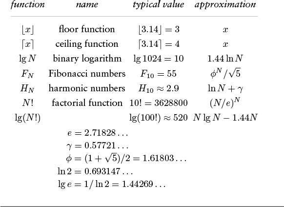
Table 2.3 Special functions and constants
Our algorithms and analyses most often deal with discrete units, so we often have need for the following special functions to convert real numbers to integers:
![]() x
x![]() : largest integer less than or equal to x
: largest integer less than or equal to x
![]() x
x![]() : smallest integer greater than or equal to x.
: smallest integer greater than or equal to x.
For example, ![]() π
π![]() and
and ![]() e
e![]() are both equal to 3, and
are both equal to 3, and ![]() lg(N + 1)
lg(N + 1)![]() is the number of bits in the binary representation of N. Another important use of these functions arises when we want to divide a set of N objects in half. We cannot do so exactly if N is odd, so, to be precise, we divide into one subset with
is the number of bits in the binary representation of N. Another important use of these functions arises when we want to divide a set of N objects in half. We cannot do so exactly if N is odd, so, to be precise, we divide into one subset with ![]() N/2
N/2![]() objects and another subset with
objects and another subset with ![]() N/2
N/2![]() objects. If N is even, the two subsets are equal in size (
objects. If N is even, the two subsets are equal in size (![]() N/2
N/2![]() =
= ![]() N/2
N/2![]() ); if N is odd, they differ in size by 1 (
); if N is odd, they differ in size by 1 (![]() N/2
N/2![]() + 1 =
+ 1 = ![]() N/2
N/2![]() ). In C, we can compute these functions directly when we are operating on integers (for example, if N ≥ 0, then
). In C, we can compute these functions directly when we are operating on integers (for example, if N ≥ 0, then N/2 is ![]() N/2
N/2![]() and
and N – (N/2) is ![]() N/2
N/2![]() ), and we can use
), and we can use floor and ceil from math.h to compute them when we are operating on floating point numbers.
A discretized version of the natural logarithm function called the harmonic numbers often arises in the analysis of algorithms. The Nth harmonic number is defined by the equation
The natural logarithm ln N is the area under the curve 1/x between 1 and N; the harmonic number HN is the area under the step function that we define by evaluating 1/x at the integers between 1 and N. This relationship is illustrated in Figure 2.2. The formula
HN ≈ ln N + γ + 1/(12N),
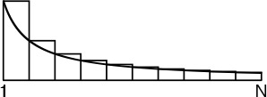
The harmonic numbers are an approximation to the area under the curve y = 1/x. The constant γ accounts for the difference between HN and ln ![]() .
.
Figure 2.2 Harmonic numbers
where γ = 0.57721 ... (this constant is known as Euler’s constant) gives an excellent approximation to HN. By contrast with ![]() lg N
lg N![]() and
and ![]() lg N
lg N![]() , it is better to use the library
, it is better to use the library log function to compute HN than to do so directly from the definition.
The sequence of numbers
0 1 1 2 3 5 8 13 21 34 55 89 144 233 377 ...
that are defined by the formula
FN = FN–1 + FN–2, for N ≥ 2 with F0 = 0 and F1 = 1
are known as the Fibonacci numbers, and they have many interesting properties. For example, the ratio of two successive terms approaches the golden ratio ![]() . More detailed analysis shows that FN is
. More detailed analysis shows that FN is ![]() rounded to the nearest integer.
rounded to the nearest integer.
We also have occasion to manipulate the familiar factorial function N!. Like the exponential function, the factorial arises in the brute-force solution to problems and grows much too fast for such solutions to be of practical interest. It also arises in the analysis of algorithms because it represents all the ways to arrange N objects. To approximate N!, we use Stirling’s formula:
For example, Stirling’s formula tells us that the number of bits in the binary representation of N! is about N lg N.
Most of the formulas that we consider in this book are expressed in terms of the few functions that we have described in this section. Many other special functions can arise in the analysis of algorithms. For example, the classical binomial distribution and related Poisson approximation play an important role in the design and analysis of some of the fundamental search algorithms that we consider in Chapters 14 and 15. We discuss functions not listed here when we encounter them.
![]() 2.6 For what values of N is N3/2 between N(lg N)2/2 and 2N(lg N)2?
2.6 For what values of N is N3/2 between N(lg N)2/2 and 2N(lg N)2?
2.7 For what values of N is 2NHN – N < N lg N + 10N?
![]() 2.8 What is the smallest value of N for which log10 log10 N > 8?
2.8 What is the smallest value of N for which log10 log10 N > 8?
![]() 2.9 Prove that
2.9 Prove that ![]() lg N
lg N![]() +1 is the number of bits required to represent N in binary.
+1 is the number of bits required to represent N in binary.
2.10 Add columns to Table 2.1 for N(lg N)2 and N3/2.
2.11 Add rows to Table 2.1 for 107 and 108 instructions per second.
2.12 Write a C function that computes HN, using the log function from the standard math library.
2.13 Write an efficient C function that computes ![]() lg lg N
lg lg N![]() . Do not use a library function.
. Do not use a library function.
2.14 How many digits are there in the decimal representation of 1 million factorial?
2.15 How many bits are there in the binary representation of lg(N!)?
2.16 How many bits are there in the binary representation of HN ?
2.17 Give a simple expression for ![]() lg FN
lg FN![]() .
.
![]() 2.18 Give the smallest values of N for which
2.18 Give the smallest values of N for which ![]() HN
HN![]() = i for 1 ≤ i ≤ 10.
= i for 1 ≤ i ≤ 10.
2.19 Give the largest value of N for which you can solve a problem that requires at least f(N) instructions on a machine that can execute 109 instructions per second, for the following functions f(N): N3/2, N5/4, 2NHN, N lg N lg lg N, and N2 lg N.
2.4 Big-Oh Notation
The mathematical artifact that allows us to suppress detail when we are analyzing algorithms is called the O-notation, or “big-Oh notation,” which is defined as follows.
Definition 2.1 A function g(N) is said to be O(f(N)) if there exist constants c0 and N0 such that g(N) < c0f(N) for all N > N0.
We use the O-notation for three distinct purposes:
• To bound the error that we make when we ignore small terms in mathematical formulas
• To bound the error that we make when we ignore parts of a program that contribute a small amount to the total being analyzed
• To allow us to classify algorithms according to upper bounds on their total running times
We consider the third use in Section 2.7, and discuss briefly the other two here.
The constants c0 and N0 implicit in the O-notation often hide implementation details that are important in practice. Obviously, saying that an algorithm has running time O(f(N)) says nothing about the running time if N happens to be less than N0, and c0 might be hiding a large amount of overhead designed to avoid a bad worst case. We would prefer an algorithm using N2 nanoseconds over one using log N centuries, but we could not make this choice on the basis of the O-notation.
Often, the results of a mathematical analysis are not exact, but rather are approximate in a precise technical sense: The result might be an expression consisting of a sequence of decreasing terms. Just as we are most concerned with the inner loop of a program, we are most concerned with the leading terms (the largest terms) of a mathematical expression. The O-notation allows us to keep track of the leading terms while ignoring smaller terms when manipulating approximate mathematical expressions, and ultimately allows us to make concise statements that give accurate approximations to the quantities that we analyze.
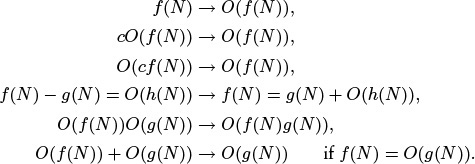
Some of the basic manipulations that we use when working with expressions containing the O-notation are the subject of Exercises 2.20 through 2.25. Many of these manipulations are intuitive, but mathematically inclined readers may be interested in working Exercise 2.21 to prove the validity of the basic operations from the definition. Essentially, these exercises say that we can expand algebraic expressions using the O-notation as though the O were not there, then can drop all but the largest term. For example, if we expand the expression
(N + O(1))(N + O (log N) + O(1)),
we get six terms
N2 + O(N) + O(N log N) + O(log N) + O(N) + O(1),
but can drop all but the largest O-term, leaving the approximation
N2 + O(N log N).
That is, N2 is a good approximation to this expression when N is large. These manipulations are intuitive, but the O-notation allows us to express them mathematically with rigor and precision. We refer to a formula with one O-term as an asymptotic expression.
For a more relevant example, suppose that (after some mathematical analysis) we determine that a particular algorithm has an inner loop that is iterated 2NHN times on the average, an outer section that is iterated N times, and some initialization code that is executed once. Suppose further that we determine (after careful scrutiny of the implementation) that each iteration of the inner loop requires a0 nanoseconds, the outer section requires a1 nanoseconds, and the initialization part a2 nanoseconds. Then we know that the average running time of the program (in nanoseconds) is
2a0NHN + a1N + a2.
But it is also true that the running time is
2a0NHN + O(N).
This simpler form is significant because it says that, for large N, we may not need to find the values of a1 or a2 to approximate the running time. In general, there could well be many other terms in the mathematical expression for the exact running time, some of which may be difficult to analyze. The O-notation provides us with a way to get an approximate answer for large N without bothering with such terms.
Continuing this example, we also can use the O-notation to express running time in terms of a familiar function, ln N. In terms of the O-notation, the approximation in Table 2.3 is expressed as HN = ln N + O(1). Thus, 2a0N ln N + O(N) is an asymptotic expression for the total running time of our algorithm. We expect the running time to be close to the easily computed value 2a0N ln N for large N. The constant factor a0 depends on the time taken by the instructions in the inner loop.
Furthermore, we do not need to know the value of a0 to predict that the running time for input of size 2N will be about twice the running time for input of size N for huge N because
That is, the asymptotic formula allows us to make accurate predictions without concerning ourselves with details of either the implementation or the analysis. Note that such a prediction would not be possible if we were to have only an O-approximation for the leading term.
The kind of reasoning just outlined allows us to focus on the leading term when comparing or trying to predict the running times of algorithms. We are so often in the position of counting the number of times that fixed-cost operations are performed and wanting to use the leading term to estimate the result that we normally keep track of only the leading term, assuming implicitly that a precise analysis like the one just given could be performed, if necessary.
When a function f(N) is asymptotically large compared to another function g(N) (that is, g(N)/f(N) → 0 as N → ∞), we sometimes use in this book the (decidedly nontechnical) terminology about f(N) to mean f(N)+O(g(N)). What we seem to lose in mathematical precision we gain in clarity, for we are more interested in the performance of algorithms than in mathematical details. In such cases, we can rest assured that, for large N (if not for all N), the quantity in question will be close to f(N). For example, even if we know that a quantity is N(N – 1)/2, we may refer to it as being about N2/2. This way of expressing the result is more quickly understood than the more detailed exact result, and, for example, deviates from the truth only by 0.1 percent for N = 1000. The precision lost in such cases pales by comparison with the precision lost in the more common usage O(f(N)). Our goal is to be both precise and concise when describing the performance of algorithms.
In a similar vein, we sometimes say that the running time of an algorithm is proportional to f(N) when we can prove that it is equal to cf(N)+g(N) with g(N) asymptotically smaller than f(N). When this kind of bound holds, we can project the running time for, say, 2N from our observed running time for N, as in the example just discussed. Figure 2.5 gives the factors that we can use for such projection for functions that commonly arise in the analysis of algorithms. Coupled with empirical studies (see Section 2.1), this approach frees us from the task of determining implementation-dependent constants in detail. Or, working backward, we often can easily develop an hypothesis about the functional growth of the running time of a program by determining the effect of doubling N on running time.
The distinctions among O-bounds, is proportional to, and about are illustrated in Figures 2.3 and 2.4. We use O-notation primarily to learn the fundamental asymptotic behavior of an algorithm; is proportional to when we want to predict performance by extrapolation from empirical studies; and about when we want to compare performance or to make absolute performance predictions.
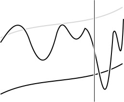
In this schematic diagram, the oscillating curve represents a function, g(N), which we are trying to approximate; the black smooth curve represents another function, f(N), which we are trying to use for the approximation; and the gray smooth curve represents cf(N) for some unspecified constant c. The vertical line represents a value N0, indicating that the approximation is to hold for N > N0. When we say that g(N) = O(f(N)), we expect only that the value of g(N) falls below some curve the shape of f(N) to the right of some vertical line. The behavior of f(N) could otherwise be erratic (for example, it need not even be continuous).
Figure 2.3 Bounding a function with an O-approximation
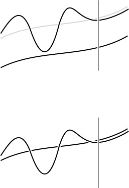
When we say that g(N) is proportional to f(N) (top), we expect that it eventually grows like f(N) does, but perhaps offset by an unknown constant. Given some value of g(N), this knowledge allows us to estimate it for larger N. When we say that g(N) is about f(N) (bottom), we expect that we can eventually use f to estimate the value of g accurately.
Figure 2.4 Functional approximations
2.21 Prove that we can make any of the following transformations in an expression that uses the O-notation:
![]() 2.22 Show that (N + 1)(HN + O(1)) = N ln N + O(N).
2.22 Show that (N + 1)(HN + O(1)) = N ln N + O(N).
2.23 Show that N ln N = O(N3/2).
![]() 2.24 Show that NM = O(αN) for any M and any constant α > 1.
2.24 Show that NM = O(αN) for any M and any constant α > 1.
2.26 Suppose that Hk = N. Give an approximate formula that expresses k as a function of N.
![]() 2.27 Suppose that lg(k!) = N. Give an approximate formula that expresses k as a function of N.
2.27 Suppose that lg(k!) = N. Give an approximate formula that expresses k as a function of N.
![]() 2.28 You are given the information that the running time of one algorithm is O(N log N) and that the running time of another algorithm is O(N3). What does this statement imply about the relative performance of the algorithms?
2.28 You are given the information that the running time of one algorithm is O(N log N) and that the running time of another algorithm is O(N3). What does this statement imply about the relative performance of the algorithms?
![]() 2.29 You are given the information that the running time of one algorithm is always about N log N and that the running time of another algorithm is O(N3). What does this statement imply about the relative performance of the algorithms?
2.29 You are given the information that the running time of one algorithm is always about N log N and that the running time of another algorithm is O(N3). What does this statement imply about the relative performance of the algorithms?
![]() 2.30 You are given the information that the running time of one algorithm is always about N log N and that the running time of another algorithm is always about N3. What does this statement imply about the relative performance of the algorithms?
2.30 You are given the information that the running time of one algorithm is always about N log N and that the running time of another algorithm is always about N3. What does this statement imply about the relative performance of the algorithms?
![]() 2.31 You are given the information that the running time of one algorithm is always proportional to N log N and that the running time of another algorithm is always proportional to N3. What does this statement imply about the relative performance of the algorithms?
2.31 You are given the information that the running time of one algorithm is always proportional to N log N and that the running time of another algorithm is always proportional to N3. What does this statement imply about the relative performance of the algorithms?
![]() 2.32 Derive the factors given in Figure 2.5: For each function f(N) that appears on the left, find an asymptotic formula for f(2N)/f(N).
2.32 Derive the factors given in Figure 2.5: For each function f(N) that appears on the left, find an asymptotic formula for f(2N)/f(N).
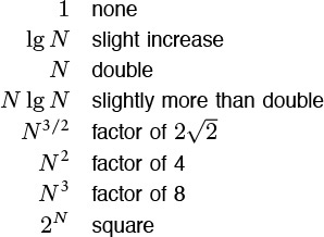
Predicting the effect of doubling the problem size on the running time is a simple task when the running time is proportional to certain simple functions, as indicated in this table. In theory, we cannot depend on this effect unless N is huge, but this method is surprisingly effective. Conversely, a quick method for determining the functional growth of the running time of a program is to run that program empirically, doubling the input size for N as large as possible, then work backward from this table.
Figure 2.5 Effect of doubling problem size on running time
2.5 Basic Recurrences
As we shall see throughout the book, a great many algorithms are based on the principle of recursively decomposing a large problem into one or more smaller ones, using solutions to the subproblems to solve the original problem. We discuss this topic in detail in Chapter 5, primarily from a practical point of view, concentrating on implementations and applications. We also consider an example in detail in Section 2.6. In this section, we look at basic methods for analyzing such algorithms and derive solutions to a few standard formulas that arise in the analysis of many of the algorithms that we will be studying. Understanding the mathematical properties of the formulas in this section will give us insight into the performance properties of algorithms throughout the book.
Formula 2.1 This formula arises for a program that loops through the input to eliminate one item:
CN = CN–1 + N, for N ≥ 2 with C1 = 1.
Solution: CN is about N2/2. To find the value of CN, we telescope the equation by applying it to itself, as follows:
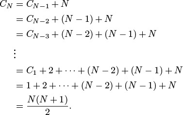
Evaluating the sum 1 + 2 + ··· + (N – 2) + (N – 1) + N is elementary: The given result follows when we add the sum to itself, but in reverse order, term by term. This result—twice the value sought—consists of N terms, each of which sums to N + 1.
This simple example illustrates the basic scheme that we use in this section as we consider a number of formulas, which are all based on the principle that recursive decomposition in an algorithm is directly reflected in its analysis. For example, the running time of such algorithms is determined by the size and number of the subproblems and the time required for the decomposition. Mathematically, the dependence of the running time of an algorithm for an input of size N on its running time for smaller inputs is captured easily with formulas called recurrence relations. Such formulas describe precisely the performance of the corresponding algorithms: To derive the running time, we solve the recurrences. More rigorous arguments related to specific algorithms will come up when we get to the algorithms—here, we concentrate on the formulas themselves.
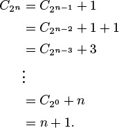
Formula 2.2 This recurrence arises for a recursive program that halves the input in one step:
CN = CN/2 + 1, for N ≥ 2 with C1 = 1.
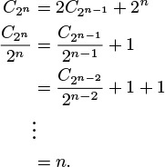
Solution: CN is about lg N. As written, this equation is meaningless unless N is even or we assume that N/2 is an integer division. For the moment, we assume that N = 2n, so the recurrence is always well-defined. (Note that n = lg N.) But then the recurrence telescopes even more easily than our first recurrence:
The precise solution for general N depends on the interpretation of N/2. In the case that N/2 represents ![]() N/2
N/2![]() , we have a simple solution: CN is the number of bits in the binary representation of N, and that number is
, we have a simple solution: CN is the number of bits in the binary representation of N, and that number is ![]() lg N
lg N![]() + 1, by definition. This conclusion follows immediately from the fact that the operation of eliminating the rightmost bit of the binary representation of any integer N > 0 converts it into
+ 1, by definition. This conclusion follows immediately from the fact that the operation of eliminating the rightmost bit of the binary representation of any integer N > 0 converts it into ![]() N/2
N/2![]() (see Figure 2.6).
(see Figure 2.6).

Given the binary representation of a number N (center), we obtain ![]() N/2
N/2![]() by removing the rightmost bit. That is, the number of bits in the binary representation of N is 1 greater than the number of bits in the binary representation of
by removing the rightmost bit. That is, the number of bits in the binary representation of N is 1 greater than the number of bits in the binary representation of ![]() N/2
N/2![]() . Therefore,
. Therefore, ![]() lg N
lg N![]() + 1, the number of bits in the binary representation of N, is the solution to Formula 2.2 for the case that N/2 is interpreted as
+ 1, the number of bits in the binary representation of N, is the solution to Formula 2.2 for the case that N/2 is interpreted as ![]() N/2
N/2![]() .
.
Figure 2.6 Integer functions and binary representations
Formula 2.3 This recurrence arises for a recursive program that halves the input, but perhaps must examine every item in the input.
CN = CN/2 + N, for N ≥ 2 with C1 = 0.
Solution: CN is about 2N. The recurrence telescopes to the sum N + N/2 + N/4 + N/8 + ... . (Like Formula 2.2, the recurrence is precisely defined only when N is a power of 2). If the sequence is infinite, this simple geometric sum evaluates to exactly 2N. Because we use integer division and stop at 1, this value is an approximation to the exact answer. The precise solution involves properties of the binary representation of N.
Formula 2.4 This recurrence arises for a recursive program that has to make a linear pass through the input, before, during, or after splitting that input into two halves:
CN = 2CN/2 + N, for N ≥ 2 with C1 = 0.
Solution: CN is about N lg N. This solution is the most widely cited of those we are considering here, because the recurrence applies to a family of standard divide-and-conquer algorithms.
We develop the solution very much as we did in Formula 2.2, but with the additional trick of dividing both sides of the recurrence by 2n at the second step to make the recurrence telescope.
Formula 2.5 This recurrence arises for a recursive program that splits the input into two halves and then does a constant amount of other work (see Chapter 5).
CN = 2CN/2 + 1, for N ≥ 2 with C1 = 1.
Solution: CN is about 2N. We can derive this solution in the same manner as we did the solution to Formula 2.4.
We can solve minor variants of these formulas, involving different initial conditions or slight differences in the additive term, using the same solution techniques, although we need to be aware that some recurrences that seem similar to these may actually be rather difficult to solve. There is a variety of advanced general techniques for dealing with such equations with mathematical rigor (see reference section). We will encounter a few more complicated recurrences in later chapters, but we defer discussion of their solution until they arise.
Exercises
![]() 2.33 Give a table of the values of CN in Formula 2.2 for 1 ≤ N ≤ 32, interpreting N/2 to mean
2.33 Give a table of the values of CN in Formula 2.2 for 1 ≤ N ≤ 32, interpreting N/2 to mean ![]() N/2
N/2![]() .
.
![]() 2.34 Answer Exercise 2.33, but interpret N/2 to mean
2.34 Answer Exercise 2.33, but interpret N/2 to mean ![]() N/2
N/2![]() .
.
![]() 2.35 Answer Exercise 2.34 for Formula 2.3.
2.35 Answer Exercise 2.34 for Formula 2.3.
![]() 2.36 Suppose that fN is proportional to a constant and that
2.36 Suppose that fN is proportional to a constant and that
CN = CN/2 + fN, for N ≥ t with 0 ≤ CN < c for N < t,
where c and t are both constants. Show that CN is proportional to lg N.
![]() 2.37 State and prove generalized versions of Formulas 2.3 through 2.5 that are analogous to the generalized version of Formula 2.2 in Exercise 2.36.
2.37 State and prove generalized versions of Formulas 2.3 through 2.5 that are analogous to the generalized version of Formula 2.2 in Exercise 2.36.
2.38 Give a table of the values of CN in Formula 2.4 for 1 ≤ N ≤ 32, for the following three cases: (i) interpret N/2 to mean ![]() N/2
N/2![]() ; (ii) interpret N/2 to mean
; (ii) interpret N/2 to mean ![]() N/2
N/2![]() ; (iii) interpret 2CN/2 to mean C
; (iii) interpret 2CN/2 to mean C![]() N/2
N/2![]() + C
+ C![]() N/2
N/2![]() .
.
2.39 Solve Formula 2.4 for the case when N/2 is interpreted as ![]() N/2
N/2![]() , by using a correspondence to the binary representation of N, as in the proof of Formula 2.2. Hint: Consider all the numbers less than N.
, by using a correspondence to the binary representation of N, as in the proof of Formula 2.2. Hint: Consider all the numbers less than N.
CN = CN/2 + N2, for N ≥ 2 with C1 = 0,
when N is a power of 2.
CN = CN/α + 1, for N ≥ 2 with C1 = 0,
when N is a power of α.
CN = αCN/2, for N ≥ 2 with C1 = 1,
when N is a power of 2.
CN = (CN/2)2, for N ≥ 2 with C1 = 1,
when N is a power of 2.
when N is a power of 2.
![]() 2.45 Consider the family of recurrences like Formula 2.1, where we allow N/2 to be interpreted as
2.45 Consider the family of recurrences like Formula 2.1, where we allow N/2 to be interpreted as ![]() N/2
N/2![]() or
or ![]() N/2
N/2![]() , and we require only that the recurrence hold for N > c0 with CN = O(1) for N ≤ c0. Prove that lg N + O(1) is the solution to all such recurrences.
, and we require only that the recurrence hold for N > c0 with CN = O(1) for N ≤ c0. Prove that lg N + O(1) is the solution to all such recurrences.
![]() 2.46 Develop generalized recurrences and solutions similar to Exercise 2.45 for Formulas 2.2 through 2.5.
2.46 Develop generalized recurrences and solutions similar to Exercise 2.45 for Formulas 2.2 through 2.5.
2.6 Examples of Algorithm Analysis
Armed with the tools outlined in the previous three sections, we now consider the analysis of sequential search and binary search, two basic algorithms for determining whether or not any of a sequence of objects appears among a set of previously stored objects. Our purpose is to illustrate the manner in which we will compare algorithms, rather than to describe these particular algorithms in detail. For simplicity, we assume here that the objects in question are integers. We will consider more general applications in great detail in Chapters 12 through 16. The simple versions of the algorithms that we consider here not only expose many aspects of the algorithm design and analysis problem, but also have many direct applications.
For example, we might imagine a credit-card company that has N credit risks or stolen credit cards, and that wants to check whether any of M given transactions involves any one of the N bad numbers. To be concrete, we might think of N being large (say on the order of 103 to 106) and M being huge (say on the order of 106 to 109) for this application. The goal of the analysis is to be able to estimate the running times of the algorithms when the values of the parameters fall within these ranges.
Program 2.1 implements a straightforward solution to the search problem. It is packaged as a C function that operates on an array (see Chapter 3) for better compatibility with other code that we will examine for the same problem in Part 4, but it is not necessary to understand the details of the packaging to understand the algorithm: We store all the objects in an array; then, for each transaction, we look through the array sequentially, from beginning to end, checking each to see whether it is the one that we seek.
To analyze the algorithm, we note immediately that the running time depends on whether or not the object sought is in the array. We can determine that the search is unsuccessful only by examining each of the N objects, but a search could end successfully at the first, second, or any one of the objects.
Therefore, the running time depends on the data. If all the searches are for the number that happens to be in the first position in the array, then the algorithm will be fast; if they are for the number that happens to be in the last position in the array, it will be slow. We discuss in Section 2.7 the distinction between being able to guarantee performance and being able to predict performance. In this case, the best guarantee that we can provide is that no more that N numbers will be examined.
To make a prediction, however, we need to make an assumption about the data. In this case, we might choose to assume that all the numbers are randomly chosen. This assumption implies, for example, that each number in the table is equally likely to be the object of a search. On reflection, we realize that it is that property of the search that is critical, because with randomly chosen numbers we would be unlikely to have a successful search at all (see Exercise 2.48). For some applications, the number of transactions that involve a successful search might be high; for other applications, it might be low. To avoid confusing the model with properties of the application, we separate the two cases (successful and unsuccessful) and analyze them independently. This example illustrates that a critical part of an effective analysis is the development of a reasonable model for the application at hand. Our analytic results will depend on the proportion of searches that are successful; indeed, it will give us information that we might need if we are to choose different algorithms for different applications based on this parameter.
Property 2.1 Sequential search examines N numbers for each unsuccessful search and about N/2 numbers for each successful search on the average.
If each number in the table is equally likely to be the object of a search, then
(1 + 2 + ... + N)/N = (N + 1)/2
is the average cost of a search. ![]()
Property 2.1 implies that the running time of Program 2.1 is proportional to N, subject to the implicit assumption that the average cost of comparing two numbers is constant. Thus, for example, we can expect that, if we double the number of objects, we double the amount of time required for a search.
We can speed up sequential search for unsuccessful search by putting the numbers in the table in order. Sorting the numbers in the table is the subject of Chapters 6 through 11. A number of the algorithms that we will consider get that task done in time proportional to N log N, which is insignificant by comparison to the search costs when M is huge. In an ordered table, we can terminate the search immediately on reaching a number that is larger than the one that we seek. This change reduces the cost of sequential search to about N/2 numbers examined for unsuccessful search, the same as for successful search.
Property 2.2 Sequential search in an ordered table examines N numbers for each search in the worst case and about N/2 numbers for each search on the average.
We still need to specify a model for unsuccessful search. This result follows from assuming that the search is equally likely to terminate at any one of the N + 1 intervals defined by the N numbers in the table,
which leads immediately to the expression
(1 + 2 + ... + N + N)/N = (N + 3)/2.
The cost of an unsuccessful search ending before or after the Nth entry in the table is the same: N. ![]()
Another way to state the result of Property 2.2 is to say that the running time of sequential search is proportional to MN for M transactions, on the average and in the worst case. If we double either the number of transactions or the number of objects in the table, we can expect the running time to double; if we double both, we can expect the running time to go up by a factor of 4. The result also tells us that the method is not suitable for huge tables. If it takes c microseconds to examine a single number, then, for M = 109 and N = 106, the running time for all the transactions would be at least (c/2)109 seconds, or, by Figure 2.1, about 16c years, which is prohibitive.
Program 2.2 is a classical solution to the search problem that is much more efficient than sequential search. It is based on the idea that, if the numbers in the table are in order, we can eliminate half of them from consideration by comparing the one that we seek with the one at the middle position in the table. If it is equal, we have a successful search. If it is less, we apply the same method to the left half of the table. If it is greater, we apply the same method to the right half of the table. Figure 2.7 is an example of the operation of this method on a sample set of numbers.

To see whether or not 5025 is in the table of numbers in the left column, we first compare it with 6504; that leads us to consider the first half of the array. Then we compare against 4548 (the middle of the first half); that leads us to the second half of the first half. We continue, always working on a subarray that would contain the number being sought, if it is in the table. Eventually, we get a subarray with just 1 element, which is not equal to 5025, so 5025 is not in the table.
Figure 2.7 Binary search
Property 2.3 Binary search never examines more than ![]() lg N
lg N![]() + 1 numbers.
+ 1 numbers.
The proof of this property illustrates the use of recurrence relations in the analysis of algorithms. If we let TN represent the number of comparisons required for binary search in the worst case, then the way in which the algorithm reduces search in a table of size N to search in a table half the size immediately implies that
TN ≤ T ![]() N/2
N/2![]() + 1, for N ≥ 2 with T1 = 1.
+ 1, for N ≥ 2 with T1 = 1.
To search in a table of size N, we examine the middle number, then search in a table of size no larger than ![]() N/2
N/2![]() . The actual cost could be less than this value because the comparison might cause us to terminate a successful search, or because the table to be searched might be of size
. The actual cost could be less than this value because the comparison might cause us to terminate a successful search, or because the table to be searched might be of size ![]() N/2
N/2![]() – 1 (if N is even). As we did in the solution of Formula 2.2, we can prove immediately that TN ≤ n + 1 if N = 2n and then verify the general result by induction.
– 1 (if N is even). As we did in the solution of Formula 2.2, we can prove immediately that TN ≤ n + 1 if N = 2n and then verify the general result by induction. ![]()
Property 2.3 allows us to solve a huge search problem with up to 1 million numbers with at most 20 comparisons per transaction, and that is likely to be less than the time it takes to read or write the number on many computers. The search problem is so important that several methods have been developed that are even faster than this one, as we shall see in Chapters 12 through 16.
Note that we express Property 2.1 and Property 2.2 in terms of the operations that we perform most often on the data. As we noted in the commentary following Property 2.1, we expect that each operation should take a constant amount of time, and we can conclude that the running time of binary search is proportional to lg N as compared to N for sequential search. As we double N, the running time of binary search hardly changes, but the running time of sequential search doubles. As N grows, the gap between the two methods becomes a chasm.
We can verify the analytic evidence of Properties 2.1 and 2.2 by implementing and testing the algorithms. For example, Table 2.4 shows running times for binary search and sequential search for M searches in a table of size N (including, for binary search, the cost of sorting the table) for various values of M and N. We will not consider the implementation of the program to run these experiments in detail here because it is similar to those that we consider in full detail in Chapters 6 and 11, and because we consider the use of library and external functions and other details of putting together programs from constituent pieces, including the sort function, in Chapter 3. For the moment, we simply stress that doing empirical testing is an integral part of evaluating the efficiency of an algorithm.
These relative timings validate our analytic results that sequential search takes time proportional to MN and binary search takes time proportional to M lg N for M searches in a table of N objects. When we increase N by a factor of 2, the time for sequential search increases by a factor of 2 as well, but the time for binary search hardly changes. Sequential search is infeasible for huge M as N increases, but binary search is fast even for huge tables.
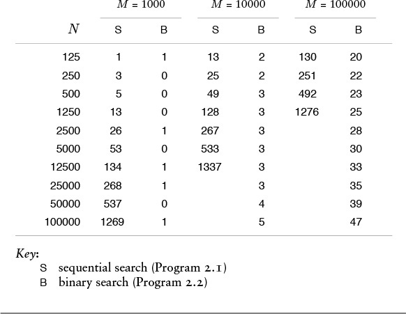
Table 2.4 Empirical study of sequential and binary search
Table 2.4 validates our observation that the functional growth of the running time allows us to predict performance for huge cases on the basis of empirical studies for small cases. The combination of mathematical analysis and empirical studies provides persuasive evidence that binary search is the preferred algorithm, by far.
This example is a prototype of our general approach to comparing algorithms. We use mathematical analysis of the frequency with which algorithms perform critical abstract operations, then use those results to deduce the functional form of the running time, which allows us to verify and extend empirical studies. As we develop algorithmic solutions to computational problems that are more and more refined, and as we develop mathematical analyses to learn their performance characteristics that are more and more refined, we call on mathematical studies from the literature, so as to keep our attention on the algorithms themselves in this book. We cannot do thorough mathematical and empirical studies of every algorithm that we encounter, but we strive to identify essential performance characteristics, knowing that, in principle, we can develop a scientific basis for making informed choices among algorithms in critical applications.
Exercises
![]() 2.47 Give the average number of comparisons used by Program 2.1 in the case that αN of the searches are successful, for 0 ≤ α ≤ 1.
2.47 Give the average number of comparisons used by Program 2.1 in the case that αN of the searches are successful, for 0 ≤ α ≤ 1.
![]() 2.48 Estimate the probability that at least one of M random 10-digit numbers matches one of a set of N given values, for M = 10, 100, and 1000 and N = 103, 104, 105, and 106.
2.48 Estimate the probability that at least one of M random 10-digit numbers matches one of a set of N given values, for M = 10, 100, and 1000 and N = 103, 104, 105, and 106.
2.49 Write a driver program that generates M random integers and puts them in an array, then counts the number of N random integers that matches one of the numbers in the array, using sequential search. Run your program for M = 10, 100, and 1000 and N = 10, 100, and 1000.
![]() 2.50 State and prove a property analogous to Property 2.3 for binary search.
2.50 State and prove a property analogous to Property 2.3 for binary search.
2.7 Guarantees, Predictions, and Limitations
The running time of most algorithms depends on their input data. Typically, our goal in the analysis of algorithms is somehow to eliminate that dependence: We want to be able to say something about the performance of our programs that depends on the input data to as little an extent as possible, because we generally do not know what the input data will be each time the program is invoked. The examples in Section 2.6 illustrate the two major approaches that we use toward this end: worst-case analysis and average-case analysis.
Studying the worst-case performance of algorithms is attractive because it allows us to make guarantees about the running time of programs. We say that the number of times certain abstract operations are executed is less than a certain function of the number of inputs, no matter what the input values are. For example, Property 2.3 is an example of such a guarantee for binary search, as is Property 1.3 for weighted quick union. If the guarantees are low, as is the case with binary search, then we are in a favorable situation, because we have eliminated cases for which our program might run slowly. Programs with good worst-case performance characteristics are a basic goal in algorithm design.
There are several difficulties with worst-case analysis, however. For a given algorithm, there might be a significant gap between the time required for it to solve a worst-case instance of the input and the time required for it to solve the data that it might encounter in practice. For example, quick union requires time proportional to N in the worst case, but only log N for typical data. More important, we cannot always prove that there is an input for which the running time of an algorithm achieves a certain bound; we can prove only that it is guaranteed to be lower than the bound. Moreover, for some problems, algorithms with good worst-case performance are significantly more complicated than are other algorithms. We often find ourselves in the position of having an algorithm with good worst-case performance that is slower than simpler algorithms for the data that occur in practice, or that is not sufficiently faster that the extra effort required to achieve good worst-case performance is justified. For many applications, other considerations—such as portability or reliability—are more important than improved worst-case performance guarantees. For example, as we saw in Chapter 1, weighted quick union with path compression provides provably better performance guarantees than weighted quick union, but the algorithms have about the same running time for typical practical data.
Studying the average-case performance of algorithms is attractive because it allows us to make predictions about the running time of programs. In the simplest situation, we can characterize precisely the inputs to the algorithm; for example, a sorting algorithm might operate on an array of N random integers, or a geometric algorithm might process a set of N random points in the plane with coordinates between 0 and 1. Then, we calculate the average number of times that each instruction is executed, and calculate the average running time of the program by multiplying each instruction frequency by the time required for the instruction and adding them all together.
There are also several difficulties with average-case analysis, however. First, the input model may not accurately characterize the inputs encountered in practice, or there may be no natural input model at all. Few people would argue against the use of input models such as “randomly ordered file” for a sorting algorithm, or “random point set” for a geometric algorithm, and for such models it is possible to derive mathematical results that can predict accurately the performance of programs running on actual applications. But how should one characterize the input to a program that processes English-language text? Even for sorting algorithms, models other than randomly ordered inputs are of interest in certain applications. Second, the analysis might require deep mathematical reasoning. For example, the average-case analysis of union-find algorithms is difficult. Although the derivation of such results is normally beyond the scope of this book, we will illustrate their nature with a number of classical examples, and we will cite relevant results when appropriate (fortunately, many of our best algorithms have been analyzed in the research literature). Third, knowing the average value of the running time might not be sufficient: we may need to know the standard deviation or other facts about the distribution of the running time, which may be even more difficult to derive. In particular, we are often interested in knowing the chance that the algorithm could be dramatically slower than expected.
In many cases, we can answer the first objection listed in the previous paragraph by turning randomness to our advantage. For example, if we randomly scramble an array before attempting to sort it, then the assumption that the elements in the array are in random order is accurate. For such algorithms, which are called randomized algorithms, the average-case analysis leads to predictions of the expected running time in a strict probabilistic sense. Moreover, we are often able to prove that the probability that such an algorithm will be slow is negligibly small. Examples of such algorithms include quicksort (see Chapter 9), randomized BSTs (see Chapter 13), and hashing (see Chapter 14).
The field of computational complexity is the branch of analysis of algorithms that helps us to understand the fundamental limitations that we can expect to encounter when designing algorithms. The overall goal is to determine the worst-case running time of the best algorithm to solve a given problem, to within a constant factor. This function is called the complexity of the problem.
Worst-case analysis using the O-notation frees the analyst from considering the details of particular machine characteristics. The statement that the running time of an algorithm is O(f(N)) is independent of the input and is a useful way to categorize algorithms in a way that is independent of both inputs and implementation details, separating the analysis of an algorithm from any particular implementation. We ignore constant factors in the analysis; in most cases, if we want to know whether the running time of an algorithm is proportional to N or proportional to log N, it does not matter whether the algorithm is to be run on a nanocomputer or on a supercomputer, and it does not matter whether the inner loop has been implemented carefully with only a few instructions or badly implemented with many instructions.
When we can prove that the worst-case running time of an algorithm to solve a certain problem is O(f(N)), we say that f(N) is an upper bound on the complexity of the problem. In other words, the running time of the best algorithm to solve a problem is no higher than the running time of any particular algorithm to solve the problem.
We constantly strive to improve our algorithms, but we eventually reach a point where no change seems to improve the running time. For every given problem, we are interested in knowing when to stop trying to find improved algorithms, so we seek lower bounds on the complexity. For many problems, we can prove that any algorithm to solve the problem must use a certain number of fundamental operations. Proving lower bounds is a difficult matter of carefully constructing a machine model and then developing intricate theoretical constructions of inputs that are difficult for any algorithm to solve. We rarely touch on the subject of proving lower bounds, but they represent computational barriers that guide us in the design of algorithms, so we maintain awareness of them when they are relevant.
When complexity studies show that the upper bound of an algorithm matches the lower bound, then we have some confidence that it is fruitless to try to design an algorithm that is fundamentally faster than the best known, and we can start to concentrate on the implementation. For example, binary search is optimal, in the sense that no algorithm that uses comparisons exclusively can use fewer comparisons in the worst case than binary search.
We also have matching upper and lower bounds for pointer-based union-find algorithms. Tarjan showed in 1975 that weighted quick union with path compression requires following less than O(lg* V) pointers in the worst case, and that any pointer-based algorithm must follow more than a constant number of pointers in the worst case for some input. In other words, there is no point looking for some new improvement that will guarantee to solve the problem with a linear number of i = a[i] operations. In practical terms, this difference is hardly significant, because lg* V is so small; still, finding a simple linear algorithm for this problem was a research goal for many years, and Tarjan’s lower bound has allowed researchers to move on to other problems. Moreover, the story shows that there is no avoiding functions like the rather complicated log* function, because such functions are intrinsic to this problem.
Many of the algorithms in this book have been subjected to detailed mathematical analyses and performance studies far too complex to be discussed here. Indeed, it is on the basis of such studies that we are able to recommend many of the algorithms that we discuss.
Not all algorithms are worthy of such intense scrutiny; indeed, during the design process, it is preferable to work with approximate performance indicators to guide the design process without extraneous detail. As the design becomes more refined, so must the analysis, and more sophisticated mathematical tools need to be applied. Often, the design process leads to detailed complexity studies that lead to theoretical algorithms that are rather far from any particular application. It is a common mistake to assume that rough analyses from complexity studies will translate immediately into efficient practical algorithms; such assumptions can lead to unpleasant surprises. On the other hand, computational complexity is a powerful tool that tells us when we have reached performance limits in our design work and that can suggest departures in design in pursuit of closing the gap between upper and lower bounds.
In this book, we take the view that algorithm design, careful implementation, mathematical analysis, theoretical studies, and empirical analysis all contribute in important ways to the development of elegant and efficient programs. We want to gain information about the properties of our programs using any tools at our disposal, then to modify or develop new programs on the basis of that information. We will not be able to do exhaustive testing and analysis of every algorithm that we run in every programming environment on every machine, but we can use careful implementations of algorithms that we know to be efficient, then refine and compare them when peak performance is necessary. Throughout the book, when appropriate, we shall consider the most important methods in sufficient detail to appreciate why they perform well.