
Although tables act as the ultimate foundation for any application that you build, queries are very important as well. Most of the forms and reports that act as the user interface for your application are based on queries. An understanding of queries, what they are, and when and how to use them is imperative for your success as an Access application developer. This chapter teaches you the basics of working with queries. After reading this chapter, you will know how to build queries, add tables and fields to the queries that you create, sort the query output, and apply criteria to limit the data that appears in the query output. You will also be familiar with tips and tricks and important “gotchas” of working with queries.
A Select query is a stored question about the data stored in your database’s tables. Select queries are the foundation of much of what you do in Access. They underlie most of your forms and reports, allowing you to view the data you want, when you want. You use a simple Select query to define the tables and fields whose data you want to view and also to specify the criteria to limit the data the query’s output displays. A Select query is a query of a table or tables that just displays data; it doesn’t modify data in any way. More advanced Select queries are used to summarize data, supply the results of calculations, or cross-tabulate your data. You can use Action queries to add, edit, or delete data from your tables, based on selected criteria, but this chapter covers Select queries. Other types of queries are covered in Chapter 11, “Advanced Query Techniques.”
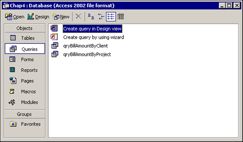
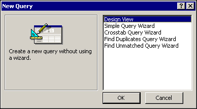
Creating a basic query is easy because Microsoft has given us a user-friendly, drag-and-drop interface. There are two ways to start a new query in Access 2002. The first way is to select the Queries icon from the Objects list in the Database window; then double-click the Create Query in Design View icon or the Create Query by Using Wizard icon. (See Figure 4.1.) The second method is to select the Queries icon from the Objects list in the Database window and then click the New command button on the Database window toolbar. The New Query dialog appears. (See Figure 4.2.) This dialog box lets you select whether you want to build the query from scratch or use one of the wizards to help you. The Simple Query Wizard walks you through the steps for creating a basic query. The other wizards help you create three specific types of queries: Crosstab, Find Duplicates, or Find Unmatched.
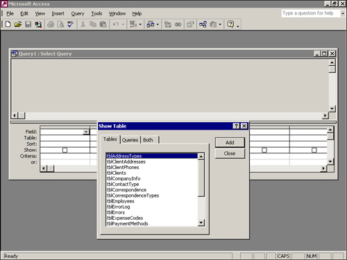
If you select Design view rather than one of the wizards, the Show Table dialog box appears. (See Figure 4.3.) Here, you can select the tables or queries that supply data to your query. Access doesn’t care whether you select tables or queries as the foundation for your queries. You can select them by double-clicking on the name of the table or query you want to add or by clicking on the table and then clicking Add. You can select multiple tables or queries by using the Shift key to select a contiguous range of tables or the Ctrl key to select noncontiguous tables. When you have selected the tables or queries you want, click Add and then click Close. This brings you to the Query Design window shown in Figure 4.4.
Tip
An alternative way to add a table is to first select Tables from the Objects list in the Database window. Then select the table on which you want the query to be based. With the table selected, select New Query from the New Object drop-down list on the toolbar or choose Query from the Insert menu. The New Query dialog appears. This is an efficient method of starting a new query based on only one table because the Show Table dialog box never appears.
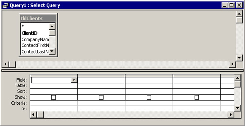
You’re now ready to select the fields you want to include in the query. The query shown in Figure 4.4 is based on the tblClients table included in the CHAP4.MDB database on the sample code CD-ROM. Notice that the query window is divided into two sections. The top half of the window shows the tables or queries that underlie the query you’re designing; the bottom half shows any fields that will be included in the query output. A field can be added to the query design grid on the bottom half of the query window in several ways:
Double-click the name of the field you want to add.
Click and drag a single field from the table in the top half of the query window to the query design grid below.
Select multiple fields at the same time by using your Shift key (for a contiguous range of fields) or your Ctrl key (for a noncontiguous range). You can double-click the title bar of the field list to select all fields; then click and drag any one of the selected fields to the query design grid.
Tip
You can double-click the asterisk to include all fields within the table in the query result. Although this is very handy, in that changes to the table structure magically affect the query’s output, I believe that this “trick” is dangerous. When the asterisk is selected, all table fields are included in the query result whether or not they are needed. This can cause major performance problems in a LAN, WAN, or client/server application.
TRY IT
Open the Northwind database that comes with Access (this database is not installed unless you designate that you want to install sample files during the install). If you want to prevent the Startup form from appearing, hold down your Shift key as you open the database. Click the Query icon and then click New. Select Design view from the New Query dialog. Add the Customers table to the query. Follow these steps to select six fields from Customers:
Hold down your Shift key and click the ContactTitle field. This should select the CustomerID, CompanyName, ContactName, and ContactTitle fields.
Scroll down the list of fields, using the vertical scrollbar, until the Region field is visible.
Hold down your Ctrl key and click the Region field.
With the Ctrl key still held down, click the Phone field. All six fields should now be selected.
Click and drag any of the selected fields from the table on the top half of the query window to the query design grid on the bottom. All six fields should appear in the query design grid. You might need to use the horizontal scrollbar to view some of the fields on the right.
Tip
The easiest way to run a query is to click the Run button on the toolbar (which looks like an exclamation point). You can click the Query View button to run a query, but this method works only for Select queries, not for Action queries. The Query View button has a special meaning for Action queries (explained in Chapter 11). Clicking Run is preferable because you don’t have to worry about what type of query you’re running. After running a Select query, you should see what looks like a datasheet, with only the fields you selected. To return to the query’s design, click the Query View button.
To remove a field from the query design grid, follow these steps:
Find the field you want to remove.
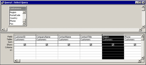
Click the small horizontal gray button (column selector) immediately above the name of the field. The entire column of the query design grid should become black. (See Figure 4.5.)
TRY IT
Assume that you have decided to remove the Region field from the query design grid. Use the horizontal scrollbar to see the Region field on the query design grid.
The process for inserting a field after a query is built differs, depending on where you want the new field to be inserted. If you want it inserted after the existing fields, it’s easiest to double-click the name of the field you want to add. If you prefer to insert the new field between two existing fields, it’s best to click and drag the field you want to add, dropping it onto the field you want to appear to the right of the inserted field.
TRY IT
To insert the Country field between the ContactTitle and Phone fields, click and drag the Country field from the table until it’s on top of the Phone field. This inserts the field in the correct place. To run the query, click Run on the toolbar.
Although the user can move a column while in a query’s Datasheet view, sometimes you want to permanently alter the position of a field in the query output. This can be done as a convenience to the user or, more importantly, because you will use the query as a foundation for forms and reports. The order of the fields in the query becomes the default order of the fields on any forms and reports you build using any of the wizards. You can save yourself quite a bit of time by ordering your queries effectively.
To move a single column, follow these steps:
Select a column while in the query’s Design view by clicking its column selector (the button immediately above the field name).
Click the selected column a second time, and then drag it to a new location on the query design grid.
Follow these steps to move more than one column at a time:
Drag across the column selectors of the columns you want to move.
Click any of the selected columns a second time, and then drag them to a new location on the query design grid.
TRY IT
Move the ContactName and ContactTitle fields so that they appear before the CompanyName field. Do this by clicking and dragging from ContactName’s column selector to ContactTitle’s column selector. Both columns should be selected. Click again on the column selector for either column, and then click and drag until the thick black line jumps to the left of the CompanyName field.
Note
Moving a column in the Datasheet view doesn’t modify the query’s underlying design. If you move a column in Datasheet view, subsequent reordering in the Design view isn’t reflected in the Datasheet view. In other words, Design view and Datasheet view are no longer synchronized, and you must reorder both by hand. This actually serves as an advantage in most cases. As you will learn later, if you want to sort by the Country field and then by the CompanyName field, the Country field must appear to the left of the CompanyName field in the design of the query. If you want the CompanyName to appear to the left of the Country in the query’s result, you must make that change in Datasheet view. The fact that the order of the columns is maintained separately in both views allows you to easily accomplish both objectives.
To save your query at any time, click the Save button on the toolbar. If the query is a new one, you’re then prompted to name your query. Query names should begin with the tag qry so that you can easily recognize and identify them as queries. It’s important to understand that, when you save a query, you’re saving only the query’s definition, not the actual query result.
Return to the design of the query. To save your work, click Save on the toolbar. When prompted for a name, call the query qryCustomers.
When you run a new query, notice that the query output appears in no particular order, but generally, you want to order it. You can do this by using the Sort row of the query design grid.
To order your query result, follow these steps:
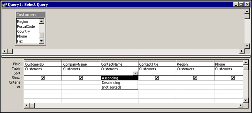
In Design view, click within the query design grid in the Sort cell of the column you want to sort. (See Figure 4.6.)
Use the drop-down combo box to select an ascending or descending sort.
TRY IT
To sort in ascending order by the ContactTitle field, follow these steps:
In Design view, click in the Sort row of the query design grid for the ContactTitle field.
Open the Sort drop-down combo box.
Select Ascending.
Run your query and view the results. Your records should now be in order by the ContactTitle field.
If you want to return to the query’s design, click View on the toolbar.
Quite often, you want to sort your query output by more than one field. The columns you want to sort must be placed in order from left to right on the query design grid, with the column you want to act as the primary sort on the far left and the secondary, tertiary, and any additional sorts following to the right. If you want the columns to appear in a different order in the query output, they need to be moved manually in Datasheet view after the query is run.
TRY IT
Sort the query output by the Country field and, within individual country groupings, by the ContactTitle field. Because sorting always occurs from left to right, you must place the Country field before the ContactTitle field. Therefore, you must move the Country field. Follow these steps:
Select the Country field from the query design grid by clicking the thin gray button above the Country column.
After you have selected the Country field, move your mouse back to the thin gray button and click and drag to the left of ContactTitle. A thick gray line should appear to the left of the ContactTitle field.
Release the mouse button.
Change the sort of the Country field to Ascending.
Run the query. The records should be in order by country and, within the country grouping, by contact title.
So far, you have learned how to select the fields you want and how to indicate the sort order for your query output. One of the important features of queries is the ability to limit your output by selection criteria. Access allows you to combine criteria by using any of several operators to limit the criteria for one or more fields. The operators and their meanings are covered in Table 4.1.
Table 4.1. Access Operators and Their Meanings
Operator | Meaning | Example | Result |
|---|---|---|---|
| Equal to |
| Finds only those records with |
| Less than |
| Finds all records with values less than 100 in that field. |
| Less than or equal to |
| Finds all records with values less than or equal to 100 in that field. |
| Greater than |
| Finds all records with values greater than 100 in that field. |
| Greater than or equal to |
| Finds all records with values greater than or equal to 100 in that field. |
| Not equal to |
| Finds all records with values other than |
| Both conditions must be true | Created by adding criteria on the same. line of the query design grid to more than one field | Finds all records where the conditions in both fields are true. |
| Either condition can be true |
| Finds all records with the value of |
| Compares a string expression to a pattern |
| Finds all records with the value of |
| Finds a range of values |
| Finds all records with the values of 5–10 (inclusive) in the field. |
| Same as |
| Finds all records with the value of |
| Same as not equal |
| Finds all records with values other than |
| Finds Nulls |
| Finds all records where no data has been entered in the field. |
| Finds all records not Null |
| Finds all records where data has been entered the field. |
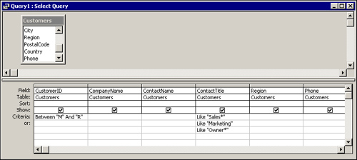
Criteria entered for two fields on a single line of the query design grid are considered an And, which means that both conditions need to be true for the record to appear in the query output. Entries made on separate lines of the query design grid are considered an Or, which means that either condition can be true for the record to be included in the query output. Take a look at the example in Figure 4.7; this query would output all records in which the ContactTitle field begins with either Marketing or Owner, regardless of the customer ID. It outputs the records in which the ContactTitle field begins with Sales only for the customers whose IDs begin with the letters M through R inclusive.
TRY IT
Design a query to find all the sales agents in Brazil or France. The criteria you build should look like those in Figure 4.8.
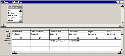
Notice that the criterion for the Country field is
"Brazil" Or "France"because you want both Brazil and France to appear in the query output. The criterion for the ContactTitle field is"Sales Agent". Because the criteria for both the Country and ContactTitle fields are entered on the same line of the query design grid, both must be true for the record to appear in the query output. In other words, the customer must be in either Brazil or France and must also be a sales agent.Modify the query so that you can output all the customers for whom the contact title begins with Sales. Try changing the criteria for the ContactTitle field to Sales. Notice that no records appear in the query output because no contact titles are just Sales. You must enter
"Like Sales*"for the criteria. Now you get the Sales Agents, Sales Associates, Sales Managers, and so on. You still don’t see the Assistant Sales Agents because their titles don’t begin with Sales. Try changing the criteria to"Like *Sales*". Now all the Assistant Sales Agents appear.
Access gives you significant power for adding date functions and expressions to your query criteria. Using these criteria, you can find all records in a certain month, on a specific weekday, or between two dates. Table 4.2 lists several examples.
Table 4.2. Sample Date Criteria
Expression | Meaning | Example | Result |
|---|---|---|---|
| Current date |
| Records with the current date within a field. |
| The day of a date |
| Records with the order date on the first day of the month. |
| The month of a date |
| Records with the order date in January. |
| The year of a date |
| Records with the order date in 1991. |
| The weekday of a date |
| Records with the order date on a Monday. |
| A range of dates |
| All records in 1995. |
| A specific part of a date |
| All records in the second quarter. |
The Weekday(Date, [FirstDayOfWeek]) function works based on your locale and how your system defines the first day of the week. Weekday() used without the optional FirstDayOfWeek argument defaults to vbSunday as the first day. A value of 0 defaults the FirstDayOfWeek to the system definition. Other values can be set also.
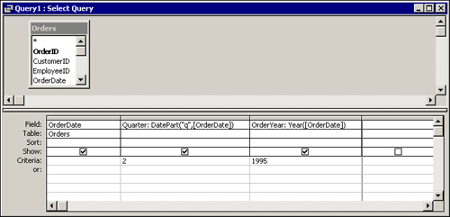
Figure 4.9 illustrates the use of a date function. Notice that DatePart("q",[OrderDate]) is entered as the expression, and the value of 2 is entered for the criteria. Year([OrderDate)] is entered as another expression with the number 1995 as the criteria. Therefore, this query outputs all records in which the order date is in the second quarter of 1995.
If you haven’t realized it yet, the results of your query can usually be updated. This means that if you modify the data in the query output, the data in the tables underlying the query is permanently modified.
Build a query based on the Customers table. Add the CustomerID, CompanyName, Address, City, and Region fields to the query design grid; then run the query. Change the address of a particular customer, and make a note of the customer ID of the customer whose address you changed. Make sure you move off the record so that the change is written to disk. Close the query, open the actual table in Datasheet view, and find the record whose address you modified. Notice that the change you made was written to the original table—this is because a query result is a dynamic set of records that maintains a link back to the original data. This happens whether you’re on a standalone machine or on a network.
Caution
It’s essential that you understand how query results are updated; otherwise, you might mistakenly update table data without even realizing you did so. Updating multitable queries is covered later in this chapter in the sections “Pitfalls of Multitable Queries” and “Row Fix-Up in Multitable Queries.”
If you have properly normalized your table data, you probably want to bring the data from your tables back together by using queries. Fortunately, you can do this quite easily with Access queries.
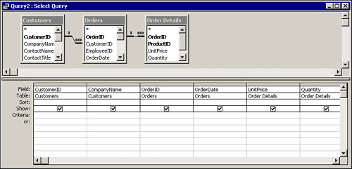
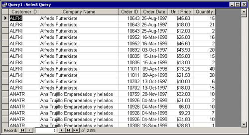
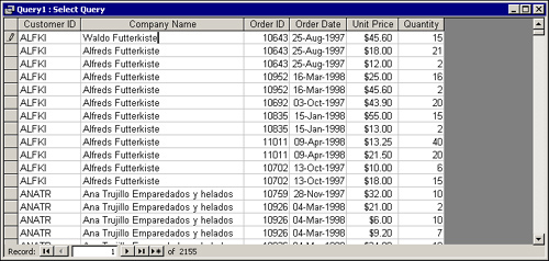
The query in Figure 4.10 joins the Customers, Orders, and Order Details tables, pulling fields from each. Notice that the CustomerID and CompanyName fields are selected from the Customers table, the OrderID and OrderDate from the Orders table, and the UnitPrice and Quantity from the Order Details table. After running this query, you should see the results shown in Figure 4.11. Notice that you get a record in the query’s result for every record in the Order Details table. In other words, there are 2,155 records in the Order Details table, and that’s how many records appear in the query output. By creating a multitable query, you can look at data from related tables, along with the data from the Order Details table.
TRY IT
Build a query that combines information from the Customers, Orders, and Order Details tables. To do this, build a new query by following these steps:
Select the Query tab from the Database window.
Click New.
Select Design view.
From the Show Table dialog box, select Customers, Orders, and Order Details by holding down the Ctrl key and clicking on each table name. Then select Add.
Click Close.
Some of the tables included in the query might be hiding below. If so, scroll down with the vertical scrollbar to view any tables that aren’t visible. Notice the join lines between the tables; they’re based on the relationships set up in the Relationships window.
Select the following fields from each table:
Customers: Country, City
Orders: Order Date
Order Details: UnitPrice, Quantity
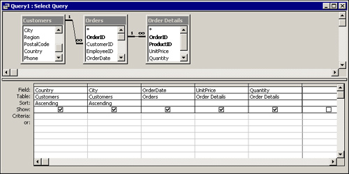
Sort by Country and then City. Your finished query design should look like the one in Figure 4.12.
Run the query. Data from all three tables should be included in the query output.
Note
To remove a table from a query, click anywhere on the table in the top half of the query design grid and press the Delete key. You can add tables to the query at any time by clicking the Show Table button from the toolbar. If you prefer, you can select the Database window and then click and drag tables directly from the Database window to the top half of the query design grid.
You should be aware of some pitfalls of multitable queries; they involve updating as well as which records you see in the query output.
It’s important to remember that certain fields in a multitable query can’t be updated. These are the join fields on the “one” side of a one-to-many relationship (unless the Cascade Update referential integrity feature has been activated). You also can’t update the join field on the “many” side of a relationship after you’ve updated data on the “one” side. More importantly, which fields can be updated, and the consequences of updating them, might surprise you. If you update the fields on the “one” side of a one-to-many relationship, you must be aware of that change’s impact. You’re actually updating that record in the original table on the “one” side of the relationship; several records on the “many” side of the relationship will be affected.
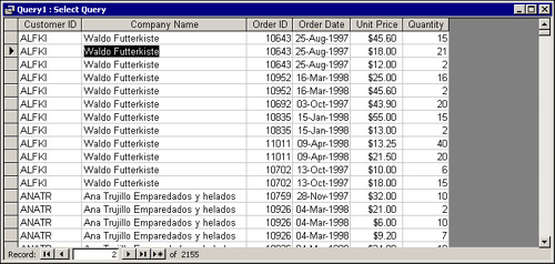
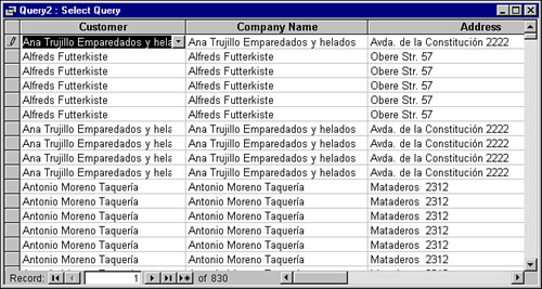
For example, Figure 4.13 shows the result of a query based on the Customers, Orders, and Order Details tables. I have changed "Alfreds Futterkiste" to "Waldo Futterkiste" on a specific record of my query output. You might expect this change to affect only that specific order detail item. Pressing the down-arrow key to move off the record shows that all records associated with Alfreds Futterkiste have been changed. (See Figure 4.14.) This happened because all the orders for Alfreds Futterkiste were actually getting their information from one record in the Customers table—the record for customer ID ALFKI. This is the record I modified while viewing the query result.
To get this experience firsthand, try changing the data in the City field for one of the records in the query result. Notice that the record (as well as several other records) is modified. This happens because the City field actually represents data from the “one” side of the one-to-many relationship. In other words, when you’re viewing the Country and City fields for several records in the query output, the data for the fields might originate from one record. The same goes for the Order Date field because it’s also on the “one” side of a one-to-many relationship. The only field in the query output that can’t be modified is TotalPrice, a calculated field. Practice modifying the data in the query result, and then returning to the original table and noticing which data has changed.
The second pitfall of multitable queries is figuring out which records result from such a query. So far, you have learned how to build only inner joins. Join types are covered in detail in Chapter 11, but for now, it’s important to understand that the query output contains only customers who have orders and orders that have order detail. This means that not all the customers or orders might be listed. In Chapter 11, you learn how to build queries in which you can list all customers, regardless of whether they have orders. You’ll also learn how to list only the customers without orders.
The row fix-up feature is automatically available to you in Access. As you fill in key values on the “many” side of a one-to-many relationship in a multitable query, the non-key values are automatically looked up in the parent table. Most database developers refer to this as enforced referential integrity. A foreign key must first exist on the “one” side of the query to be entered successfully on the “many” side. As you can imagine, you don’t want to be able to add an order to your database for a nonexistent customer.
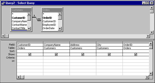
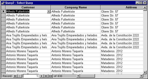
For example, the query in Figure 4.15 is based on the Customers and Orders tables. The fields included in the query are CustomerID from the Orders table; CompanyName, Address, and City from the Customers table; and OrderID and OrderDate from the Orders table. If the CustomerID associated with an order is changed, the CompanyName, Address, and City are looked up from the Customers table and immediately displayed in the query result. Notice in Figure 4.16 how the information for Alfreds Futterkiste is displayed in the query result. Figure 4.17 shows that the CompanyName, Address, and City change automatically when the CustomerID is changed. Don’t be confused by the combo box used to select the customer ID. The presence of the combo box within the query is a result of Access’s auto-lookup feature, covered in Chapter 2, “What Every Developer Needs to Know About Tables.” The customer ID associated with a particular order is actually being modified in the query. If a new record is added to the query, the customer information is filled in as soon as the customer ID associated with the order is selected.
One of the rules of data normalization is that the results of calculations shouldn’t be included in your database. You can output the results of calculations by building those calculations into your queries, and you can display the results of the calculations on forms and reports by making the query the foundation for a form or report. You can also add controls to your forms and reports containing the calculations you want. In certain cases, this can improve performance. (This topic is covered in more depth in Chapter 15, “Debugging: Your Key to Successful Development.”)
The columns of your query result can hold the result of any valid expression, including the result of a user-defined function. This makes your queries extremely powerful. For example, the following expression could be entered:
Left([FirstName],1) & "." & Left([LastName],1) & "."
This expression would give you the first character of the first name followed by a period, the first character of the last name, and another period. An even simpler expression would be this one:
[UnitPrice]*[Quantity]
This calculation would simply take the UnitPrice field and multiply it by the Quantity field. In both cases, Access would automatically name the resulting expression. For example, the calculation that results from concatenating the first and last initials is shown in Figure 4.18. Notice that in the figure, the expression has been given a name (often referred to as an “alias”). To give the expression a name, such as Initials, you must enter it as follows:
Initials:Left([FirstName],1) & "." & Left([LastName],1) & "."
![The result of the expression Initials:Left([FirstName],1) & "." & Left([LastName],1) & "." in the query.](http://imgdetail.ebookreading.net/data/2/0672321017/0672321017__alison-balters-mastering__0672321017__graphics__04fig18.jpg)
The text preceding the colon is the name of the expression—in this case, Initials. If you don’t explicitly give your expression a name, it defaults to Expr1.
TRY IT
Follow these steps to add a calculation that shows the unit price multiplied by the quantity:
Scroll to the right on the query design grid until you can see a blank column.
Click in the Field row for the new column.
Type
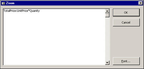
TotalPrice:UnitPrice*Quantity. If you want to see more easily what you’re typing, press Shift+F2 (Zoom). The dialog box shown in Figure 4.19 appears. (Access will supply the space after the colon and the square brackets around the field names if you omit them.)Click OK to close the Zoom window.
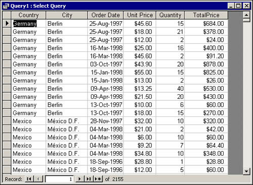
Run the query. The total sales amount should appear in the far-right column of the query output. The query output should look like the one in Figure 4.20.
Note
You can enter any valid expression in the Field row of your query design grid. Notice that field names included in an expression are automatically surrounded by square brackets, unless your field name has spaces. If a field name includes any spaces, you must enclose the field name in brackets; otherwise, your query won’t run properly. This is just one of the many reasons why field and table names shouldn’t contain spaces.
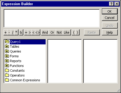
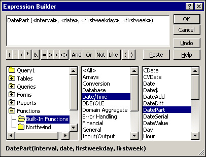
The Expression Builder is a helpful tool for building expressions in your queries, as well as in many other situations in Access. To invoke the Expression Builder, click in the Field cell of your query design grid and then click Build on the toolbar. (See Figure 4.21.) Notice that the Expression Builder is divided into three columns. The first column shows the objects in the database. After selecting an element in the left column, select the elements you want to paste from the middle and right columns.
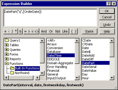
The example in Figure 4.22 shows Functions selected in the left column. Within Functions, both user-defined and built-in functions are listed; here, the Functions object is expanded with Built-In Functions selected. In the center column, Date/Time is selected. After you select Date/Time, all the built-in date and time functions appear in the right column. If you double-click a particular function—in this case, the DatePart function—the function and its parameters are placed in the text box at the top of the Expression Builder window. Notice that the DatePart function has four parameters: Interval, Date, FirstWeekDay, and FirstWeek. If you know what needs to go into each of these parameters, you can simply replace the parameter place markers with your own values. If you need more information, you can invoke help on the selected function and learn more about the required parameters. In Figure 4.23, two parameters are filled in: the interval and the name of the field being evaluated. After clicking OK, the expression is placed in the Field cell of the query.
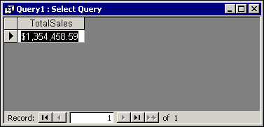
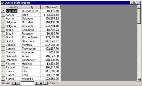
By using Totals queries, you can easily summarize numeric data. Totals queries can be used to calculate the Sum, Average, Count, Minimum, Maximum, and other types of summary calculations for the data in your query result. These queries let you calculate one value for all the records in your query result or group the calculations as desired. For example, you could determine the total sales for every record in the query result, as shown in Figure 4.24, or you could output the total sales by country and city. (See Figure 4.25.) You could also calculate the total, average, minimum, and maximum sales amounts for all customers in the United States. The possibilities are endless.
To create a Totals query, follow these steps:
Add to the query design grid the fields or expressions you want to summarize. It’s important that you add the fields in the order in which you want them grouped. For example, Figure 4.26 shows a query grouped by country, and then city.
Click Totals on the toolbar or select View|Totals to add a Total row to the query. By default, each field in the query has
Group Byin the total row.Click in the Total row on the query design grid.
Open the combo box and choose the calculation you want. (See Figure 4.26.)
Leave
Group Byin the Total cell of any fields you want to group by, as shown in Figure 4.26. Remember to place the fields in the order in which you want them grouped. For example, if you want the records grouped by country, and then by sales representative, the Country field must be placed to the left of the Sales Representative field on the query design grid. On the other hand, if you want records grouped by sales representative, and then by country, the Sales Representative field must be placed to the left of the Country field on the query design grid.Add the criteria you want to the query.
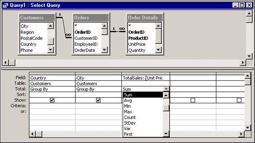
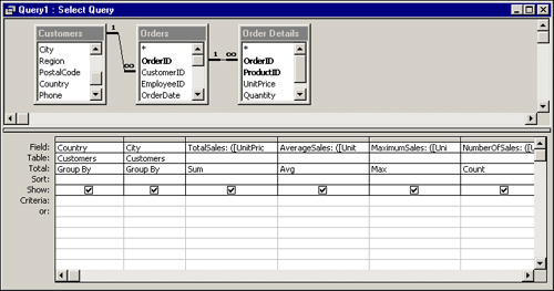
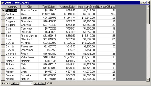
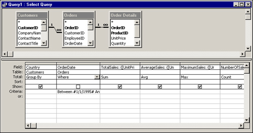
Figure 4.27 shows the design of a query that finds the total, average, maximum, and number of sales by country and city; Figure 4.28 shows the results of running the query. As you can see, Totals queries can give you valuable information.
If you save this query and reopen it, you’ll see that Access has made some changes to its design. The Total cell for the Sum is changed to Expression, and the Field cell is changed to the following:
TotalSales: Sum([UnitPrice]*[Quantity])
If you look at the Total cell for the Avg, it’s also changed to Expression. The Field cell is changed to the following:
AverageSales: Avg([UnitPrice]*[Quantity])
Access modifies the query in this way when it determines that you’re using an aggregate function on an expression having more than one field. You can enter the expression either way. Access stores and resolves the expression as noted.
TRY IT
Modify the query to show the total sales by country, city, and order date. Before you continue, save your query as qryCustomerOrderInfo, and then close it. With the Query tab of the Database window visible, click qryCustomerOrderInfo. Choose Copy from the toolbar and then Paste. Access should prompt you for the name of the new query. Type qryCustomerOrderSummary and click OK. With qryCustomerOrderSummary selected, click the Design command button. Delete both the UnitPrice and Quantity fields from the query output. To turn your query into a Totals query, follow these steps:
Click Totals on the toolbar. Notice that an extra line, called the Total line, is added to the query design grid; this line says
Group Byfor all fields.Group by country, city, and order date but total by the total price (the calculated field). Click the Total row for the TotalPrice field and use the drop-down list to select Sum. (Refer to Figure 4.26.)
Run the query. Your result should be grouped and sorted by country, city, and order date, with a total for each unique combination of the three fields.
Return to the query’s design and remove the order date from the query design grid.
Rerun the query. Notice that now you’re summarizing the query by country and city.
Change the Total row to Avg. Now you’re seeing the average price times quantity for each combination of country and city. Change it back to Sum and save the query.
As you can see, Totals queries are both powerful and flexible. Their output can’t be edited, but you can use them to view the sum, minimum, maximum, average, and count of the total price, all at the same time. You can easily modify how you’re viewing this information—by country, country and city, and so on—all at the click of your mouse.
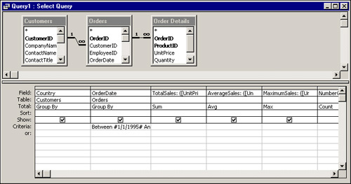
At times, you need to include a column in your query that you don’t want displayed in the query output; this is often the case with columns used solely for criteria. Figure 4.29 shows an example. If this query were run, you would get the total, average, and maximum sales grouped by both country and order date. However, you want to group only by country and use the order date only as criteria. Therefore, you need to set the Total row of the query to Where, as shown in Figure 4.30. The column used in the Where has been excluded from the query result. This is easily determined by noting that the check box in the Show row of the OrderDate column is unchecked.
Null values in your table’s fields can noticeably affect query results. A Null value is different from a zero or a zero-length string, which indicates that the data doesn’t exist for a particular field; a field contains a Null value when no value has yet been stored in the field. (As discussed in Chapter 2, a zero-length string is entered in a field by typing two quotation marks.)
Null values can affect the results of multitable queries, queries including aggregate functions (Totals queries), and queries with calculations. By default, when a multitable query is built, only records that have non-Null values on the “many” side of the relationship appear in the query result (discussed earlier in this chapter, in the “Pitfalls of Multitable Queries” section).
Null values can also affect the result of aggregate queries. For example, if you perform a count on a field containing Null values, only records having non-Null values in that field are included in the count. If you want to get an accurate count, it’s best to perform the count on a Primary Key field or some other field that can’t have Null values.
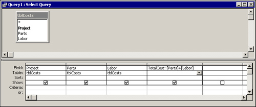
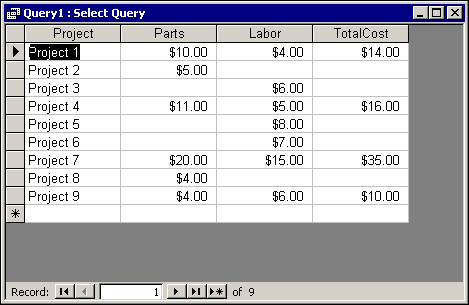
Probably the most insidious problem with Nulls happens when they’re included in calculations. A Null value, when included in a calculation containing a numeric operator (+, -, /, *, and so on), results in a Null value. In Figure 4.31, for example, notice that the query includes a calculation that adds the values in the Parts and Labor fields. These fields have been set to have no default value and, therefore, contain Nulls unless something has been explicitly entered into them. Running the query gives you the results shown in Figure 4.32. Notice that all the records having Nulls in either the Parts or Labor fields contain a Null in the result.
The solution to this problem is constructing an expression that converts the Null values to zero. The expression looks like this:
TotalCost: NZ([Parts])+NZ([Labor])
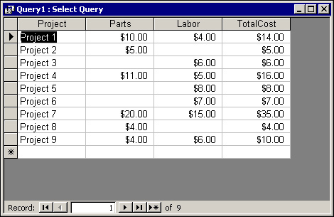
The NZ() function determines whether the Parts field contains a Null value. If the Parts field contains a Null value, it’s converted to a zero and included in the calculation; otherwise, the field’s value is used in the calculation. The same expression is used to evaluate the Labor field. The result of the modified query is shown in Figure 4.33.
Caution
Nulls really cause trouble when the results of one query containing Nulls are used in another query—a snowball effect occurs. It’s easy to miss the problem and output reports with inaccurate results. Using the NZ() function eliminates this kind of problem. You can use the NZ() function to replace the Null values with zeros or zero-length strings. Be careful when doing this, though, because it might affect other parts of your query that use this value for another calculation. Also, be sure to use any function in a query on the top level of the query tree only because functions at lower levels might hinder query performance. A query tree refers to the fact that a query can be based on other queries. Placing the criteria at the top of the query tree means that, if queries are based on other queries, the criteria should be placed in the highest-level queries.
Field and query properties can be used to refine and control the behavior and appearance of the columns in your query and of the query itself. Here’s how:
Click in a field to select the field, click in a field list to select the field list, or click in the Query Design window anywhere outside a field or the field list to select the query.
Click Properties on the toolbar.
Modify the desired property.
Note
If you click a field within the query design grid that has its Show check box cleared, only the query properties will display when you bring up the properties window for that field, not the field properties. If you mark the Show check box with the properties window open, the field properties will then be displayed.
The properties of a field in your query include the Description, Format, Input Mask, and Caption of the column. The Description property documents the use of the field and controls what appears on the status bar when the user is in that column in the query result. The Format property is the same as theq Format property in a table’s field; it controls the display of the field in the query result. The Input Mask property, like its table counterpart, actually controls how data is entered and modified in the query result. The Caption property in the query does the same thing as a Caption property of a field—sets the caption for the column in Datasheet view and the default label for forms and reports.
You might be wondering how the properties of the fields in a query interact with the same properties of a table. For example, how does the Caption property of a table’s field interact with the Caption property of the same field in a query? All properties of a table’s field are automatically inherited in your queries. Properties explicitly modified in the query override those same properties of a table’s fields. Any objects based on the query inherit the properties of the query, not those of the original table.
Note
In the case of the Input Mask property, it is important that the Input Mask in the query not be in conflict with the Input Mask of the table. The Input Mask of the query can be used to further restrict the Input Mask of the table, but not to override it. If the query’s Input Mask conflicts with the table’s Input Mask, the user will not be able to enter data into the table.
Field List properties specify attributes of each table participating in the query. The two Field List properties are Alias and Source. The Alias property is used most often when the same table is used more than once in the same query. This is done in self-joins, covered in Chapter 11. The Source property specifies a connection string or database name when you’re dealing with external tables that aren’t linked to the current database.
Microsoft offers many properties, shown in Figure 4.34, that allow you to affect the behavior of the overall query. Some of the properties are discussed here; the rest are covered as applicable throughout this book.
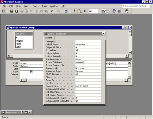
The Description property documents what the query does. The Default View property is new in Access 2002. This property determines which view will display by default whenever the query is run. Datasheet is the default setting; PivotTable or PivotChart are the other two Default View settings that are available. Output All Fields shows all the fields in the query results, regardless of the contents of the Show check box in each field. Top Values lets you specify the top x number or x percent of values in the query result. The Unique Values and Unique Records properties are used to determine whether only unique values or unique records are displayed in the query’s output. (These properties are also covered in detail in Chapter 11.)
Several other more advanced properties exist. The Run Permissions property has to do with security and is covered in Chapter 28, “Advanced Security Techniques.” Source Database, Source Connect String, ODBC Timeout, and Max Records all have to do with client/server issues and are covered in a separate book, Alison Balter’s Mastering Access 2002 Enterprise Development. The Record Locks property concerns multiuser issues and is also covered in Alison Balter’s Mastering Access 2002 Enterprise Development. The Recordset Type property determines whether updates can be made to the query output. By default, this is set to the Dynaset type allowing updates to the underlying data. Filter displays a subset that you determine, rather than the full result of the query. Order By determines the sort order of the query. The Orientation property whether the visual layout of the fields is left-to-right or right-to-left. The Subdatasheet Name property allows you to specify the name of the table or query that will appear as a subdatasheet within the current query. After the Subdatasheet property is set, the Link Child Fields and Link Master Fields properties designate the fields from the child and parent tables or queries that are used to link the current query to its subdatasheet. Finally, the Subdatasheet Height property sets the maximum height for a subdatasheet, and the Subdatasheet Expanded property determines whether the subdatasheet automatically appears in an expanded state.
You, or your application’s users, might not always know the parameters for a query output when designing the query. Parameter queries let you specify different criteria at runtime so that you don’t have to modify the query each time you want to change the criteria.
For example, say you have a query, like the one shown in Figure 4.35, for which you want users to specify the date range of the data they want to view each time they run the query. The following clause has been entered as the criteria for the OrderDate field:
Between [Enter Starting Date] And [Enter Ending Date]
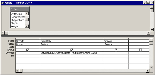
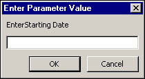
This criterion causes two dialog boxes to appear when the query is run. The first one, shown in Figure 4.36, prompts the user with the criteria text in the first set of brackets (refer to Figure 4.35). The text the user types is substituted for the bracketed text. A second dialog box appears, prompting the user for whatever is in the second set of brackets. The user’s response is used as the criterion for that query.
Add a parameter to the query qryCustomerOrderSummary so that you can view only TotalPrice summaries within a specific range. Go to the criteria for TotalPrice and type Between [Please Enter Starting Value] and [Please Enter Ending Value]. This allows you to view all the records in which the total price is within a specific range. The bracketed text is replaced by actual values when the query is run. Click OK and run the query. You’re then prompted to enter both a starting and an ending value.
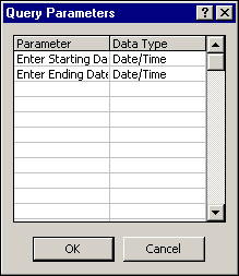
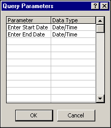
To make sure Access understands what type of data should be placed in these parameters, you must define the parameters. Do this by selecting Parameters from the Query menu to open the Parameters window. Another way to display the Query Parameters window is to right-click a gray area in the top half of the query design grid; then select Parameters from the context-sensitive, pop-up menu.
The text that appears within the brackets for each parameter must be entered in the Parameter field of the Query Parameters dialog. The type of data in the brackets must be defined in the Data Type column. Figure 4.37 shows an example of a completed Query Parameters dialog box.
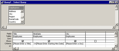
You can easily create parameters for as many fields as you want, and parameters are added just as you would add more criteria. For example, the query shown in Figure 4.38 has parameters for the Title, HireDate, and City fields in the Employees table from the Northwind database. Notice that all the criteria are on one line of the query design grid, which means that all the parameters entered must be satisfied for the records to appear in the output. The criterion for the title is [Please Enter a Title]. This means that the records in the result must match the title entered when the query is run. The criterion for the HireDate field is >=[Please Enter Starting Hire Date]. Only records with a hire date on or after the hire date entered when the query is run will appear in the output. Finally, the criterion for the City field is [Please Enter a City]. This means that only records with the City entered when the query is run will appear in the output.
The criteria for a query can also be the result of a function; this technique is covered in Chapter 11.
Note
Parameter queries offer significant flexibility; they allow the user to enter specific criteria at runtime. What’s typed in the Query Parameters dialog box must exactly match what’s typed within the brackets; otherwise, Access prompts the user with additional dialog boxes.
Tip
You can add as many parameters as you like to a query, but the user might become bothered if too many dialog boxes appear. Instead, build a custom form that feeds the Parameter query. This technique is covered in Chapter 10, “Advanced Report Techniques.”
Building Queries Needed by the Time and Billing Application for the Computer Consulting Firm
Build a query based on tblTimeCardHours. This query gives you the total billing amount by project for a specific date range. The query’s design is shown in Figure 4.39. Notice that it’s a Totals query that groups by project and totals by using the following expression:
BillAmount: Sum([BillableHours]*[BillingRate])
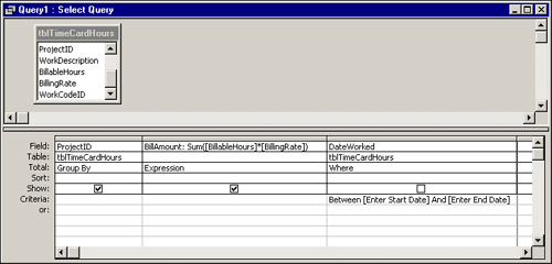
The DateWorked field is used as the Where clause for the query with this criteria:
Between [Enter Start Date] And [Enter End Date]
The two parameters of the criteria are declared in the Parameters dialog box. (See Figure 4.40.) Save this query as qryBillAmountByProject.
The second query is based on tblClients, tblProjects, and tblTimeCardHours. This query gives you the total billing amount by client for a specific date range. The query’s design is shown in Figure 4.41. This query is a Totals query that groups by the company name from the tblClients table and totals by using the following expression:
BillAmount: Sum([BillableHours]*[BillingRate])
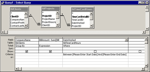
As with the first query, the DateWorked field is used as the Where clause for the query, and the parameters are defined in the Query Parameters window. Save this query as qryBillAmountByClient.
These queries are included on the sample CD-ROM in a database called CHAP4.MDB. Of course if this were a completed application, you would build many other queries.
This chapter covers the foundations of perhaps the most important function of a database: getting data from the database and into a usable form. You have learned about the Select query used to retrieve data from a table, how to retrieve data from multiple tables, and how to use functions in your queries to make them more powerful by synthesizing data. In later chapters, you will extend your abilities with Action queries and queries based on other queries (also known as nested queries).