
3.3 Analysis of Shift Tables
The previous section discussed statistical methods for constructing reference limits for quantitative diagnostic and safety data. Once the limits have been established, quantitative results are converted into categorical outcomes. For example, laboratory test results are commonly labeled as “low”, “high” or “normal” depending on whether the observed value is below the lower reference limit, above the upper reference limit or between the limits. This section reviews methods for handling the obtained categorical outcomes that are commonly summarized using shift tables (square contingency tables). To simplify the discussion, we will focus on the case of paired categorical variables. Safety and diagnostic assessments are typically performed only a few times in the course of a clinical trial, most commonly at baseline (prior to the start of study drug administration) and at endpoint (the end of the study period). The general case involving multiple repeated measurements on the same subject is reviewed in Section 5.10.
We begin with a brief description of the method of generalized estimating equations (GEE) in Section 3.3.1. The GEE methodology was introduced by Liang and Zeger (1986) and has since become one of the most important tools in the arsenal of applied statisticians. Several recently published books provide an extensive review of GEE methods; see, for example, Diggle, Liang and Zeger (1994, Chapter 8) and Agresti (2002, Chapter 11). A detailed discussion of this methodology with a large number of SAS examples can be found in Stokes, Davis and Koch (2000, Chapter 15). Section 3.3.2 discusses random effects models for correlated categorical outcomes implemented in a new powerful SAS procedure (PROC NLMIXED) introduced in SAS 8.0. Finally, Section 3.3.3 outlines a multinomial likelihood approach to modeling the joint distribution of paired categorical measurements that complements the GEE and random effects models.
It is important to note that statistical methods reviewed in this section are not limited to the analysis of safety and diagnostic variables and can be applied to a wide variety of repeated categorical measurements, including efficacy data.
The following example from a clinical trial in patients with ulcerative colitis will be used in this section to illustrate methods for the analysis of paired categorical measurements.
EXAMPLE: Analysis of Safety Data in an Ulcerative Colitis Trial
A trial in patients with ulcerative colitis was conducted to compare several doses of an experimental drug to a placebo. This example focuses on the safety profile of the highest dose of the drug. The safety analyses in this trial were based on several laboratory assessments, including tests for aspartate transaminase (AST). High AST levels represent a serious safety concern because they may indicate that the drug impairs the liver function. Table 3.1 presents a summary of AST findings in the trial after the AST results have been converted into two binary outcomes (normal value and elevated value). These binary outcomes are summarized in two shift tables with the rows and columns corresponding to the baseline and endpoint assessments.
In order to test whether or not the high dose of the experimental drug is likely to cause liver damage, we need to compare the patterns of AST changes from baseline to endpoint between the two treatment groups in Table 3.1.
Table 3.1 The distribution of AST results at baseline and endpoint in the placebo and high dose groups
| Placebo group | High dose group | |||||
| Endpoint | Endpoint | |||||
| Baseline | Normal | Elevated | Baseline | Normal | Elevated | |
| Normal | 34 | 1 | Normal | 30 | 7 | |
| Elevated | 2 | 3 | Elevated | 1 | 1 | |
3.3.1 Generalized Estimating Equations
The GEE methodology was developed by Liang and Zeger (1986) as a way of extending generalized linear models and associated estimation methods to a longitudinal setting. Generalized linear models, introduced by Nelder and Wedderburn (1972), represent a broad class of statistical models based on exponential family distributions. This class includes various linear and nonlinear models such as ordinary normal regression, logistic regression, log-linear models, etc. Refer to McCullagh and Nelder (1989) for a detailed discussion of generalized linear models and related topics.
GEE Methods for Binary Responses
We will first discuss the use of GEE methods in the analysis of paired binary responses and then show how to extend this approach to ordinal measurements. Consider a sample of independent multivariate observations (yij, Xij), i = 1,…, n, j = 1, 2. Here yi1 and yi2 are the values of a binary response variable for the ith subject measured at two time points in a clinical trial, e.g., baseline and endpoint.
Further, Xi1 and Xi2 are r -dimensional vectors of covariates for the ith subject collected at the same two time points. The covariates may include treatment effect as well as important prognostic factors that need to be adjusted for in the analysis of the response variable. The binary outcomes are coded as 0 and 1, and pij is the probability that yij = 1. Since yij is binary, this probability defines the marginal distribution of the response variable at the jth time point. At each of the two time points, the marginal distribution of the response variable is related to the covariates via the link function g ( p ) using the following model:
where β is an r -dimensional vector of regression parameters, β = (β 1,…, βr) The most frequently used link function g (p) is a logit function given by g(p) = ln(p/(1 — p)). With a logit link function, the analysis of the binary responses is performed based on a logistic regression model:
Note that the joint distribution of the binary measurements is completely specified at each of the two time points and therefore it is easy to estimate the baseline and endpoint parameters—say, (β1B,…,βrB) and (β1E,…,βrE)—using the method of maximum likelihood. Because we are interested in obtaining one set of estimates, we have to find a way of combining the baseline and endpoint binary outcomes. Specifically, we need to develop a model that accounts for the correlation between the repeated measurements on the same subject, such as a model for the joint distribution of yi1 and yi2 , i = 1,…,n, as a function of covariates that incorporates an estimated covariance matrix into the equation for β1,…,βr. The problem with this approach is that modeling the joint distribution of non-Gaussian repeated measurements and estimating the longitudinal correlation matrix is generally a very complex process. Unlike a multivariate normal distribution, this joint distribution is not fully specified by the first and second moments.
To alleviate the problem, Liang and Zeger (1986) decided to bypass the challenging task of estimating the true covariance matrix and proposed to estimate an approximation to the true covariance matrix instead. This approximated covariance matrix is termed a working covariance matrix . The working covariance matrix is chosen by the statistician based on objective or subjective criteria. In the case of paired binary outcomes the working covariance matrix for the ith subject is defined as
where α is a parameter that determines the correlation between yi1 and yi2. Liang and Zeger (1986) proposed the following modified score equations for the parameter vector β that incorporate the working covariance matrix:
where ∂Pi/∂β is a 2 × r matrix of partial derivatives, Yi = ( yi1, yi2) and Pi = (pi1, pi2). The α parameter is estimated from the data using an iterative algorithm.
It is important to emphasize that the equations proposed by Liang and Zeger are no longer based on a likelihood analysis of the joint distribution of the paired binary responses. They represent a multivariate generalization of a quasi-likelihood approach known as estimating equations and, for this reason, they are termed generalized estimating equations . The GEE approach extends ordinary estimating equations (to non-Gaussian responses) and quasi-likelihood theory (to incorporate multivariate distributions). The generalized estimating equations simplify to the regular likelihood-based score equations when the paired binary outcomes are assumed independent, i.e., α = 0.
The outlined GEE approach possesses a very interesting property that plays an important role in applications. It was pointed out by Zeger and Liang (1986) that GEE methods consistently estimate the regression parameters (β1,…, βr) even if one misspecifies the correlation structure, as long as one correctly selects the link function g(p). The same is true for the covariance matrix of the regression coefficients. One can construct an estimate of the covariance matrix that will be asymptotically consistent despite the wrong choice of the working correlation structure.
The GEE methodology is implemented in PROC GENMOD. Program 3.14 illustrates the capabilities of this procedure using the AST data from the ulcerative colitis trial example. Specifically, the program uses PROC GENMOD to fit a logistic model to the dichotomized AST values and assess the significance of the treatment effect. The dichotomized AST data from Table 3.1 are included in the AST data set (the BASELINE and ENDPOINT variables are recorded as 0 for normal and 1 for elevated AST results). Note that the AST results are summarized in the AST data set using frequency counts and need to be converted into one record per patient and time point in order to allow the assessment of group and time effects and their interaction in PROC GENMOD.
Program 3.14 Analysis of AST changes in an ulcerative colitis trial using generalized estimating equations
data modast;
input therapy $ baseline endpoint count @@;
datalines;
| Placebo | 0 0 34 | Placebo | 1 0 2 | Placebo | 0 1 1 | Placebo | 1 1 3 |
| Drug | 0 0 30 | Drug | 1 0 1 | Drug | 0 1 7 | Drug | 1 1 1 |
;
data ast1;
set ast;
do i=1 to count;
if therapy=″Placebo″ then group=1; else group=0;
subject=10000*group+1000*baseline+100*endpoint+i;
outcome=baseline; time=0; output;
outcome=endpoint; time=1; output;
end;
proc genmod data=ast1 descending;
ods select GEEEmpPEst Type3;
class subject group time;
model outcome=group|time/link=logit dist=bin type3;
repeated subject=subject/type=unstr;
run;
Output from Program 3.14
| Analysis Of GEE Parameter Estimates Empirical Standard Error Estimates |
||||||||
| Parameter | Estimate | Standard Error |
95% Confidence Limits |
Z Pr > |Z| | ||||
| Intercept | -2.1972 | 0.5270 | -3.2302 | -1.1642 | -4.17 | <.0001 | ||
| group | 0 | 0.8427 | 0.6596 | -0.4501 | 2.1354 | 1.28 | 0.2014 | |
| group | 1 | 0.0000 | 0.0000 | 0.0000 | 0.0000 | . | . | |
| time | 0 | 0.2513 | 0.4346 | -0.6005 | 1.1031 | 0.58 | 0.5631 | |
| time | 1 | 0.0000 | 0.0000 | 0.0000 | 0.0000 | . | . | |
| group*time | 0 | 0 | -1.8145 | 0.8806 | -3.5404 | -0.0886 | -2.06 | 0.0393 |
| group*time | 0 | 1 | 0.0000 | 0.0000 | 0.0000 | 0.0000 | . | . |
| group*time | 1 | 0 | 0.0000 | 0.0000 | 0.0000 | 0.0000 | . | . |
| group*time | 1 | 1 | 0.0000 | 0.0000 | 0.0000 | 0.0000 | . | . |
| Score Statistics For Type 3 GEE Analysis | |||
| Source | DF | Chi- Square |
Pr > ChiSq |
| group | 1 | 0.01 | 0.9188 |
| time | 1 | 2.38 | 0.1231 |
| group*time | 1 | 4.58 | 0.0323 |
The DESCENDING option in PROC GENMOD causes Program 3.14 to model the probability of an abnormal AST result. Note, however, that inferences with respect to the significance of the drug effect will not change if we request an analysis of normal AST results because the logit link function is symmetric. Further, to properly analyze repeated measurements in the AST data set, one needs to use the SUBJECT option in the REPEATED statement to identify the cluster variable, i.e., the variable that defines groups of related observations made on the same person. In this case, it is the SUBJECT variable. Lastly, the ODS statement ods select GEEEmpPEst Type3 selects the output related to the GEE parameter estimates and Type 3 statistics.
Output 3.14 displays the point estimates and confidence intervals for the individual levels of the GROUP, TIME and GROUP*TIME variables. Note that most of the parameters of the fitted GEE model are not estimable in the binary case and therefore the output contains quite a few zeroes. Our main focus in Output 3.14 is the GROUP*TIME variable that captures the difference in AST changes from baseline to endpoint between the two treatment groups. The GROUP variable represents a time-independent component of the treatment effect.
Since the binary data are analyzed based on a logistic model, the obtained parameter estimates can be interpreted in terms of odds ratios of observing abnormal AST values. To compute the odds of observing elevated AST levels, we begin by computing the log-odds from the fitted GEE model (see Output 3.14):
| Placebo group at baseline: | – 1.9459 = –2.1972 + 0.2513 |
| Placebo group at endpoint: | – 2.1972 = –2.1972 |
| Experimental group at baseline: | – 2.9177 = –2.1972 + 0.8427 + 0.2513 – 1.8145 |
| Experimental group at endpoint: | – 1.3545 = –2.1972 + 0.8427. |
Exponentiating the obtained log-odds, we conclude that the odds of elevated AST levels decreased in the placebo group from e—1.95 = 0.1429 at baseline to e—2.2 = 0.1111 at endpoint. In contrast, the odds of elevated AST levels increased in the high dose group from e—2.92 = 0.0541 to e—1.35
= 0.2581.
Note that the odds of elevated AST levels can be computed using the LSMEANS statement in PROC GENMOD as shown below.
proc genmod data=temp descending;
class subject group time;
model outcome=group time group*time/link=logit dist=bin type3;
repeated subject=subject/type=unstr;
lsmeans time*group;
ods output LSMeans=LogOdds;
data odds;
set LogOdds;
LogOdds=estimate;
Odds=exp(estimate);
keep group time Odds LogOdds;
proc print data=odds noobs;
run;
This program produces the following output:
group |
time |
LogOdds |
Odds |
0 |
0 |
-2.91777 |
0.05405 |
0 |
1 |
-1.35455 |
0.25806 |
1 |
0 |
-1.94591 |
0.14286 |
1 |
1 |
-2.19722 |
0.11111 |
Since group=0 corresponds to the high dose group and time=0 corresponds to the baseline, it is easy to verify that the odds of observing elevated AST levels in this output are identical to the odds computed above.
The magnitude of the group and time effects and the group-by-time interaction are assessed in Output 3.14 using the Wald test (upper panel) and the Type 3 likelihood score test (lower panel). As pointed out by Stokes, Davis and Koch (2000, Chapter 15), the Type 3 statistics are generally more conservative than the Wald test when the number of patients is small. Therefore, it is generally prudent to focus on p-values computed from the Type 3 statistics. The score statistics for the group and time effects are not significant at the 5% level but the interaction term is significant ( p = 0.0323). This finding suggests that the patterns of change in AST levels from baseline to endpoint are not the same in the two treatment groups. The patients who received the high dose of the experimental drug were significantly more likely to develop abnormal AST levels during the course of the study than those in the placebo group.
Although this section focuses on the case of paired measurements, it is worth noting that the PROC GENMOD code shown in Program 3.14 can handle more general scenarios with multiple repeated measurements on the same subject. Since TIME is defined as a classification variable, Type 3 analyses can be used to assess the overall pattern of change over time with any number of time points. See Section 5.10 for a detailed review of GEE methods for multiple repeated measurements.
The TYPE option in the REPEATED statement of PROC GENMOD allows the user to specify the working covariance matrix. The choice of the working covariance matrix becomes unimportant in the case of paired observations. With two measurements per subject, the exchangeable, unstructured and more complicated correlation structures are identical to each other. When a data set contains multiple measurements per subject, one needs to make a decision with respect to which correlation structure to use in modeling the association of binary outcomes over time. This decision is driven primarily by prior information. As was noted before, an incorrect specification of the working covariance matrix does not affect the asymptotic consistency of GEE parameter estimates. However, it can have an impact on small sample properties of the estimates. Several authors, including Zeger and Liang (1986) and Zeger, Liang and Albert (1988), examined the sensitivity of GEE parameter estimates to the choice of the working covariance matrix using real and simulated data. The general conclusion is that the effect of the working covariance matrix on parameter estimates is small for time-independent parameters and is more pronounced for time-varying parameters. Although these findings might imply that one can safely run GEE analyses with the independent working structure, it is important to keep in mind that the wrong choice of the correlation structure lowers the efficiency of GEE estimates. Based on the analysis of a generalized linear model with 10 measurements per subject, Liang and Zeger (1986) concluded that a correct specification of the correlation matrix substantially reduces the standard errors of GEE parameter estimates when the repeated measurements are highly correlated.
The last remark is concerned with the use of GEE methods in the analysis of shift tables with empty cells. Shift tables summarizing safety and diagnostic data in clinical trials often contain a large number of cells with zero counts. Just like the majority of categorical analysis methods, GEE methods will likely fail when the data are very sparse. As an illustration, consider a modified version of the AST data set shown in Table 3.2. Note that two off-diagonal cells in the placebo group and one off-diagonal cell in the high dose group have zero counts.
Table 3.2 Modified AST data at baseline and endpoint in the placebo and high dose groups
| Placebo group | High dose group | |||||
| Endpoint | Endpoint | |||||
| Baseline | Normal | Elevated | Baseline | Normal | Elevated | |
| Normal | 34 | 0 | Normal | 30 | 7 | |
| Elevated | 0 | 3 | Elevated | 0 | 1 | |
The paired binary outcomes shown Table 3.2 are analyzed in Program 3.15.
Program 3.15 Analysis of the modified AST data set
data modast;
input therapy $ baseline endpoint count @@;
datalines;
| Placebo | 0 0 34 | Placebo | 1 0 0 | Placebo | 0 1 0 | Placebo | 1 1 3 |
| Drug | 0 0 30 | Drug | 1 0 0 | Drug | 0 1 7 | Drug | 1 1 1 |
;
data modast1;
set modast;
do i=1 to count;
if therapy=″Placebo″ then group=1; else group=0;
subject=10000*group+1000*baseline+100*endpoint+i;
outcome=baseline; time=0; output;
outcome=endpoint; time=1; output;
end;
proc genmod data=modast1 descending;
ods select GEEEmpPEst Type3;
class subject group time;
model outcome=group time group*time/link=logit dist=bin type3;
repeated subject=subject/type=unstr;
run;
Output from Program 3.15
| Analysis Of GEE Parameter Estimates Empirical Standard Error Estimates |
||||||||
| Parameter | Estimate | Standard Error |
95% Confidence Limits |
Z Pr > |Z| | ||||
| Intercept | -2.4277 | 0.6023 | -3.6082 | -1.2473 | -4.03 | <.0001 | ||
| group | 0 | 1.1060 | 0.7219 | -0.3088 | 2.5208 | 1.53 | 0.1255 | |
| group | 1 | 0.0000 | 0.0000 | 0.0000 | 0.0000 | . | . | |
| time | 0 | 0.0000 | 0.0000 | -0.0000 | 0.0000 | 0.00 | 1.0000 | |
| time | 1 | 0.0000 | 0.0000 | 0.0000 | 0.0000 | . | . | |
| group*time | 0 | 0 | -2.2892 | 0.9636 | -4.1779 | -0.4005 | -2.38 | 0.0175 |
| group*time | 0 | 1 | 0.0000 | 0.0000 | 0.0000 | 0.0000 | . | . |
| group*time | 1 | 0 | 0.0000 | 0.0000 | 0.0000 | 0.0000 | . | . |
| group*time | 1 | 1 | 0.0000 | 0.0000 | 0.0000 | 0.0000 | . | . |
| WARNING: The generalized Hessian matrix is not positive definite. Iteration will be terminated. | ||||||||
Output 3.15 lists parameter estimates produced by Program 3.15. Since the GEE method relies on the off-diagonal cells in Table 3.2 to estimate the time effect and these cells are mostly empty, PROC GENMOD produced a warning message that the GEE score statistic algorithm failed to converge for the TIME and GROUP*TIME variables. As a result, PROC GENMOD cannot perform the Type 3 analyses for these variables and cannot assess the significance of the treatment effect on AST levels.
GEE Methods for Ordinal Responses
More general variables measured on an ordinal scale can be analyzed in PROC GENMOD using an extended version of the simple logistic model. Consider a sample of paired independent observations ( yi j , Xi j ), i = 1, … , n , j = 1, 2, where yi j is the value of an ordinal response variable with m ordered categories recorded for the ith subject at the jth time point. Let pijk denote the probability that yi j falls in the lower k categories, k = 1, … , m – 1. The marginal distribution of the response variable is uniquely defined by a set of m – 1 cumulative probabilities pi j1 , … , pi j,m—1 . Therefore, in order to relate the marginal distribution to the covariates, one needs to define a system of m – 1 equations. For example, consider the following model for the marginal distribution of the response variable at the jth time point:
Here μk is the intercept associated with the kth cumulative probability and β is an r-dimensional vector of regression parameters.
When the analysis of ordinal responses is based on the cumulative logit link function, i.e., g(p) = ln (p/(1 — p)), the parameters of the model are easy to express in terms of odds ratios, which facilitates the interpretation of the findings. For example, we can see from model (3.2) that the odds of observing a response in the lowest category are exp(μ1 + X'ijβ) and the odds of observing a response in the two lowest categories are exp(μ2 + X′ijβ). The odds ratio equals exp (μ1 — μ2) and is independent of Xij. This means that adding a category proportionately increases the odds of the corresponding outcome by the same amount regardless of the covariate values. Due to this interesting property, model (3.2) is commonly referred to as the proportional odds model.
The GEE methodology outlined in the previous section can be extended to the more general case of repeated measurements on an ordinal scale. See Liang, Zeger and Qaqish (1992) and Lipsitz, Kim and Zhao (1994) for a description of GEE methods for ordinal responses.
The GEE methods for proportional odds models will be illustrated using the following example.
EXAMPLE: Analysis of QTc Interval Prolongation
Table 3.3 summarizes QTc interval data collected in a Phase II study comparing the effects of one dose of an experimental drug to a placebo. As was indicated earlier in this chapter, the QTc interval is analyzed in clinical trials to assess the potential for inducing cardiac repolarization abnormalities linked to sudden death. The analysis of QTc values was performed based on the set of reference intervals published in the document “Points to consider: The assessment of the potential for QT interval prolongation by non-cardiovascular medicinal products” released by the Committee for Proprietary Medicinal Products Points to Consider on December 17, 1997. According to this guidance document, the length of QTc interval is classified as normal ( ≤ 430 msec in adult males and ≤ 450 msec in adult females), borderline (431-450 msec in adult males and 451-470 msec in adult females) or prolonged
( > 450 msec in adult males and > 470 msec in adult females).
Table 3.3 The distribution of QTc interval values at baseline and endpoint in the placebo and experimental groups (N, B and P stand for normal, borderline and prolonged QTc intervals)
| Placebo group | Experimental group | |||||||
| Endpoint | Endpoint | |||||||
| Baseline | N | B | P | Baseline | N | B | P | |
| N | 50 | 3 | 0 | N | 42 | 11 | 0 | |
| B | 1 | 7 | 1 | B | 1 | 5 | 0 | |
| P | 0 | 1 | 0 | P | 0 | 1 | 0 | |
Program 3.16 shows how to modify the PROC GENMOD code in Program 3.14 to examine the treatment effect on the QTc interval based on the analysis of change patterns in the two 3 × 3 shift tables.
The categorized QTc values from Table 3.3 are included in the QTCPROL data set. The normal, borderline and prolonged QTc values are coded as 0, 1 and 2, respectively. The trinomial responses are analyzed using the cumulative logit link function in PROC GENMOD (LINK=CUMLOGIT). The DESCENDING option in PROC GENMOD specifies that the model for the trinomial responses is based on the ratio of the probability of higher levels of the response variable to the probability of lower levels. In other words, Program 3.16 fits two separate logistic models, one for the likelihood of observing a prolonged QTc interval and the other one for the likelihood of observing a prolonged or borderline QTc interval. As in the binary case, dropping the DESCENDING option changes the signs of the parameter estimates but does not have any impact on the associated p-values. The TYPE option in the REPEATED statement is set to IND, which means that the data are modeled using the independent working covariance matrix. PROC GENMOD does not currently support any other correlation structures for ordinal response variables.
Program 3.16 Analysis of QTc interval changes
data qtcprol;
input therapy $ baseline endpoint count @@;
datalines;
| Placebo | 0 | 0 | 50 | Placebo | 1 | 0 | 1 | Placebo | 2 | 0 | 0 | |
| Placebo | 0 | 1 | 3 | Placebo | 1 | 1 | 7 | Placebo | 2 | 1 | 1 | |
| Placebo | 0 | 2 | 0 | Placebo | 1 | 2 | 1 | Placebo | 2 | 2 | 0 | |
| Drug | 0 | 0 | 42 | Drug | 1 | 0 | 1 | Drug | 2 | 0 | 0 | |
| Drug | 0 | 1 | 11 | Drug | 1 | 1 | 5 | Drug | 2 | 1 | 1 | |
| Drug | 0 | 2 | 0 | Drug | 1 | 2 | 0 | Drug | 2 | 2 | 0 |
;
data qtcprol1;
set qtcprol;
do i=1 to count;
if therapy=″Placebo″ then group=1; else group=0;
subject=10000*group+1000*baseline+100*endpoint+i;
outcome=baseline; time=0; output;
outcome=endpoint; time=1; output;
end;
proc genmod data=qtcprol1 descending;
ods select GEEEmpPEst Type3;
class subject group time;
model outcome=group time group*time/link=cumlogit dist=multinomial
type3;
repeated subject=subject/type=ind;
run;
Output from Program 3.16
| Analysis Of GEE Parameter Estimates Empirical Standard Error Estimates |
||||||||
| Parameter | Estimate | Standard Error |
95% Confidence Limits |
Z Pr > |Z| | ||||
| Intercept1 | -4.3936 | 0.6516 | -5.6707 | -3.1165 | -6.74 | <.0001 | ||
| Intercept2 | -1.4423 | 0.3201 | -2.0697 | -0.8149 | -4.51 | <.0001 | ||
| group | 0 | 0.4867 | 0.4284 | -0.3530 | 1.3263 | 1.14 | 0.2559 | |
| group | 1 | 0.0000 | 0.0000 | 0.0000 | 0.0000 | . | . | |
| time | 0 | -0.2181 | 0.2176 | -0.6445 | 0.2083 | -1.00 | 0.3161 | |
| time | 1 | 0.0000 | 0.0000 | 0.0000 | 0.0000 | . | . | |
| group*time | 0 | 0 | -0.8395 | 0.4293 | -1.6809 | 0.0020 | -1.96 | 0.0505 |
| group*time | 0 | 1 | 0.0000 | 0.0000 | 0.0000 | 0.0000 | . | . |
| group*time | 1 | 0 | 0.0000 | 0.0000 | 0.0000 | 0.0000 | . | . |
| group*time | 1 | 1 | 0.0000 | 0.0000 | 0.0000 | 0.0000 | . | . |
Score Statistics For Type 3 GEE Analysis
| Source | DF | Chi- Square |
Pr > ChiSq |
| group | 1 | 0.02 | 0.8769 |
| time | 1 | 8.78 | 0.0031 |
| group*time | 1 | 3.88 | 0.0489 |
Output 3.16 contains the GEE parameter estimates as well as the Type 3 analysis results for the group and time effects and their interaction. Since Program 3.16 fitted two logistic models, the output lists estimates of two intercept terms. INTERCEPT1 represents the estimated intercept in the model for prolonged QTc intervals and INTERCEPT2 is the estimated intercept in the model for borderline and prolonged QTc intervals. INTERCEPT1 is substantially less than INTERCEPT2 because the probability of observing a prolonged QTc interval is very small.
The time effect in Output 3.16 is very pronounced ( p = 0.0031), which reflects the fact that the marginal distribution of the categorized QTc values changed from baseline to endpoint. Table 3.3 shows that the odds of having a borderline or prolonged QTc interval increased from baseline to endpoint in both treatment groups. The p-value for the treatment effect, represented here by the GROUP*TIME interaction, is marginally significant ( p = 0.0489), suggesting that the change patterns in Table 3.3 are driven more by an overall shift toward higher QT values than by the effect of the experimental drug.
3.3.2 Random Effects Models
An important feature of the GEE approach is that it concentrates on modeling the marginal distribution of the response variable at each of the time points of interest and avoids a complete specification of the joint distribution of the multivariate responses. It was noted in the previous section that the primary interest in the GEE approach centers on the analysis of expected values of a subject’s categorical responses in a longitudinal setting. The within-subject correlation structure is treated as a nuisance parameter and is not directly modeled within the GEE framework. In other words, the GEE inferences are performed at the population level and, using the terminology introduced in Zeger, Liang and Albert (1988), the GEE approach can be referred to as a population-averaged approach. As pointed out by Liang and Zeger (1986), treating the longitudinal correlation matrix as a nuisance parameter may not always be appropriate, and alternative modeling approaches need to be used when one is interested in studying the time course of the outcome for each subject. Lindsey and Lambert (1998) concurred with this point by emphasizing that the population-averaged approach assumes that subjects’ responses are homogeneous and should be used with caution when this assumption is not met.
An alternative approach to the analysis of repeated categorical responses relies on modeling the conditional probability of the responses given subject-specific random effects and, for this reason, is termed a subject-specific approach. This section reviews categorical analysis methods developed within the subject-specific framework and demonstrates how they can be implemented in PROC NLMIXED.
To introduce random effects models for repeated categorical outcomes, consider a sample of n subjects and assume that binary observations have been made on each of the subjects at two different occasions. Denote the paired binary responses by ( yi1 , yi2 ), i = 1, … , n and let pi j be the probability that yi j = 1. The distribution of the ith pair of observations depends on covariate vectors ( Xi1 , Xi2 ), i = 1, … , n .
The relationship between ( yi1 , yi2 ) and ( Xi1 , Xi2 ) is described by the following random effects model, which represents an extension of Model (3.1):
where g ( p ) is a link function (e.g., the logit link function), θi is a random variable representing an unobservable subject effect, and β is an r-dimensional vector of regression parameters. Models of this type were discussed by Cox (1958) and Rasch (1961) in the context of case-control studies and educational testing, respectively. For this reason, model (3.3) will be referred to as the Cox-Rasch model.
It is important to note that, unlike model (3.1) underlying the GEE methodology, the Cox-Rasch model contains a random term for each subject. This term helps account for between-subject heterogeneity and allows the explicit modeling of the correlation among the repeated observations made on the same subject. In this respect, the Cox-Rasch model is analogous to random effects models (e.g., models with random subject-specific terms) in a linear regression setting.
Since the Cox-Rasch model explicitly specifies the joint distribution of the responses, one can employ likelihood-based methods for estimating the vector of regression parameters β. To eliminate the dependence of the obtained parameter estimates on unobservable subject effects, it is common to work with the marginal likelihood function. Let Yi denote the vector of repeated observations made on the ith subject. Denote the probability density of the observations given the subject effect θi and the probability density of θi by f (Yi |θi ) and h (θi), respectively. The marginal likelihood function for the response variables integrated over the subject effects is given by
and the vector of regression parameters β is estimated by maximizing L (β). The specific details of this procedure depend on the assumptions about h (θi) and may involve an empirical Bayes approach, the EM algorithm and other methods. The general theory of random effects models for repeated categorical data is outlined in Stiratelli, Laird and Ware (1984), Diggle, Liang and Zeger (1994, Chapter 9) and Agresti (2002, Chapter 12).
The integral in the definition of L(β) does not, in general, have a closed form. The process of fitting nonlinear random effects models requires a substantial amount of numerical integration and is very computationally intensive even in small studies. The NLMIXED procedure, introduced in SAS 8.0, implements the described marginal likelihood approach and considerably simplifies inferences in random effects models for repeated categorical measurements. To estimate the vector of regression parameters, PROC NLMIXED uses a numerical integration routine to approximate the marginal likelihood function L(β) and then maximizes the obtained approximation with respect to β.
Random Effects Models for Binary Responses
The following example demonstrates how to fit random effects models for repeated binary measurements in PROC NLMIXED. Consider the ulcerative colitis trial example introduced earlier in this section. Program 3.17 fits a random effects model to the dichotomized AST data collected at baseline and endpoint in the two treatment groups. The PROC NLMIXED code in the program shows that the probability of an abnormal AST result (P variable) is linked to four fixed effects (intercept, group, time and group-by-time interaction) as well as a random subject effect using the logit link function. The random subject effects are assumed to follow a normal distribution with mean 0 and unknown variance SIGMASQ that will be estimated from the data.
Program 3.17 Analysis of AST changes in the ulcerative colitis trial using a logistic random effects model
data ast2;
set ast;
do i=1 to count;
if therapy=″Placebo″ then gr=1; else gr=0;
subject=10000*gr+1000*baseline+100*endpoint+i;
outcome=baseline; tm=0; int=tm*gr; output;
outcome=endpoint; tm=1; int=tm*gr; output;
end;
proc nlmixed data=ast2 qpoints=50;
ods select ParameterEstimates;
parms intercept=-2.2 group=0.8 time=0.3 interaction=-1.8 sigmasq=1;
logit=intercept+group*gr+time*tm+interaction*int+se;
p=exp(logit)/(1+exp(logit));
model outcome~binary(p);
random se~normal(0,sigmasq) subject=subject;
run;
Output from Program 3.17
Parameter Estimates
| Parameter | Estimate | Standard Error |
DF | t Value | Pr > |t| | Alpha | Lower |
| intercept | -5.4303 | 1.8028 | 78 | -3.01 | 0.0035 | 0.05 | -9.0193 |
| group | 1.4347 | 1.4529 | 78 | 0.99 | 0.3265 | 0.05 | -1.4579 |
| time | 2.6406 | 1.2456 | 78 | 2.12 | 0.0372 | 0.05 | 0.1608 |
| interaction | -3.1207 | 1.6412 | 78 | -1.90 | 0.0609 | 0.05 | -6.3880 |
| sigmasq | 8.4967 | 6.8737 | 78 | 1.24 | 0.2201 | 0.05 | -5.1878 |
Parameter Estimates
| Parameter | Upper | Gradient |
| intercept | -1.8412 | -0.00003 |
| group | 4.3273 | -7.12E-6 |
| time | 5.1204 | -0.00006 |
| interaction | 0.1466 | -7.25E-6 |
| sigmasq | 22.1813 | 4.024E-6 |
As in Program 3.14, the paired binary responses in the AST data set are first transformed to construct a data set with one record per patient and time point. One needs to manually create the INT variable representing the group-by-time interaction because PROC NLMIXED, unlike PROC GENMOD, has no mechanism for creating this variable. As in PROC GENMOD, the SUBJECT parameter in the RANDOM statement identifies the cluster variable. The parameter tells PROC NLMIXED how to define groups of related observations made on the same individual. It is important to keep in mind that PROC NLMIXED assumes that a new realization of the random effects occurs whenever the cluster variable changes from the previous observation. Thus, to avoid spurious results, one needs to make sure the analysis data is sorted by the cluster variable. The starting values used in Program 3.17 are derived from the estimates produced by the GEE method (see Output 3.14).
Output 3.17 lists parameter estimates produced by PROC NLMIXED. Comparing Output 3.17 to the corresponding GEE model in Output 3.14, we see that the estimates from the Cox-Rasch model have the same signs as the GEE estimates but they are uniformly larger in the absolute value (McCulloch and Searle (2001, Chapter 8) showed this is true in the general case). Note that parameter estimates obtained from random effects models have a different interpretation and should not be directly compared to GEE estimates.
Output 3.17 indicates that the addition of subject-specific random terms in the model affects the inferences with respect to the time and group-by-time interaction effects in the AST data set. Comparing Output 3.17 to Output 3.14, we see that the group-by-time interaction in the logistic random effects model is no longer significant at the 5% level ( p = 0.0609), whereas the time effect is fairly influential with p = 0.0372.
It was pointed out earlier that GEE methods often fail to converge in the analysis of sparse data sets. Experience shows that numerical algorithms underlying random effects models tend to be less sensitive to empty cells. Using the MODAST data set, we demonstrated that the GEE approach cannot assess the significance of the treatment effect on AST levels when both of the off-diagonal cells in the placebo shift table and one off-diagonal cell in the high dose shift table are set to zero. Running Program 3.17 against the MODAST data set with the initial values obtained from Output 3.15 produces the following output.
Output from Program 3.17 with the MODAST data set
Parameter Estimates
| Parameter | Estimate | Standard Error |
DF | t Value | Pr > |t| |
| intercept | -36.7368 | 15.3590 | 74 | -2.39 | 0.0193 |
| group | 10.0661 | 8.9702 | 74 | 1.12 | 0.2654 |
| time | 21.0261 | 10.6290 | 74 | 1.98 | 0.0516 |
| interaction | -20.8554 | 11.1549 | 74 | -1.87 | 0.0655 |
| sigmasq | 422.85 | 333.91 | 74 | 1.27 | 0.2094 |
We can see from this output that PROC NLMIXED converged and produced meaningful inferences in the MODAST data set with three empty cells. Estimation methods in random effects models are generally more stable and perform better than GEE methods in the analysis of shift tables with empty cells.
Numerical Integration Algorithm
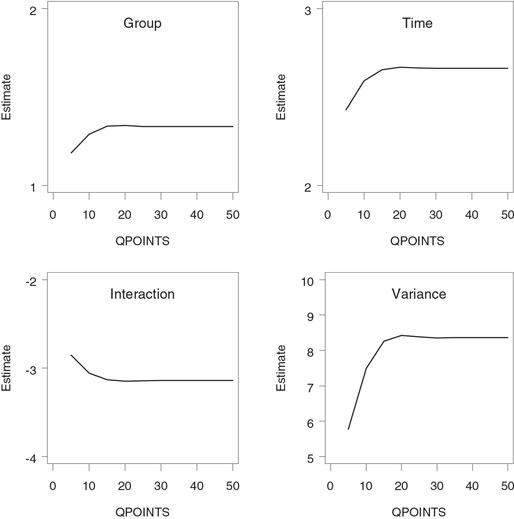
The PROC NLMIXED code in Program 3.17 uses the default numerical integration algorithm to approximate the marginal likelihood function of the binary responses (see Section 5.10 for a detailed discussion of numerical integration algorithms implemented in PROC NLMIXED). This is a very popular algorithm known as Gauss-Hermite quadrature (Liu and Pierce, 1994). The performance of the Gauss-Hermite quadrature approximation depends on the number of quadrature points specified by the QPOINTS parameter in PROC NLMIXED (Agresti and Hartzel, 2000). Choosing a large value of QPOINTS increases the accuracy of the numerical integration algorithm. Figure 3.12 demonstrates the relationship between the four parameter estimates in the logistic random effects model for AST levels and the value of the QPOINTS parameter. Figure 3.12 reveals that the parameter estimates do not stabilize until QPOINTS=30. Using the Gauss-Hermite quadrature algorithm with the default value of QPOINTS (5 points) will likely result in biased parameter estimates. It is prudent to routinely choose large values of the QPOINTS parameter (e.g., 50) in PROC NLMIXED when fitting nonlinear random effects models.
Random Effects Models for Ordinal Responses
The logistic random effects model for paired binary responses introduced in the previous subsection is easy to extend to the general case of ordinal variables. In order to show how to fit logistic random effects models for ordinal outcomes in PROC NLMIXED, it is convenient to adopt a slightly different specification of the likelihood function. As was mentioned above, the PROC NLMIXED code in Program 3.17 is fairly transparent and easy to follow. For example, it is clear from Program 3.17 that the P variable (probability of an abnormal AST result) is modeled as a function of four fixed effects and one normally distributed random effect with the logit link.
A less transparent but more flexible approach to modeling correlated categorical responses in PROC NLMIXED involves a direct specification of the conditional likelihood of responses given random subject effects. To illustrate, consider again the ulcerative colitis trial example with paired binary outcomes. Program 3.18 uses PROC NLMIXED to fit a logistic model with random subject effects to the data by maximizing the marginal likelihood function. However, unlike Program 3.17, this program does not explicitly indicate that the OUTCOME variable follows a binary distribution with the success probability P but rather tells SAS to work with the user-specified log-likelihood function. Since the specified log-likelihood function is a log-likelihood function for binary observations, the resulting PROC NLMIXED code is equivalent to the PROC NLMIXED code shown in Program 3.17 and produces identical output.
The advantage of the outlined alternative specification of the likelihood function is that it can be used to pass any likelihood function to PROC NLMIXED, including a likelihood function of observations on an ordinal scale. Consider the QTc interval prolongation example involving a comparison of QTc values
Figure 3.12 Effect of quadrature approximation on parameter estimates in a logistic random effects model
Program 3.18 Analysis of AST changes in the ulcerative colitis trial using a logistic random effects model
proc nlmixed data=ast2 qpoints=50;
parms intercept=-2.2 group=0.8 time=0.3 interaction=-1.8 sigmasq=1;
logit=intercept+group*gr+time*tm+interaction*int+se;
p0=1/(1+exp(logit));
p1=exp(logit)/(1+exp(logit));
if outcome=0 then logp=log(p0);
if outcome=1 then logp=log(p1);
model outcome~general(logp);
random se~normal(0,sigmasq) subject=subject;
run;
classified as normal, borderline and prolonged between two treatment groups (see Table 3.3). Program 3.19 fits a proportional odds model with random subject effects to the 3 × 3 shift tables in the placebo and experimental drug groups (with the initial values of the six parameters taken from Output 3.16). This model is similar to the GEE proportional odds model introduced in Section 3.3.1 (see Program 3.16) in that they both have two components (one for assessing the treatment effect on prolonged QTc intervals and the other for examining the treatment effect on both borderline and prolonged QTc intervals). However, the GEE and random effects models differ in the way they
Program 3.19 Analysis of QTc interval changes using a logistic random effects model
data qtcprol1;
set qtcprol;
do i=1 to count;
if therapy=″Placebo″ then gr=1; else gr=0;
subject=10000*gr+1000*baseline+100*endpoint+i;
outcome=baseline; tm=0; int=tm*gr; output;
outcome=endpoint; tm=1; int=tm*gr; output;
end;
proc nlmixed data=qtcprol1 qpoints=50;
ods select ParameterEstimates;
parms intercept1=-4.4 intercept2=-1.4 group=0.5 time=-0.2
interaction=-0.8 sigmasq=1;
logit1=intercept1+group*gr+time*tm+interaction*int+se;
logit2=intercept2+group*gr+time*tm+interaction*int+se;
p0=1/(1+exp(logit2));
p1=exp(logit2)/(1+exp(logit2))-exp(logit1)/(1+exp(logit1));
p2=exp(logit1)/(1+exp(logit1));
if outcome=0 then logp=log(p0);
if outcome=1 then logp=log(p1);
if outcome=2 then logp=log(p2);
model outcome~general(logp);
random se~normal(0,sigmasq) subject=subject;
run;
Output from Program 3.19
Parameter Estimates
| Parameter | Estimate | Standard Error |
DF | t Value | Pr > |t| | Alpha | Lower |
| intercept1 | -11.1595 | 2.4940 | 122 | -4.47 | <.0001 | 0.05 | -16.0966 |
| intercept2 | -5.0064 | 1.3380 | 122 | -3.74 | 0.0003 | 0.05 | -7.6552 |
| group | 0.3814 | 1.2437 | 122 | 0.31 | 0.7596 | 0.05 | -2.0806 |
| time | 2.1535 | 0.8254 | 122 | 2.61 | 0.0102 | 0.05 | 0.5196 |
| interaction | -1.6065 | 1.0830 | 122 | -1.48 | 0.1406 | 0.05 | -3.7505 |
| sigmasq | 17.4644 | 9.3402 | 122 | 1.87 | 0.0639 | 0.05 | -1.0255 |
Parameter Estimates
| Parameter | Upper | Gradient |
| intercept1 | -6.2223 | 0.000107 |
| intercept2 | -2.3576 | -0.00004 |
| group | 2.8434 | 0.000198 |
| time | 3.7874 | -0.00012 |
| interaction | 0.5375 | -0.00019 |
| sigmasq | 35.9543 | 0.000033 |
incorporate correlation between repeated measurements on the same subject. Since PROC GENMOD currently supports only the independent working covariance matrix for ordinal variables, Program 3.16 accounts for the correlations in repeated observations implicitly (through the empirical covariance matrix estimate). By contrast, the logistic model in Program 3.19 includes subject-specific random terms and thus explicitly accounts for the correlation between paired outcomes.
Output 3.19 displays estimates of the six model parameters produced by PROC NLMIXED. Note that the two logistic regression models fitted to the paired trinomial outcomes in the QTc prolongation example share all parameters with the exception of the intercept that becomes model-specific. INTERCEPT1 is the estimated intercept in the logistic model for prolonged QTc intervals and INTERCEPT2 is equal to the estimated intercept in the logistic model for borderline and prolonged QTc intervals.
We can see from Output 3.19 that the computed p-value for the TIME term is consistent in magnitude with the p-value produced by the GEE method (see Output 3.16). However, the p-value for the treatment effect, represented here by the INTERACTION term, is larger than that produced by the GEE method and is clearly non-significant. There is clearly not enough evidence to conclude that the two shift tables in the QTc interval prolongation example exhibit different change patterns.
3.3.3 Multinomial Likelihood Methods
This section reviews analysis methods for paired categorical variables based on direct models for cell probabilities in shift tables. The outlined modeling approach complements the methods described earlier in this chapter.
As was pointed out above, it is helpful to summarize paired categorical outcomes computed from quantitative diagnostic and safety measurements using shift tables. Once the shift tables have been constructed, the analysis of the categorical outcomes can be performed by comparing the patterns of change across the shift tables representing different treatment groups. Popular methods for the analysis of changes in shift tables described in Sections 3.3.1 and 3.3.2 rely primarily on comparing marginal distributions over time. For instance, the GEE approach focuses on regression parameters that characterize the marginal distribution of responses at each time point, whereas parameters describing the association across time points are treated as nuisance parameters. Although methods for performing simultaneous analyses of the regression and correlation parameters have been discussed in the literature (see, for example, Zhao and Prentice (1990)), they are rarely used in practice, partly due to their complexity.
By concentrating on the analysis of regression parameters, one essentially assumes that the marginal distribution of the endpoint measurements is a location shift of the baseline marginal distribution. This assumption may be fairly restrictive in a clinical trial setting. Tests of marginal homogeneity fail to capture clinically important trends when the location shift assumption is not met. To illustrate this fact, Dmitrienko (2003b) used an example from a two-arm Phase II clinical trial in which 205 patients underwent electrocardiographic (ECG) evaluations at baseline and endpoint. The ECG evaluations were all performed by the same cardiologist, who classified each ECG recording as normal or abnormal. Two 2 × 2 shift tables summarizing the results of these evaluations are presented in Table 3.4.
Table 3.4 The distribution of the overall ECG evaluations at baseline and endpoint in the two treatment groups
| Treatment group 1 | Treatment group 2 | |||||
| Endpoint | Endpoint | |||||
| Baseline | Normal | Abnormal | Baseline | Normal | Abnormal | |
| Normal | 83 | 1 | Normal | 80 | 7 | |
| Abnormal | 1 | 18 | Abnormal | 8 | 7 | |
It is easy to verify from Table 3.4 that the difference between the baseline and endpoint distributions of the overall ECG evaluations is very small. The likelihood of observing a normal overall ECG evaluation in Treatment group 1 is equal to 84/103=0.816 at baseline and 84/103=0.816 at endpoint. In Treatment group 2, this likelihood is equal to 87/102=0.853 at baseline and 88/102=0.863 at endpoint. As a result, using tests for homogeneity of marginal changes, one will likely conclude that the patterns of change are identical in the two treatment groups. For example, the following output was generated when the ECG data in Table 3.4 were analyzed using GEE and random effects models.
Analysis of changes in the overall ECG evaluations using a GEE model
Score Statistics For Type 3 GEE Analysis
| Source | DF | Chi- Square |
Pr > ChiSq |
| group | 1 | 0.80 | 0.3724 |
| time | 1 | 0.06 | 0.8042 |
| group*time | 1 | 0.06 | 0.8042 |
Analysis of changes in the overall ECG evaluations using a random effects model
Parameter Estimates
| Parameter | Estimate | Standard Error |
DF | t Value | Pr > |t| |
| intercept | -3.8464 | 0.7262 | 204 | -5.30 | <.0001 |
| group | 0.3767 | 0.8407 | 204 | 0.45 | 0.6546 |
| time | -0.1673 | 0.5790 | 204 | -0.29 | 0.7729 |
| interaction | 0.1673 | 0.8303 | 204 | 0.20 | 0.8405 |
| sigmasq | 10.1600 | 2.9416 | 204 | 3.45 | 0.0007 |
The output shown above lists the parameter estimates and associated test statistics produced by Programs 3.14 and 3.17. The treatment effect is represented here by the GROUP*TIME variable in the upper panel and the INTERACTION variable in the lower panel. The test statistics corresponding to these variables are very small, which means that the GEE and random effects models failed to detect the difference between the two shift tables. However, even a quick look at the data summarized in Table 3.4 reveals that the change patterns in the two shift tables are quite different. We can see from Table 3.4 that only one patient experienced worsening and only one patient experienced spontaneous improvement in Treatment group 1. In contrast, seven patients experienced worsening and eight patients experienced improvement in Treatment group 2. This finding may translate into a safety concern because the identified groups of improved and worsened patients most likely represent two different patient populations and do not cancel each other out. The observed difference in change patterns warrants additional analyses because it may imply that the drug administered to patients in Treatment group 2 causes harmful side effects. Similar examples can be found in Lindsey and Lambert (1998).
Inferences based on the regression parameters in GEE and random effects models fail to detect the treatment difference in Table 3.4 because the analysis of marginal changes is equivalent to the analysis of the off-diagonal cells and ignores the information in the main-diagonal cells. To improve the power of inferences based on marginal shifts, one needs to account for treatment-induced changes in both diagonal and off-diagonal cells. This can be accomplished by joint modeling of all cell probabilities in shift tables, rather than modeling the margins. A simple joint modeling method is based on grouping response vectors in 2 × 2 and more general shift tables into clinically meaningful categories and specifying a multinomial probability model for the defined response profiles. This approach was discussed by Dmitrienko (2003b) and is conceptually related to the modeling framework proposed by McCullagh (1978) and transition models described by Bonney (1987) and others.
To introduce the multinomial likelihood approach, suppose that a binary variable is measured at baseline and endpoint in a clinical trial with m treatment groups. The binary outcomes are coded as 0 and 1 and are summarized in m shift tables. Let Xi and Yi be selected at random from the marginal distribution of the rows and columns of the ith shift table. Since the response variable is binary and is measured at two time points, the response vector (Xi, Yi) assumes four values: (0,0), (0,1), (1,0) and (1,1). The paired observations with Xi = Yi and Xi = Yi are commonly termed concordant and discordant pairs, respectively.
The response vectors can be grouped in a variety of ways depending on the objective of the analysis. For example, one can consider the following partitioning scheme based on three categories in the ith treatment group:
Note that the concordant pairs are pooled together in this partitioning scheme to produce the category in the ith group because these cells do not contain information about treatment-induced changes. Next, consider the following model for this partitioning scheme:
where αi and βi are model parameters. It is instructive to compare this trinomial model to model (3.1) with a logit link function. Assuming two treatment groups, the group-by-time interaction in model (3.1) on the logit scale equals the difference in the β parameters in model (3.5). This means that by comparing the β parameters across the shift tables, one can draw conclusions about the homogeneity of marginal changes. Unlike model (3.1), the trinomial model includes the α parameters that summarize the relative weight of discordant pairs compared to concordant pairs (known as the discordance rate) in each shift table. A comparison of the α parameters helps detect treatment-induced changes in the diagonal cells.
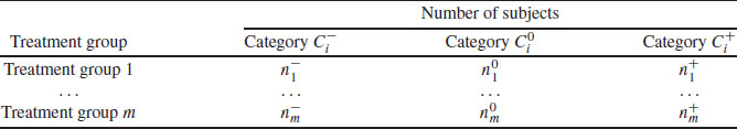
The introduced model for paired binary data can be extended to more general scenarios involving ordinal responses (Dmitrienko, 2003b). This section will concentrate on the analysis of the simple binary case. Let ni be the number of subjects in ith group and denote the numbers of subjects in Categories , and by , , respectively. Change patterns can be compared across the m treatment groups by testing the homogeneity of marginal changes (β1 = … = βm) and the equality of discordance rates (α1 = … = αm). Dmitrienko (2003b) showed that the likelihood-ratio test of this hypothesis is equivalent to the likelihood-ratio test for association in the m × 3 contingency table shown in Table 3.5.
Table 3.5 Contingency table used in comparing change patterns across m treatment groups
The likelihood-ratio test for association in Table 3.5 is easy to implement in PROC FREQ, which supports both asymptotic and exact versions of this test. Program 3.20 fits the trinomial model (3.5) to the paired binary data in Table 3.4 and estimates the α and β parameters in the two groups (note that the normal outcomes in the ECGEVAL data set are coded as 0 and abnormal outcomes are coded as 1). The program also computes p-values produced by the asymptotic and exact likelihood-ratio tests for the equality of change patterns in Treatment group 1 and Treatment group 2.
Program 3.20 Trinomial model for the changes in the overall ECG evaluations from baseline to endpoint
data ecgeval;
input therapy $ baseline endpoint count @@;
datalines;
| DrugA | 0 | 0 | 83 | DrugA | 1 | 0 | 1 | DrugA | 0 | 1 | 1 | DrugA | 1 | 1 | 18 |
| DrugB | 0 | 0 | 80 | DrugB | 1 | 0 | 8 | DrugB | 0 | 1 | 7 | DrugB | 1 | 1 | 7 |
;
data transform;
set ecgeval;
if baseline+endpoint^=1 then change=″Same″;
if baseline=0 and endpoint=1 then change=″Up″;
if baseline=1 and endpoint=0 then change=″Down″;
proc sort data=transform;
by therapy change;
proc means data=transform noprint;
by therapy change;
var count;
output out=sum sum=sum;
data estimate;
set sum;
by therapy;
retain nminus nzero nplus;
if change=″Same″ then nzero=sum;
if change=″Up″ then nplus=sum;
if change=″Down″ then nminus=sum;
alpha=(nminus+nplus)/(nminus+nzero+nplus);
if nminus+nplus>0 then beta=nplus/(nminus+nplus); else beta=1;
if last.therapy=1;
keep therapy beta alpha;
proc print data=estimate noobs;
proc freq data=sum;
ods select LRChiSq;
table therapy*change;
exact lrchi;
weight sum;
run;
Output from Program 3.20
| therapy | alpha | beta |
| DrugA | 0.01942 | 0.50000 |
| DrugB | 0.14706 | 0.46667 |
Likelihood Ratio Chi-Square Test
| Chi-Square | 12.2983 | |
| DF | 2 | |
| Asymptotic | Pr > ChiSq | 0.0021 |
| Exact | Pr >= ChiSq | 0.0057 |
Output 3.20 lists the estimated α and β parameters in the two treatment groups accompanied by the asymptotic and exact likelihood ratio p-values. We see that there is little separation between the β parameters, which indicates that the magnitudes of marginal changes are in close agreement in the two treatment groups. However, the discordance rate in Treatment group 1 is much smaller than that in Treatment group 2 (α1 = 0.019 and α2 = 0.147, respectively). The asymptotic test statistic for the homogeneity of treatment-induced changes is equal to 12.2983 with 2 degrees of freedom and is highly significant (p = 0.0021). The exact likelihood-ratio p-value, which is more reliable in this situation, is also highly significant (p = 0.0057). Both the asymptotic and exact tests clearly indicate that different patterns of change in the overall ECG evaluation are observed in the two treatment groups.
3.3.4 Summary
This section reviewed methods for the analysis of repeated categorical outcomes. Although the focus of the section was on responses derived from quantitative safety and diagnostic measures, the described methods can be successfully used in any statistical problem involving repeated categorical responses, such as in longitudinal efficacy analyses.
The two most popular approaches to the analysis of categorical data in a longitudinal setting are based on generalized estimating equations and random effects models. We demonstrated in this section how to perform GEE inferences using PROC GENMOD both in the case of binary and ordinal responses. GEE methods produce consistent estimates of the regression parameters that are robust with respect to the working covariance matrix. Although regression estimates become less efficient if the selected correlation structure substantially differs from the true correlation structure, their consistency is not affected by the wrong choice of the working covariance matrix. GEE methods are attractive in clinical applications because they allow the statistician to consistently estimate the model parameters when no prior information is available to aid in the selection of a correlation structure.
GEE models are commonly referred to as population-averaged models because they describe an average of responses in the underlying population at each particular time point. Population-averaged inferences need to be carefully interpreted in a clinical trial setting because they do not adequately account for the between-subject heterogeneity. It is well known that samples of patients recruited in clinical trials are not randomly selected from a larger population of patients. When the resulting sample is highly heterogeneous, response profiles produced by GEE methods may not correspond to any possible patient and therefore can sometimes be misleading.
The other widely used analysis method relies on random effects models for repeated categorical measurements. The random effects models include a subject-specific random term and thus account for the heterogeneity of subjects’ response profiles. Parameter estimation in the random effects models is typically performed based on marginal likelihood and requires a substantial amount of numerical integration. PROC NLMIXED helps the statistician solve the computational problem and make inferences in a wide class of nonlinear random effects models.
Finally, this section discussed analysis of paired categorical variables based on direct models for cell probabilities in shift tables. This modeling approach complements the GEE and logistic random effects methods in the analysis of shift tables with identical or virtually identical marginal distributions.