
4.3 Stochastic Curtailment Tests
We have pointed out repeatedly throughout the chapter that pivotal clinical trials are routinely monitored to find early evidence of beneficial or harmful effects. Section 4.2 introduced an approach to the design and analysis of group sequential trials based on repeated significance testing. This section looks at sequential testing procedures used in a slightly different context. Specifically, it reviews recent advances in the area of stochastic curtailment with emphasis on procedures for futility monitoring.
To help understand the difference between repeated significance and stochastic curtailment tests, recall that repeated significance testing is centered around the notion of error spending. The chosen error spending strategy determines the characteristics of a sequential test (e.g., the shape of stopping boundaries) and ultimately drives the decision-making process. In the stochastic curtailment framework, decision making is tied directly to the final trial outcome. A decision to continue the trial or curtail sampling at each interim look is based on the likelihood of observing a positive or negative treatment effect if the trial were to continue to the planned end. Another important distinction is that stochastic curtailment methods are aimed toward predictive inferences, whereas repeated significance tests focus on currently available data.
Stochastic curtailment procedures (especially futility rules) are often employed in clinical trials with a fixed-sample design without an explicit adjustment for repeated statistical analyses. It is not unusual to see a stochastic curtailment test used in a post hoc manner; for example, a futility rule may be adopted after the first patient visit.
This section reviews three popular types of stochastic curtailment tests with emphasis on constructing futility rules. Section 4.3.1 introduces frequentist methods commonly referred to as conditional power methods. We will discuss the conditional power test developed by Lan, Simon and Halperin (1982) and Halperin et al. (1982) as well as its adaptive versions proposed by Pepe and Anderson (1992) and Betensky (1997). Next, Sections 4.3.2 and 4.3.3 cover mixed Bayesian-frequentist and fully Bayesian methods considered, among others, by Herson (1979), Spiegelhalter, Freedman, and Blackburn (1986), Geisser (1992), Geisser and Johnson (1994), Johns and Anderson (1999) and Dmitrienko and Wang (2006).
The following two examples will be used to illustrate the methods for constructing futility rules reviewed in this section.
EXAMPLE: Generalized Anxiety Disorder Trial with a Continuous Endpoint
A small proof-of-concept trial in patients with generalized anxiety disorder will serve as an example of a trial with a continuous outcome variable. In this trial, patients were randomly assigned to receive an experimental drug or a placebo for 6 weeks. The efficacy profile of the drug was evaluated using the mean change from baseline in the Hamilton Anxiety Rating Scale (HAMA) total score. The total sample size was 82 patients (41 patients were to be enrolled in each of the two treatment arms). This sample size provides approximately 80% power to detect a treatment difference of 4 in the mean HAMA total score change. The power calculation is based on a one-sided test with an α-level of 0.1 and assumes a standard deviation of 8.5.
The trial was not intended to be stopped early in order to declare efficacy; however, HAMA total score data were monitored in this trial to detect early signs of futility or detrimental effects. Table 4.11 summarizes the results obtained at three interim looks. Note that the experimental drug improves the HAMA total score by decreasing it and thus negative changes in Table 4.11 indicate improvement.
Table 4.11 HAMA total score data in the generalized anxiety disorder trial
| Experimental group | Placebo group | ||||
| Interim analysis |
n | Mean HAMA change (SD) |
n | Mean HAMA change (SD) |
|
| 1 | 10 | –9.2 (7.3) | 11 | –8.4 (6.4) | |
| 2 | 20 | –9.4 (6.7) | 20 | –8.1 (6.9) | |
| 3 | 31 | -8.9 (7.4) | 30 | -9.1 (7.7) | |
EXAMPLE: Severe Sepsis Trial with a Binary Endpoint
Consider a two-arm clinical trial in patients with severe sepsis conducted to compare the effect of an experimental drug on 28-day all-cause mortality to that of a placebo. The trial design included a futility monitoring component based on monthly analyses of the treatment effect on survival. The total sample size of 424 patients was computed to achieve 80% power of detecting a 9% absolute improvement in the 28-day survival rate at a one-sided significance level of 0.1. This calculation was based on the assumption that the placebo survival rate is 70%.
The trial was discontinued after approximately 75% of the projected number of patients had completed the 28-day study period because the experimental drug was deemed unlikely to demonstrate superiority to the placebo at the scheduled termination point. Table 4.12 provides a summary of the mortality data at six interim analyses conducted prior to the trial’s termination.
In both of these clinical trial examples we are interested in setting up a futility rule to help assess the likelihood of a positive trial outcome given the results observed at each of the interim looks.
Table 4.12 Survival data in the severe sepsis trial
| Experimental group | Placebo group | ||||||
| Interim analysis |
Total | Alive | Survival | Total | Alive | Survival | |
| 1 | 55 | 33 | 60.0% | 45 | 29 | 64.4% | |
| 2 | 79 | 51 | 64.6% | 74 | 29 | 66.2% | |
| 3 | 101 | 65 | 64.4% | 95 | 62 | 65.3% | |
| 4 | 117 | 75 | 64.1% | 115 | 77 | 67.0% | |
| 5 | 136 | 88 | 64.7% | 134 | 88 | 65.7% | |
| 6 | 155 | 99 | 63.9% | 151 | 99 | 65.6% | |
4.3.1 Futility Rules Based on Conditional Power Lan-Simon-Halperin Conditional Power Test
To introduce the Lan-Simon-Halperin test, consider a two-arm clinical trial with N patients per treatment group and assume that we are planning to take an interim look at the data after n patients have completed the trial in each treatment group. Let Zn be the test statistic computed at the interim look; i.e.,
Zn=^δnˆσ√2/n,
where ˆδn
ZN=^δNˆσ√2/N.
Finally, δ and σ will denote the true treatment difference and common standard deviation of the response variable in the two treatment groups. This formulation of the problem can be used with both continuous and binary endpoints.
The conditional power test proposed by Lan, Simon and Halperin (1982) is based on an intuitively appealing idea of predicting the distribution of the final outcome given the data already observed in the trial. If the interim prediction indicates that the trial outcome is unlikely to be positive, ethical and financial considerations will suggest an early termination the trial. Mathematically, the decision rule can be expressed in terms of the probability of a statistically significant outcome—i.e., ZN > z1—α, conditional on the interim test statistic Zn. This conditional probability is denoted by Pn (δ) and is termed conditional power. The trial is stopped as soon as the conditional power falls below a prespecified value 1 – γ, where γ is known as the futility index (Ware, Muller and Braunwald, 1985). Smaller values of γ are associated with a higher likelihood of early stopping and, most commonly, γ is set to a value between 0.8 and 1.
It was shown by Lan, Simon and Halperin (1982) that the outlined futility rule has a simple structure and is easy to apply in clinical trials with continuous or binary outcome variables (see Jennison and Turnbull (1990) for more details). Suppose that the test statistics Zn and ZN are jointly normally distributed and δ and σ are known. In this case, the conditional distribution of ZN given Zn is normal with
mean=√nNZn+δ(N-n)σ√2N and variance =N−nN.
Therefore the conditional power function Pn (δ) is given by
Pn(δ)=Φ(σ√nZn+(N−n)δ/√2−σ√Nz1−ασ√N−n).
As before, z1—α denotes the 100(1 — α)th percentile of the standard normal distribution and Φ(x) is the cumulative probability function of the standard normal distribution.
A stopping rule can now be formulated in terms of the computed conditional power:
Terminate the trial due to lack of efficacy the first time Pn (δ) < 1 – γ,
or in terms of the observed test statistic Zn :
Terminate the trial due to lack of efficacy the first time Zn < ln,
where the adjusted critical value ln is given by
ln=√Nnz1−α+√N−nnz1−γ−δ(Ν-n)σ√2n.
It is clear that the introduced futility rule is heavily influenced by the assumed value of the treatment difference δ. The clinical trial will be stopped sooner if δ is small and vice versa. Lan, Simon and Halperin (1982) and Halperin et al. (1982) considered stochastic curtailment tests in which the conditional power function was evaluated at the value of δ corresponding to the alternative hypothesis. With this choice of δ, conditional power is computed assuming that future data are generated from the alternative hypothesis.
It is interesting to note that the resulting conditional power procedure is closely related to group sequential testing procedures discussed in Section 4.2. Jennison and Turnbull (1990) pointed out that a special case of the Lan-Simon-Halperin test is a continuous-time equivalent of the O’Brien-Fleming group sequential test. Davis and Hardy (1990) showed that the stopping boundary of the Lan-Simon-Halperin test for efficacy monitoring with γ = 0.5 is virtually equivalent to the stopping boundary of the O’Brien-Fleming test. Likewise, if one constructs the O’Brien-Fleming boundary for testing lack of treatment benefit, it will be very close to the stopping boundary of the Lan-Simon-Halperin test with γ = 0.5. Note, however, that the futility index γ is typically set at the 0.8 or higher level in clinical trials. Thus, the O’Brien-Fleming test for futility (and other repeated significance procedures) is more likely to trigger an early stopping due to lack of efficacy compared to the Lan-Simon-Halperin test.
%CondPowerLSH Macro
Program 4.17 applies the Lan-Simon-Halperin conditional power test to the analysis of the severe sepsis trial. The program computes the z statistics for the treatment effect at each of the 6 interim analyses and then calls the %CondPowerLSH macro provided in the Appendix to estimate the conditional probability of a positive trial outcome under the alternative hypothesis. The %CondPowerLSH macro has the following arguments:
• DATA is the name of the input data set with one record per interim look. The data set must include the following variables:
– N is the number of patients per group included in the analysis data set at the current interim look. If the sample sizes are unequal in the two treatment groups, set N to the average of the two sample sizes.
– TESTSTAT is the test statistic computed at the current interim look.
• EFFSIZE is the hypothesized effect size (i.e., the treatment effect divided by the standard deviation).
• ALPHA is the one-sided Type I error probability of the significance test carried out at the end of the trial.
• GAMMA is the futility index.
• NN is the projected number of patients per treatment group.
• PROB is the name of the data set containing the computed conditional power at each interim look. This data set is generated by the macro and includes the following variables:
– ANALYSIS is the analysis number.
– FRACTION is the fraction of the total sample size.
– TESTSTAT is the test statistic from the input data set.
– CONDPOWER is the computed conditional power.
• BOUNDARY is the name of the data set that contains the stopping boundary of the conditional power test. This data set is generated by the macro and includes the following variables:
– FRACTION is the fraction of the total sample size.
– STOPBOUNDARY is the stopping boundary on the test statistic scale.
In order to invoke the %CondPowerLSH macro, we need to specify the effect size under the alternative hypothesis. Assuming 28-day survival rates of 0.7 and 0.79 in the two treatment groups, the treatment difference δ is 0.09 and the pooled standard deviation σ is
√0.745(1−0.745)=0.436,
where 0.745 is the average survival rate in the two treatment groups. Therefore, the effect size is equal to
δ/σ = 0.09/0.436 = 0.2065
and we will let EFFSIZE=0.2065. From the severe sepsis trial example, the one-sided significance level ALPHA is 0.1 and the projected sample size per group NN is 212. Lastly, we will set the futility index GAMMA to 0.8 to avoid very early stopping. With this choice of the futility index, the trial will be stopped as soon as the conditional probability of detecting a statistically significant difference at the planned end falls below 0.2.
Program 4.17 Lan-Simon-Halperin conditional power test in the analysis of the severe sepsis trial
data sevsep;
input ExpN ExpAlive PlacN PlacAlive;
datalines;
| 55 | 33 | 45 | 29 |
| 79 | 51 | 74 | 49 |
| 101 | 65 | 95 | 62 |
| 117 | 75 | 115 | 77 |
| 136 | 88 | 134 | 88 |
| 155 | 99 | 151 | 99 |
| ; | |||
data test;
set sevsep;
diff=ExpAlive/ExpN-PlacAlive/PlacN;
ave=(ExpAlive/ExpN+PlacAlive/PlacN)/2;
n=(ExpN+PlacN)/2;
teststat=diff/sqrt(2*ave*(1-ave)/n);
keep n teststat;
%CondPowerLSH(data=test,effsize=0.2065,alpha=0.1,gamma=0.8,nn=212,
prob=p,boundary=boundary);
proc print data=p noobs label;
data test;
set test;
group=1;
fraction=n/212;
StopBoundary=teststat;
data boundary;
set boundary;
group=2;
data plot;
set test boundary;
axis1 minor=none label=(angle=90 “Test statistic”) order=(-3 to 1 by 1);
axis2 minor=none label=(“Fraction of total sample size”)
order=(0 to 1 by 0.2);
symbol1 i=none v=dot color=black;
symbol2 i=join v=none color=black line=1;
proc gplot data=plot;
plot StopBoundary*Fraction=group/frame nolegend
haxis=axis2 vaxis=axis1 vref=0 lvref=34;
run;
Output from Program 4.17
| Analysis | Fraction of total sample size |
Test statistic |
Conditional power |
| 1 | 0.24 | –0.4583 | 0.5548 |
| 2 | 0.36 | –0.2157 | 0.4739 |
| 3 | 0.46 | –0.1329 | 0.3776 |
| 4 | 0.55 | –0.4573 | 0.1644 |
| 5 | 0.64 | –0.1666 | 0.1433 |
| 6 | 0.72 | –0.3097 | 0.0354 |
Output 4.17 indicates that, despite a negative treatment difference at the first interim look, there is still a 55% chance that the trend will be reversed by the completion of the trial if the absolute treatment difference is truly equal to 9%. This probability is fairly high and suggests that the trial should be continued to the next interim analysis. However, we do not see any improvement in the conditional power over the next several looks. In fact, the conditional probability of a statistically significant outcome at the planned end of the trial decreases steadily over time and becomes exceedingly small by the last look. A close examination of the right-hand column in Output 4.17 reveals a notable drop in the conditional power approximately halfway into the trial (at the fourth interim look). Since the conditional power is below the prespecified 20% threshold, we conclude that the observed treatment difference is no longer consistent with the alternative hypothesis and the trial should have been terminated due to futility at the fourth interim analysis.
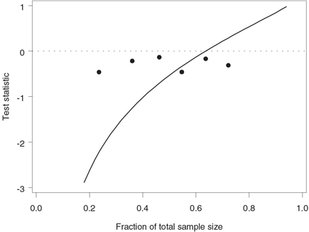
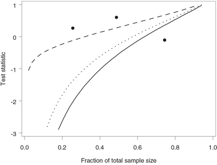
Figure 4.24 depicts the test statistics computed at the six interim analyses plotted along with the stopping boundary corresponding to the futility index of 0.8. The stopping boundary lies well below 0 at the time of the first look but catches up with the test statistics toward the midpoint of the trial. This confirms our conclusion that there is an early trend in favor of continuing the trial. Note that the stopping boundary crosses the dotted line drawn at z = 0 when n /N = 0.64, which implies that any negative treatment difference observed beyond this point would cause the trial to be stopped due to lack of treatment benefit.
Program 4.18 produces an alternative graphical representation of the Lan-Simon-Halperin futility boundary in the severe sepsis trial.Instead of focusing on the z statistics computed at each of the six interim looks, the program plots stopping boundaries expressed in terms of observed survival rates. The stopping boundary is computed by fixing the survival rate in the experimental group and finding the smallest placebo survival rate for which the conditional probability of a statistically significant difference at the scheduled end of the trial is less than 1 – γ = 0.2.
Figure 4.24 Stopping boundary of the Lan-Simon-Halperin test (—) and interim z statistics (•) in the severe sepsis trial example. The futility index γ is 0.8; the continuation region is above the stopping boundary.
Program 4.18 Alternative representation of the Lan-Simon-Halperin futility boundaries in the severe sepsis trial
proc iml;
expn={55, 79, 101, 117, 136, 155};
placn={45, 74, 95, 115, 134, 151};
lower=0.2;
upper=0.8;
nn=212;
alpha=0.1;
effsize=0.2065;
gamma=0.8;
boundary=j(1,3,.);
do analysis=1 to 6;
start=ceil(expn[analysis]*lower);
end=floor(expn[analysis]*upper);
temp=j(end-start+1,3,0);
do i=start to end;
p1=i/expn[analysis];
j=ceil(placn[analysis]*lower)-1;
prob=1;
do while(prob>1-gamma & j<=placn[analysis]);
j=j+1;
p2=j/placn[analysis];
ave=(p1+p2)/2;
n=(expn[analysis]+placn[analysis])/2;
teststat=(p1-p2)/sqrt(2*ave*(1-ave)/n);
prob=1-probnorm((sqrt(nn)*probit(1-alpha)-sqrt(n)*teststat
-(nn-n)*effsize/sqrt(2))/sqrt(nn-n));
end;
k=i-start+1;
temp[k,1]=p1;
temp[k,2]=p2;
temp[k,3]=analysis;
end;
boundary=boundary//temp;
end;
varnames={"p1" "p2" "analysis"};
create boundary from boundary[colname=varnames];
append from boundary;
quit;
data points;
p1=33/55; p2=29/45; analysis=7; output;
p1=51/79; p2=49/74; analysis=8; output;
p1=65/101; p2=62/95; analysis=9; output;
p1=75/117; p2=77/115; analysis=10; output;
p1=88/136; p2=88/134; analysis=11; output;
p1=99/155; p2=99/151; analysis=12; output;
data boundary;
set boundary points;
%macro BoundPlot(subset,analysis);
axis1 minor=none label=(angle=90 "Observed survival rate (Placebo)")
order=(0.5 to 0.8 by 0.1);
axis2 minor=none label=("Observed survival rate (Exp drug)")
order=(0.5 to 0.8 by 0.1);
symbol1 i=j v=none color=black line=1;
symbol2 i=none v=dot color=black;
data annotate;
xsys="1"; ysys="1"; hsys="4"; x=50; y=10; position="5";
size=1; text="Interim analysis &analysis"; function="label";
proc gplot data=boundary anno=annotate;
where ⊂
plot p2*p1=analysis/frame nolegend haxis=axis2 vaxis=axis1;
run;
quit;
%mend BoundPlot;
%BoundPlot(%str(analysis in (1,7)),1);
%BoundPlot(%str(analysis in (2,8)),2);
%BoundPlot(%str(analysis in (3,9)),3);
%BoundPlot(%str(analysis in (4,10)),4);
%BoundPlot(%str(analysis in (5,11)),5);
%BoundPlot(%str(analysis in (6,12)),6);
Figure 4.25 displays the Lan-Simon-Halperin stopping boundaries with the futility index γ = 0.8 on an event rate scale. Since the Lan-Simon-Halperin test depends on the data through the Zn statistic, the associated decision rule is driven mainly by the treatment difference and is not affected by the actual values of survival rates. As a consequence, the stopping boundaries in Figure 4.25 look like straight-line segments parallel to the identity line.
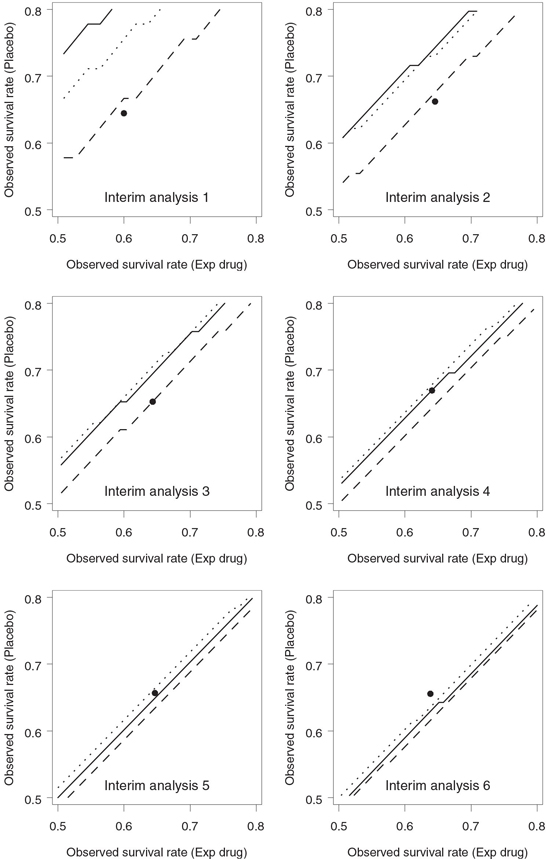
Stopping boundaries plotted on an event rate scale have a number of advantages that make them very appealing in a clinical trial setting. First, they facilitate the communication of interim findings to medical colleagues. Second, the stopping boundaries in Figure 4.25 help appreciate the effect of each additional death on the decision making process. Consider, for example, the fourth interim analysis. Figure 4.24 shows that the corresponding z statistic lies well below the stopping boundary and the survival rate in the experimental group is clearly too low to justify the continuation of the trial. However, Figure 4.25 demonstrates that the dot representing the observed survival rates sits right on the stopping boundary. Thus, instead of a clear-cut decision, we are likely dealing here with a borderline situation in which one additional death in the placebo group could easily change the conclusion. A simple sensitivity analysis proves that this is in fact the case. Assuming 75 survivors in the experimental group, one can check that an additional death in the placebo group would cause the dot at the fourth interim look to move into the continuation region.
Figure 4.25 Stopping boundary of the Lan-Simon-Halperin test (—) and interim survival rates (•) in the severe sepsis trial example. The futility index γ is 0.8; the continuation region is below the stopping boundary.

The last remark in this subsection is concerned with the effect of futility monitoring on the power of a clinical trial. Due to the possibility of early stopping in favor of the null hypothesis, any futility monitoring strategy results in power loss, and it is important to assess the amount of Type II error rate inflation. Toward this end, Lan, Simon and Halperin (1982) derived an exact lower bound for the power of their test. They showed that the power under the alternative hypothesis cannot be less than 1 – β/γ. For example, the power of the severe sepsis trial with β = 0.2 employing the Lan-Simon-Halperin futility rule will always exceed 77.8% if γ = 0.9 and 71.4% if γ = 0.7, regardless of the number of interim analyses.
Although it is uncommon to do so, we can theoretically use the obtained lower bound to recalculate the sample size and bring the power back to the desired level. After the sample size has been adjusted, we can apply the Lan-Simon-Halperin futility rule an arbitrary number of times without compromising the trial’s operating characteristics. For instance, in order to preserve the Type II error rate at the 0.2 level, the power of the severe sepsis trial needs to be set to 1 – βγ, which is equal to 82% if γ = 0.9 and 86% if γ = 0.7. To see how this affects the trial’s size, recall that the original fixed-sample design with a one-sided α-level of 0.1 and 80% power requires 424 patients. To achieve 82% power, the number of patients will have to be increased to 454 (7% increase). Similarly, 524 patients (24% increase) will need to be enrolled in the trial to protect the Type II error probability if γ = 0.7.
One should remember that the exact lower bound for the overall power is rather conservative and is achieved only in clinical trials with a very large number of interim looks (especially if γ is less than 0.7). If recomputing the sample size appears feasible, one can also consider an approximation to the power function of the Lan-Simon-Halperin test developed by Davis and Hardy (1990); see also Betensky (1997).
Adaptive Conditional Power Tests
An important feature of the Lan-Simon-Halperin test introduced in the previous subsection is the assumption that future observations are generated from the alternative hypothesis. It has been noted in the literature that this assumption may lead to spurious results and, as a consequence, the corresponding conditional power test does not always serve as a reliable stopping criterion. For example, Pepe and Anderson (1992) reviewed the performance of the Lan-Simon-Halperin test under a scenario when interim data do not support the alternative hypothesis. They showed that the Lan-Simon-Halperin test tends to produce an overly optimistic probability of a positive trial outcome when the observed treatment effect is substantially different from the hypothesized one.
To illustrate this phenomenon, consider the severe sepsis trial example. The trial was designed under the assumption that the experimental drug provides a 9% absolute improvement in the 28-day survival rate. The interim data displayed in Table 4.12 clearly contradict the alternative hypothesis: the treatment difference remains negative at all six interim looks. In this situation it is natural to ask whether adjusting the original assumptions to account for the emerging pattern will have an effect on the decision-making process. Program 4.19 performs conditional power calculations under assumptions that are more consistent with the interim data than the alternative hypothesis; specifically, the effect size for the future data is set to 0.1 and 0.
Program 4.19 Lan-Simon-Halperin conditional power test in the analysis of the severe sepsis trial under less optimistic assumptions about the magnitude of the treatment effect
%CondPowerLSH(data=test,effsize=0.1,alpha=0.1,gamma=0.8,nn=212,
prob=p,boundary=boundary);
title "Effect size is 0.1";
proc print data=p noobs label;
%CondPowerLSH(data=test,effsize=0,alpha=0.1,gamma=0.8,nn=212,
prob=p,boundary=boundary);
title "Effect size is 0";
proc print data=p noobs label;
run;
Output from Program 4.19
| Effect size is 0.1 | ||||||
| Analysis | Fraction of total sample size |
Test statistic |
Conditional power |
|||
| 1 | 0.24 | -0.4583 | 0.2059 | |||
| 2 | 0.36 | -0.2157 | 0.1731 | |||
| 3 | 0.46 | -0.1329 | 0.1322 | |||
| 4 | 0.55 | -0.4573 | 0.0432 | |||
| 5 | 0.64 | -0.1666 | 0.0421 | |||
| 6 | 0.72 | -0.3097 | 0.0085 | |||
| Effect size is 0 | ||||||
| Analysis | Fraction of total sample size |
Test statistic |
Conditional power |
|||
| 1 | 0.24 | -0.4583 | 0.0427 | |||
| 2 | 0.36 | -0.2157 | 0.0388 | |||
| 3 | 0.46 | -0.1329 | 0.0307 | |||
| 4 | 0.55 | -0.4573 | 0.0080 | |||
| 5 | 0.64 | -0.1666 | 0.0095 | |||
| 6 | 0.72 | -0.3097 | 0.0017 | |||
It is instructive to compare Output 4.19 with Output 4.17, in which the conditional power was computed under the alternative hypothesis and thus the effect size for the future data was set to 0.2065. The conditional power values in Output 4.19 are consistently lower than those in Output 4.17 with the conditional power estimates in the bottom half being extremely small right from the first futility analysis. This observation has a simple explanation. Since the true effect size for the future observations is assumed to be smaller in magnitude, there is a lower chance that the negative treatment difference will get reversed by the end of the trial and thus the conditional power of a positive trial outcome will also be lower. We can see from Output 4.19 that making an overly optimistic assumption about the size of the treatment effect delays the decision to terminate the trial and can potentially cause more patients to be exposed to an ineffective therapy. For this reason, in the absence of strong a priori evidence it may be inappropriate to use the alternative hypothesis for generating future data in conditional power calculations.
Since failure to account for emerging trends may undermine the utility of the simple conditional power method, Lan and Wittes (1988) proposed to evaluate the conditional power function at a data-driven value. Pepe and Anderson (1992) studied a conditional power test using the value of the treatment difference that is slightly more optimistic than the interim maximum likelihood estimate. This and similar adaptive approaches achieve greater efficiency than the simple conditional power method by “letting the data speak for themselves.”
Using the Pepe-Anderson test as a starting point, Betensky (1997) introduced a family of adaptive conditional power tests in which the fixed value of δ is replaced in the decision rule with ˆδn+cSE(ˆδn)
Using our notation and assuming σ is known, it is easy to check that
^δn=σ√2/nZn
and
SE(^δn)=σ√2/n.
Therefore, the resulting Pepe-Anderson-Betensky decision rule is based on the conditional probability
Pn=Φ(√nZn+(N−n)(Zn+c)/√n−√Nz1−α√N−n),
and the trial is stopped the first time Pn is less than 1 – γ. Note that this futility rule no longer depends on the standard deviation of the outcome variable (σ).
Equivalently, the Pepe-Anderson-Betensky rule can be formulated in terms of the test statistic Zn. Specifically, the trial is terminated as soon as the test statistic drops below the adjusted critical value defined as follows:
ln=√nNz1−α+√n(N−n)N2z1−γ−c(N−n)N.
%CondPowerPAB Macro
Program 4.20 uses the Pepe-Anderson-Betensky test with c = 1 and c = 2.326 as the stopping criterion in the severe sepsis trial. The Pepe-Anderson-Betensky test is implemented in the %CondPowerPAB macro given in the Appendix. To call the %CondPowerPAB macro, we need to provide information similar to that required by the %CondPowerLSH macro:
• DATA is the name of the input data set with one record per interim look. The data set must include the N and TESTSTAT variables defined as in the %CondPowerLSH macro.
• ALPHA is the one-sided Type I error probability of the significance test carried out at the end of the trial.
• GAMMA is the futility index.
• C is the parameter determining the shape of the stopping boundary. Pepe and Anderson (1992) set C to 1 and Betensky (1997) recommended to set C to 2.326.
• NN is the projected number of patients per treatment group.
• PROB is the name of the data set containing the computed conditional power. This data set is generated by the macro and includes the ANALYSIS, FRACTION, TESTSTAT and CONDPOWER variables defined as in the %CondPowerLSH macro.
• BOUNDARY is the name of the data set that contains the stopping boundary of the conditional power test. This data set is generated by the macro and includes the FRACTION and STOPBOUNDARY variables defined as in the %CondPowerLSH macro.
The main difference between the %CondPowerLSH and %CondPowerPAB macros is that in order to generate future data the latter macro relies on a sample estimate of the effect size and thus it no longer requires the specification of the effect size under the alternative hypothesis.
Program 4.20 Pepe-Anderson-Betensky conditional power test in the analysis of the severe sepsis trial
%CondPowerPAB(data=test,alpha=0.1,gamma=0.8,c=1,nn=212,
prob=p,boundary=boundary1);
title "Pepe-Anderson-Betensky test with c=1";
proc print data=p noobs label;
%CondPowerPAB(data=test,alpha=0.1,gamma=0.8,c=2.326,nn=212,
prob=p,boundary=boundary2);
%CondPowerLSH(data=test,effsize=0.2065,alpha=0.1,gamma=0.8,nn=212,
prob=p,boundary=boundary3);
title "Pepe-Anderson-Betensky test with c=2.326";
proc print data=p noobs label;
run;
data test;
set test;
group=1;
fraction=n/212;
StopBoundary=teststat;
data boundary1;
set boundary1;
group=2;
data boundary2;
set boundary2;
group=3;
data boundary3;
set boundary3;
group=4;
data plot;
set test boundary1 boundary2 boundary3;
axis1 minor=none label=(angle=90 "Test statistic") order=(-3 to 1 by 1);
axis2 minor=none label=("Fraction of total sample size")
order=(0 to 1 by 0.2);
symbol1 i=none v=dot color=black;
symbol2 i=join v=none color=black line=20;
symbol3 i=join v=none color=black line=34;
symbol4 i=join v=none color=black line=1;
proc gplot data=plot;
plot StopBoundary*Fraction=group/frame nolegend
haxis=axis2 vaxis=axis1;
run;
quit;
Output from Program 4.20
| Pepe-Anderson-Betensky test with c=1 | ||||||
| Analysis | Fraction of total sample size |
Test statistic |
Conditional power |
|||
| 1 | 0.24 | -0.4583 | 0.2279 | |||
| 2 | 0.36 | -0.2157 | 0.2354 | |||
| 3 | 0.46 | -0.1329 | 0.1747 | |||
| 4 | 0.55 | -0.4573 | 0.0278 | |||
| 5 | 0.64 | -0.1666 | 0.0429 | |||
| 6 | 0.72 | -0.3097 | 0.0062 | |||
| Pepe-Anderson-Betensky test with c=2.326 | ||||||
| Analysis | Fraction of total sample size |
Test statistic |
Conditional power |
|||
| 1 | 0.24 | -0.4583 | 0.9496 | |||
| 2 | 0.36 | -0.2157 | 0.8516 | |||
| 3 | 0.46 | -0.1329 | 0.6895 | |||
| 4 | 0.55 | -0.4573 | 0.2397 | |||
| 5 | 0.64 | -0.1666 | 0.2370 | |||
| 6 | 0.72 | -0.3097 | 0.0469 | |||
Output 4.20 displays the conditional power estimates at the six interim looks produced by the Pepe-Anderson-Betensky test under two scenarios. Under the first scenario (c = 1), this test is more likely to lead to early termination than the Lan-Simon-Halperin test. The conditional power is very close to the 20% threshold at the very first interim analysis, suggesting that the alternative hypothesis is unlikely to be true. The conditional power falls below the threshold and the test rejects the alternative at the third analysis. The early rejection of the alternative hypothesis is consistent with the observation that the experimental drug is unlikely to improve survival and might even have a detrimental effect on patients’ health.
In contrast, the Pepe-Anderson-Betensky test with c = 2.326 relies on a stopping boundary that virtually excludes the possibility of an early termination. The initial conditional power values are well above 50%. Although the conditional power decreases steadily, it remains above the 20% threshold at the fourth and fifth looks. The stopping criterion is not met until the last analysis.
Figure 4.26 depicts the Pepe-Anderson-Betensky stopping boundaries corresponding to c = 1 and c = 2.326 along with the stopping boundary of the Lan-Simon-Halperin test. The stopping boundary of the Pepe-Anderson-Betensky test with c = 2.326 is close to that of the Lan-Simon-Halperin test early in the trial. Although the Pepe-Anderson-Betensky test rejects the alternative hypothesis under both scenarios, it is clear that, with a large value of c, one runs a risk of missing an early negative trend.
Figure 4.26 Stopping boundaries of the Lan-Simon-Halperin test (—), Pepe-Anderson-Betensky test with c = 1 (- - -) and c = 2.326 (…), and interim z statistics (•) in the severe sepsis trial example. The futility index γ is 0.8; the continuation region is above the stopping boundary.
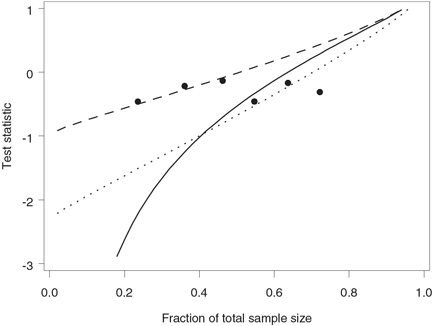
Figure 4.27 compares the Lan-Simon-Halperin and Pepe-Anderson-Betensky stopping boundaries with γ = 0.8 on an event rate scale. As in Figure 4.25, the resulting boundaries resemble straight-line segments parallel to the identity line. We can see from Figure 4.27 that the Lan-Simon-Halperin test is less likely to lead to early stopping at the first interim look compared to the Pepe-Anderson-Betensky tests with c = 1 and c = 2.326. However, the three stopping boundaries are pretty close to each other by the last look.
4.3.2 Futility Rules Based on Predictive Power
One of the important limitations of adaptive conditional power tests is that conditional power is computed assuming the observed treatment difference and standard deviation for the remainder of the trial. The observed treatment effect and its variability essentially serve as a prediction tool; however, no adjustment is made to account for the associated prediction error. This feature of the adaptive conditional power approach needs to be contrasted with corresponding features of predictive power methods discussed in this subsection. The predictive power methodology involves averaging the conditional power function (frequentist concept) with respect to the posterior distribution of the treatment effect given the observed data (Bayesian concept) and is frequently referred to as the mixed Bayesian-frequentist methodology. By using the posterior distribution we can improve our ability to quantify the uncertainty about future data; for instance, we can better account for the possibility that the current trend might be reversed.
Figure 4.27 Stopping boundaries of the Lan-Simon-Halperin test (—), Pepe-Anderson-Betensky test with c = 1 (- - -) and c = 2.326 (…), and interim survival rates (•) in the severe sepsis trial example. The futility index γ is 0.8; the continuation region is below the stopping boundary.
To define the predictive power approach, consider again a two-arm clinical trial with N patients per treatment group. An interim analysis is conducted after n patients have completed the trial in each group. Let Zn and ZN denote the test statistics computed at the interim and final analyses, respectively. The futility rule is expressed in terms of the following quantity:
Pn=∫Pn(δ)f(δ|Zn)dδ,
where δ is the treatment difference, Pn (δ) is the conditional power function defined in Section 4.3.1, i.e.,
Pn(δ)=P(ZN>z1−αwhen the treatment effect equals δ|Zn)=Φ(σ√nZn+(N−n)δ/√2−α√Nz1−ασ√N−n),
and f (δ|Zn) is the posterior density of the treatment difference δ given the data already observed. The defined quantity Pn can be thought of as the average conditional power and is termed the predictive power. The trial is terminated at the interim analysis due to lack of treatment benefit if the predictive power is less than 1 – γ for some prespecified futility index γ, and the trial continues otherwise.
As a side note, it is worth mentioning that one can also set up a predictive power test with a weight function based on the prior distribution of the treatment effect. This approach is similar to the basic conditional power approach in that it puts too much weight on original assumptions and ignores the interim data. Thus, it should not be surprising that predictive power tests based on the prior distribution are inferior to their counterparts relying on the posterior distribution of the treatment effect (Bernardo and Ibrahim, 2000).
Normally Distributed Endpoints
To illustrate the predictive power approach, we will begin with the case of normally distributed endpoints. Consider a two-arm clinical trial designed to compare an experimental drug to a control, and assume that the primary outcome variable is continuous and follows a normal distribution. The data will be analyzed at the final analysis using a z test and the null hypothesis of no treatment effect will be rejected if ZN > z1—α, where
ZN=√N/2(ˆμ1−ˆμ2)/s,
N is the sample seize per group, ˆμ1
Let μ1 and μ2 denote the mean treatment effects and σ denote the common standard deviation in the two groups, respectively. The prior knowledge about the mean treatment effects in each group is represented by a normal distribution; i.e., μ1 and μ2 are a priori assumed to be normally distributed with means μ*1 and μ*2, respectively, and common standard deviation σ*. Note that the difference between μ*1 and μ*2 is equal to the mean treatment difference under the alternative hypothesis.
As shown by Dmitrienko and Wang (2006), the predictive power conditional upon the interim test statistic Zn is given by
Pn=Φ(√NZn(1+an)+bn/σ−√nz1−α√N−nN[(N−n)(1−cn)+n]),
where
an=n−NN+N−nN(1+1n(σσ*)2)−1,bn=√n2N(N−n)(μ*1−μ*2)(1+n(σ*σ)2)−1,cn=(1+n(σ*σ)2)−1.
The trial will be stopped due to futility as soon as the computed predictive power falls below a prespecified threshold, i.e., as soon as Pn < 1 – γ. It is easy to invert this inequality and express the stopping rule in terms of the test statistic Zn:
Discontinue the trial due to lack of efficacy the first time Zn < ln,
with the adjusted critical value given by
ln=1√N(1+an)(√nz1−α+z1−γ√N−nN[(N−n)(1−cn)+n]−bn/α).
The derived formula for the predictive power involves the true standard deviation σ, which can be estimated by the pooled sample standard deviation. Also, the predictive power depends on the prior distributions of μ1 and μ2 only through the parameters an, bn and cn. These parameters measure the amount of prior information about the mean treatment difference and decrease in magnitude as the prior distributions of μ1 and μ2 become more spread out. In fact, it is easy to check that an, bn and cn approach zero as the common standard deviation of the priors increases in magnitude. Because of this, the formula for the predictive power simplifies significantly when we assume an improper uniform prior for both μ1 and μ2, i.e., let σ*→∞. In this case, the predictive power Pn is equal to
Φ(√NZn−√nz1−α√N−n),
and the adjusted critical value ln simplifies to
ln=√nNz1−α+√N−nnz1−γ.
Compared to the Lan-Simon-Halperin conditional power test introduced in Section 4.3.1, the unadjusted critical value z1—α in the formula for the predictive power is multiplied by √n/(N−n) instead of √N/(N−n). As pointed out by Geisser (1992), this implies that the predictive power approach to futility monitoring can exhibit a counterintuitive behavior at the early interim looks. To see what happens, note that n is small relative to N early in the trial and therefore the predictive power becomes virtually independent of z1—α. Although the futility rule based on predictive power is designed to assess the likelihood of a statistically significant outcome at the end of the trial, it no longer depends on the significance level α. It might be difficult to interpret an early decision to stop a clinical trial due to lack of efficacy because it is unclear what definition of efficacy is used in the futility rule.
Now that we have talked about futility rules associated with uniform priors, let us look at the other extreme and assume that the common standard deviation of the prior distributions of μ1 and μ2 is small.
It can be shown that in this case the predictive power asymptotically approaches the conditional power function evaluated at δ=μ*1−μ*2. If we assume that the difference between μ *1 and μ *2 equals the clinically significant difference, the predictive power is asymptotically equivalent to the Lan-Simon-Halperin test. This should come as little surprise, because assuming that μ*1 and μ*2 is very close to δ is another way of saying that the future data are generated from the alternative hypothesis.
We see that the choice of a prior distribution for the treatment difference can potentially impact predictive inferences, especially in small proof-of-concept trials; however, no consensus has been reached in the literature regarding a comprehensive prior selection strategy. For example, Spiegelhalter, Freedman and Blackburn (1986) recommended to use uniform prior distributions in clinical applications because they are quickly overwhelmed by the data and thus the associated predictive inferences are driven only by the observed data. Johns and Anderson (1999) also utilized decision rules based on a noninformative prior. In contrast, Herson (1979) stressed that a uniform prior is often undesirable because it assigns too much weight to extreme values of the treatment difference.
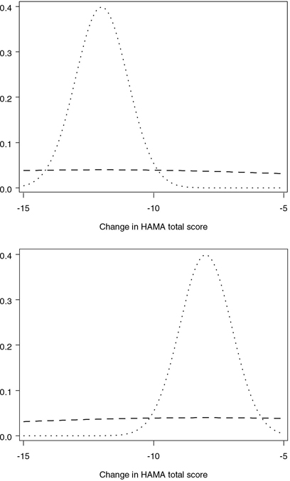
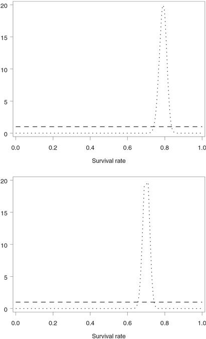
Elicitation of the prior distribution from clinical experts can be a complex and time-consuming activity; see Freedman and Spiegelhalter (1983) for a description of an elaborate interview of 18 physicians to quantify their prior beliefs about the size of the treatment effect in a clinical trial. Alternatively, one can utilize simple rules of thumb for selecting a prior distribution proposed in the literature. For example, Herson (1979) provided a set of guidelines for the selection of a prior distribution in the binary case. According to the guidelines, a beta prior with the coefficient of variation of 0.1 indicates a high degree of confidence, whereas the value of 0.5 corresponds to low confidence. A similar rule can be adopted to choose priors for the parameters of a normal distribution. For example, Table 4.13 presents two sets of parameters of normal priors in the generalized anxiety disorder trial. In both cases the means of the prior distributions are equal to the expected changes in the HAMA total score in the two treatment groups—i.e., —12 in the experimental group and —8 in the placebo group. The common standard deviation is chosen in such a way that the coefficient of variation with respect to the average HAMA change is equal to 0.1 or 1. The prior distributions in the experimental and placebo groups are displayed in Figure 4.28.
Table 4.13 Parameters of the normal prior for the mean changes in the HAMA score in the generalized anxiety disorder trial
| Experimental group | Placebo group | ||||
| Normal prior distribution | Mean | SD | Mean | SD | |
| “Low confidence” prior | –12 | 10 | –8 | 10 | |
| (coefficient of variation=1) | |||||
| “High confidence” prior | –12 | 1 | –8 | 1 | |
| (coefficient of variation=0.1) | |||||
%BayesFutilityCont Macro
The predictive power approach to futility monitoring in clinical trials with a normally distributed endpoint can be implemented using the %BayesFutilityCont macro provided in the Appendix. Note that the macro also supports the predictive probability approach introduced later in Section 4.3.3.
The %BayesFutilityCont macro has the following arguments:
• DATA is the name of the input data set with one record per interim look. The data set must include the following variables:
– N1 and N2 are the numbers of patients in the experimental and placebo groups included in the analysis data set at the current interim look.
– MEAN1 and MEAN2 are the estimates of the mean treatment effects in the experimental and placebo groups at the current interim look.
– SD1 and SD2 are the sample standard deviations in the experimental and placebo groups at the current interim look.
• PAR is the name of the single-record input data set with the following variables:
– NN1 and NN2 are the projected numbers of patients in the experimental and placebo groups.
– MU1, MU2 and SIGMA are the means and common standard deviation of the prior distributions of the mean treatment effects in the experimental and placebo groups.
• DELTA is the clinically significant difference between the treatment groups. This parameter is required by the Bayesian predictive probability method and is ignored by the predictive power method.
• ETA is the confidence level of the Bayesian predictive probability method. This parameter is required by the Bayesian predictive probability method and is ignored by the predictive power method.
• ALPHA is the one-sided Type I error probability of the significance test carried out at the end of the trial. This parameter is required by the predictive power method and is ignored by the Bayesian predictive probability method.
• PROB is the name of the data set containing the predictive power and predictive probability at each interim look. This data set is generated by the macro and includes the following variables: – ANALYSIS is the analysis number.
– FRACTION is the fraction of the total sample size.
– PREDPOWER is the computed predictive power (predictive power method).
– PREDPROB is the computed predictive probability (Bayesian predictive probability method).
Figure 4.28 Low confidence (- - -) and high confidence (…) prior distributions of the mean change in the HAMA total score in the generalized anxiety disorder trial example. Upper panel: experimental group (Mean HAMA change is assumed to be —12); lower panel: placebo group (Mean HAMA change is assumed to be —8).
Program 4.21 utilizes the %BayesFutilityCont macro to carry out the predictive power test in the generalized anxiety disorder trial. The futility rule is constructed using the two sets of prior distributions displayed in Table 4.13. The parameters of the priors are included in the LOWCONF and HIGHCONF data sets. The data sets also include the projected sample sizes NN1 and NN2 of 41 patients per treatment group. The futility analysis is performed with a one-sided significance level ALPHA=0.1. The DELTA and ETA parameters of the %BayesFutilityCont macro are intended for predictive probability inferences and are not used in predictive power calculations.
To facilitate the comparison of the predictive and conditional power approaches, Program 4.21 also carries out the Lan-Simon-Halperin test for the same set of interim results by calling the %CondPowerLSH macro. Note that the %CondPowerLSH macro requires the specification of the effect size under the alternative hypothesis. Since the treatment difference and the standard deviation of HAMA changes were assumed to be 4 and 8.5 in the sample size calculation, the effect size is 4/8.5 = 0.4706.
Lastly, the %BayesFutilityCont macro, as well all other SAS macros introduced in this chapter, assumes that a positive treatment difference indicates improvement compared to the placebo. Since the experimental drug improves the HAMA total score by decreasing it, the treatment difference is defined in Program 4.21 as the mean HAMA change in the placebo group minus the mean HAMA change in the experimental group.
Program 4.21 Predictive power test in the generalized anxiety disorder trial
data genanx;
input n1 mean1 sd1 n2 mean2 sd2;
datalines;
| 11 | -8.4 | 6.4 | 10 | -9.2 | 7.3 |
| 20 | -8.1 | 6.9 | 20 | -9.4 | 6.7 |
| 30 | -9.1 | 7.7 | 31 | -8.9 | 7.4 |
| ; | |||||
data lowconf;
input nn1 nn2 mu1 mu2sigma;
datalines;
41 41 -8 -12 10
;
data highconf;
input nn1 nn2 mu1 mu2 sigma;
datalines;
41 41 -8 -12 1
;
%BayesFutilityCont(data=genanx,par=lowconf,delta=0,eta=0.9,alpha=0.1,
prob=lowout);
%BayesFutilityCont(data=genanx,par=highconf,delta=0,eta=0.9,alpha=0.1,
prob=highout);
proc print data=lowout noobs label;
title "Predictive power test, Low confidence prior";
var Analysis Fraction PredPower;
proc print data=highout noobs label;
title "Predictive power test, High confidence prior";
var Analysis Fraction PredPower;
data test;
set genanx;
s=sqrt(((n1-1)*sd1*sd1+(n2-1)*sd2*sd2)/(n1+n2-2));
teststat=(mean1-mean2)/(s*sqrt(1/n1+1/n2));
n=(n1+n2)/2;
keep n teststat;
%CondPowerLSH(data=test,effsize=0.4706,alpha=0.1,gamma=0.8,nn=41,
prob=out,boundary=boundary);
proc print data=out noobs label;
title "Conditional power test";
var Analysis Fraction CondPower;
run;
Output from Program 4.21
Predictive power test, Low confidence prior
| Analysis | Fraction of total sample size |
Predictive power |
| 1 | 0.26 | 0.3414 |
| 2 | 0.49 | 0.3490 |
| 3 | 0.74 | 0.0088 |
Predictive power test, High confidence prior
| Analysis | Fraction of total sample size |
Predictive power |
| 1 | 0.26 | 0.6917 |
| 2 | 0.49 | 0.6087 |
| 3 | 0.74 | 0.0335 |
| Conditional power test | ||
| Analysis | Fraction of total sample size |
Predictive power |
| 1 | 0.26 | 0.6946 |
| 2 | 0.49 | 0.6271 |
| 3 | 0.74 | 0.0515 |
Output 4.21 displays the probabilities of a positive final outcome produced by the predictive and conditional power methods in the generalized anxiety disorder trial. Comparing the predictive power values associated with the low and high confidence priors, we see that the probability of observing a statistically significant result at the planned termination point is considerably higher when the variance of the prior is assumed to be small. This difference, however, does not affect the decision-making process. The predictive power is consistently above the 20% threshold at the first two looks, which suggests that the trial should continue, and falls below 5% at the third look. Given the low probability of success, it is prudent to discontinue the trial at the third interim inspection due to lack of efficacy.
The conditional power shown in the bottom part of Output 4.21 is quite close to the predictive power under the high confidence prior. This is because the predictive power method approximates the conditional power method as the prior information about the treatment difference becomes more precise. Since predictive power tests based on very strong priors assume that the future data are generated from the alternative hypothesis, they tend to produce an overly optimistic prediction about the final trial outcome.
Figure 4.29 displays the stopping boundaries of the predictive power test based on the low and high confidence priors as well as the boundary of the Lan-Simon-Halperin test. The boundaries have been generated by a program similar to Program 4.17. Figure 4.29 demonstrates the relationship between the amount of prior information about the treatment effect and the probability of early termination due to lack of benefit. An assumption of a weak prior increases the chances of an early termination. For example, with the low confidence prior, a trial will be stopped almost immediately if the observed z statistic is less than —0.5. In contrast, the test based on the high confidence prior (as well as the Lan-Simon-Halperin test) will consider this z statistic somewhat consistent with the alternative hypothesis in the first part of the trial. Clinical researchers need to keep this relationship in mind when selecting a futility rule based on predictive power.
Figure 4.29 Stopping boundaries of the Lan-Simon-Halperin test (—), predictive test based on a low confidence prior (- - -) and high confidence prior (…) and interim z statistics (•) in the generalized anxiety disorder trial example. The futility index γ is 0.8; the continuation region is above the stopping boundary.
Binary Endpoints
In order to introduce predictive power futility rules for clinical trials with binary outcomes, we will return to the severe sepsis trial example. Before defining the predictive power test, it is instructive to point out an important difference between conditional and predictive power methods for binary data. Recall that conditional power tests in Section 4.3.1 rely on the asymptotic normality of z statistics and therefore can be applied to clinical trials with both continuous and binary variables. By contrast, the case of binary endpoints needs to be considered separately within the predictive power framework because predictive inferences are based on the Bayesian paradigm. Although a normal approximation can be used in the calculation of the conditional power function, one still needs to define prior distributions for event rates in the experimental and control groups. In this subsection we will derive an exact formula for the predictive power in the binary case that does not rely on a normal approximation; see Dmitrienko and Wang (2006) for more details.
Let π1 and π2 denote the survival rates in the experimental and placebo groups, and let Bi and Ai denote the number of patients who survived to the end of the 28-day study period in Treatment group i before and after the interim look, respectively. Efficacy of the experimental drug will be established at the final analysis if the test statistic
Zn=(p1−p2)/√2ˉp(1−ˉp)/N
is significant at a one-sided α level. Here p1 and p2 are estimated survival rates in the experimental and placebo groups and ˉp is the average survival rate; i.e.,
pi=Bi+AiN, i=1,2, ˉp=(p1+p2)/2.
The event counts B1 and B2 are computed from the interim data; however, the future event counts A1 and A2 are unobservable and, in order to compute ZN, we will need to rely on their predicted values. Assume that πi follows a beta distribution with the parameters αi and βi. Given Bi, the predicted value of Ai follows a beta-binomial distribution; i.e.,
pi(a|b)=P(Ai=a|Bi=b)=Γ(N−n+1)B(b+a+αi,N−b−a+βi)Γ(N−n−a+1)Γ(a+1)B(b+αi,n−b+βi),
where 0 ≤ a ≤ N — n, and () and B () are the gamma and beta functions.
Now that we have derived the predictive distribution of the future event counts A1 and A2, the predictive probability of a statistically significant difference at the planned end of the trial is given by
Pn=N−n∑j=0N−n∑k=0I(ZN>z1−α|A1=j, A2=k)p1(j|B1)p2(k|B2).
Here I () is the indicator function and thus the predictive probability Pn is computed by summing over the values of A1 and A2 that result in a significant test statistic ZN. The trial is terminated at the interim analysis due to futility if the predictive probability of a positive trial outcome is sufficiently small.
Table 4.14 Prior distribution of 28-day survival rates in the severe sepsis trial
| Experimental group | Placebo group | |||||
| Beta prior distribution | α | β | α | β | ||
| “Low confidence” prior (uniform prior with coefficient of variation=0.58) |
1 | 1 | 1 | 1 | ||
| “High confidence” prior (coefficient of variation=0.025) |
335 | 89 | 479 | 205 | ||
Table 4.14 shows two sets of prior distributions of 28-day survival corresponding to low and high confidence scenarios. The calculations assumed that the 28-day survival rates in the experimental and placebo groups are equal to 79% and 70%, respectively. The prior distributions were chosen using a version of the Herson rule. As was mentioned previously, Herson (1979) proposed a simple rule to facilitate the selection of prior distributions in clinical trials with a binary response variable:
• “Low confidence” prior: Beta distribution with the mean equal to the expected event rate (e.g., expected 28-day survival rate) and coefficient of variation equal to 0.5
• “Medium confidence” prior: Beta distribution with the mean equal to the expected event rate and coefficient of variation equal to 0.25
• “High confidence” prior: Beta distribution with the mean equal to the expected event rate and coefficient of variation equal to 0.1.
Once the mean m and coefficient of variation c of a beta distribution have been specified, its parameters are given by
α=(1−m)/c2−m, β=α(1−m)/m.
In practice, one often needs to slightly modify the described rule. First, the Herson rule is applicable to event rates ranging from 0.3 to 0.7. Outside of this range, it may not be possible to achieve the coefficient of variation of 0.5, or even 0.25, with a bell-shaped beta distribution, and U-shaped priors are clearly undesirable in practice. For this reason, a uniform prior was selected to represent a low confidence scenario in the severe sepsis trial. Further, even prior distributions with the coefficient of variation around 0.1 are fairly weak and are completely dominated by the data in large trials. To specify high confidence priors in the severe sepsis trial, we set the coefficient of variation to 0.025. The obtained prior distributions are depicted in Figure 4.30.
%BayesFutilityBin Macro
Program 4.22 performs predictive power calculations in the severe sepsis trial by invoking the %BayesFutilityBin macro included in the Appendix. The macro implements the predictive power method based on the mixed Bayesian-frequentist approach as well as the fully Bayesian predictive method that will be described later in Section 4.3.3. Here we will focus on predictive power inferences to examine early evidence of futility in the severe sepsis trial.
The %BayesFutilityBin macro has the following arguments:
• DATA is the name of the input data set with one record per interim look. The data set must include the following variables:
– N1 and N2 are the numbers of patients in the experimental and placebo groups included in the analysis data set at the current interim look.
– COUNT1 and COUNT2 are the observed event counts in the experimental and placebo groups at the current interim look.
• PAR is the name of the single-record input data set with the following variables:
– NN1 and NN2 are the projected numbers of patients in the experimental and placebo groups.
– ALPHA1 and ALPHA2 are the α parameters of beta priors for event rates in the experimental and placebo groups.
– BETA1 and BETA2 are the β parameters of beta priors for event rates in the experimental and placebo groups.
• DELTA is the clinically significant difference between the treatment groups. This parameter is required by the Bayesian predictive probability method and is ignored by the predictive power method.
• ETA is the confidence level of the Bayesian predictive probability method. This parameter is required by the Bayesian predictive probability method and is ignored by the predictive power method.
• ALPHA is the one-sided Type I error probability of the significance test carried out at the end of the trial. This parameter is required by the predictive power method and is ignored by the Bayesian predictive probability method.
• PROB is the name of the data set containing the predictive power and predictive probability at each interim look. This data set includes the same four variables as the output data set in the %BayesFutilityCont macro, i.e., ANALYSIS, FRACTION, PREDPOWER and PREDPROB.
Figure 4.30 Low confidence (- - -) and high confidence (…) prior distributions of 28-day survival rates in the severe sepsis trial example. Upper panel: experimental group (28-day survival rate is assumed to be 79%); lower panel: placebo group (28-day survival rate is assumed to be 70%).
In order to assess the amount of evidence in favor of the experimental drug at each interim look, Program 4.22 computes the predictive power using the prior distributions of 28-day survival rates shown in Table 4.14. The parameters of these beta distributions, included in the LOWCONF and HIGHCONF data sets, are passed to the %BayesFutilityBin macro. The one-sided significance level ALPHA is 0.1 and the projected sample sizes NN1 and NN2 are set to 212 patients. The DELTA and ETA parameters are not used in predictive power calculations and are set to arbitrary values.
Output 4.22 summarizes the results of predictive power inferences performed at each of the six looks in the severe sepsis trial. As in the case of normally distributed endpoints, the use of less informative priors increases the chances to declare futility. Output 4.22 shows that, with the low confidence prior, the probability of eventual success is 11.1% at the first look, which is substantially less than 22.8% Pepe-Anderson-Betensky test with c = 1 in Output 4.20) or 55.5% (Lan-Simon-Halperin test in Output 4.17). As a result, the futility rule is met at the very first interim analysis.
Program 4.22 Predictive power test in the severe sepsis trial
data sevsep2;
input n1 count1 n2 count2;
datalines;
| 55 | 33 | 45 | 29 |
| 79 | 51 | 74 | 49 |
| 101 | 65 | 95 | 62 |
| 117 | 75 | 115 | 77 |
| 136 | 88 | 134 | 88 |
| 155 | 99 | 151 | 99 |
| ; | |||
data LowConf;
input nn1 nn2 alpha1 alpha2 beta1 beta2;
datalines;
212 212 1 1 1 1
;
data HighConf;
input nn1 nn2 alpha1 alpha2 beta1 beta2;
datalines;
212 212 335 479 89 205
;
%BayesFutilityBin(data=sevsep2,par=LowConf,delta=0,eta=0.9,
alpha=0.1,prob=LowProb);
%BayesFutilityBin(data=sevsep2,par=HighConf,delta=0,eta=0.9,
alpha=0.1,prob=HighProb);
proc print data=LowProb noobs label;
title "Low confidence prior";
var Analysis Fraction PredPower;
proc print data=HighProb noobs label;
title "High confidence prior";
var Analysis Fraction PredPower;
run;
Output from Program 4.22
| Low confidence prior | ||||
| Analysis | Fraction of total sample size |
Predictive power |
||
| 1 | 0.24 | 0.1107 | ||
| 2 | 0.36 | 0.1091 | ||
| 3 | 0.46 | 0.0864 | ||
| 4 | 0.55 | 0.0183 | ||
| 5 | 0.64 | 0.0243 | ||
| 6 | 0.72 | 0.0041 | ||
| High confidence prior | ||||
| Analysis | Fraction of total sample size |
Predictive power |
||
| 1 | 0.24 | 0.3349 | ||
| 2 | 0.36 | 0.3012 | ||
| 3 | 0.46 | 0.2023 | ||
| 4 | 0.55 | 0.0652 | ||
| 5 | 0.64 | 0.0579 | ||
| 6 | 0.72 | 0.0087 | ||
Selecting a more informative prior increases the probability of success at the first interim analysis to 33.5% and brings the predictive power test closer to the Lan-Simon-Halperin conditional power test. However, even in this setting the predictive power drops below the 20% threshold at the fourth look, indicating that a decision to discontinue the patient enrollment should have been considered early in the trial.
4.3.3 Futility Rules Based on Predictive Probability
As we explained in the previous subsection, predictive power tests are derived by averaging the conditional power function with respect to the posterior distribution of the treatment difference given the already observed data. Several authors have indicated that predictive power tests are based on a mixture of Bayesian and frequentist methods and therefore “neither Bayesian nor frequentist statisticians may be satisfied [with them]” (Jennison and Turnbull, 1990), and “the result does not have an acceptable frequentist interpretation and, furthermore, this is not the kind of test a Bayesian would apply” (Geisser and Johnson, 1994).
This section introduces an alternative approach to Bayesian futility monitoring known as the predictive probability approach. Roughly speaking, predictive probability tests are constructed by replacing the frequentist component of predictive power tests (conditional power function) with a Bayesian one (posterior probability of a positive trial outcome). The predictive probability approach is illustrated below using examples from clinical trials with normally distributed and binary response variables.
Normally Distributed Endpoints
As we indicated above, a positive trial outcome is defined within the Bayesian predictive probability framework in terms of the posterior probability of a clinically important treatment effect rather than statistical significance. To see how this change affects futility testing in clinical applications, consider a trial comparing an experimental drug to a placebo and assume that its primary endpoint is a continuous, normally distributed variable.
The trial will be declared positive if one demonstrates that the posterior probability of a clinically important improvement is greater than a prespecified confidence level η; i.e.,
P (μ1 — μ2 > δ|observed data) > η,
where μ1 and μ2 denote the mean treatment effects in the two treatment groups, δ is a clinically significant treatment difference, and 0 < η < 1. Note that η is typically greater than 0.8, and choosing a larger value of the confidence level reduces the likelihood of a positive trial outcome. The treatment difference δ can either be a constant or be expressed in terms of the standard deviation, in which case the introduced criterion becomes a function of the effect size (μ1 — μ2)/σ (here σ denotes the common standard deviation in the two treatment groups).
In order to predict the probability of a positive trial outcome from the data available at an interim analysis, we will employ a trick similar to the one we used in the derivation of the predictive power test for binary endpoints in Section 4.3.2. In broad strokes, the data collected before the interim analysis are used to predict future data, which are then combined with the observed data to estimate the posterior probability of a clinically significant treatment difference.
Assume that the mean treatment effects μ1 and μ2 are normally distributed with means μ*1 and μ*2 and standard deviation σ*. As stated by Dmitrienko and Wang (2006), the predictive probability of observing a clinically significant treatment difference upon termination given the interim test statistic Zn is equal to
Pn=Φ(√NZn(1−an)+bn/σ−(δ/σ)√nN/2−√nzη(1−CN)√N−nN(1−aN)2[(N−n)(1−an)+n]),
where
an=(1+n(σ*σ)2)−1,bn=√nN2(μ*1−μ*2)(1+n(σ*σ)2)−1,cn=1−(1+1n(σσ*)2)−1.
The trial will be stopped in favor of the null hypothesis of no treatment effect as soon as the predictive probability falls below 1 – γ.
As in Section 4.3.2, the unknown standard deviation σ can be estimated using the pooled sample standard deviation. The parameters an, bn and cn quantify the amount of prior information about the mean treatment effects μ1 and μ2. The three parameters converge to zero as σ*→∞ i.e., as the prior information becomes less precise. The limiting value of the predictive probability corresponding to the case of uniform priors is given by
Pn=Φ(√NZn−√nzη−(δ/σ)√nN/2√(N−n)).
Comparing this formula to the formula for the predictive power derived in Section 4.3.2, we see that the predictive probability method can be thought of as a “mirror image” of the predictive power method when the clinically significant treatment difference δ is set to 0. Indeed, assuming a uniform prior andδ = 0, it is easy to verify that the two methods become identical when η = 1 — α. For example, a predictive probability test with a 90% confidence level (η = 0.9) is identical to a predictive power test with a one-sided 0.1 level (α = 0.1).
Looking at the case of a small common variance of the prior distributions of μ1 and μ2, it is easy to demonstrate that the predictive probability test is asymptotically independent of the test statistic Zn and thus it turns into a deterministic rule. Specifically, the predictive probability converges to 1 if μ*1−μ*2>δ and 0 otherwise. As a result, a predictive probability test will trigger an early termination of the trial regardless of the size of the treatment difference as long as the selected prior distributions meet the condition μ*1−μ*2≤δ. Due to this property, it is advisable to avoid strong prior distributions when setting up futility rules based on the predictive probability method.
Program 4.23 explores the relationship between the magnitude of the clinically significant treatment difference δ and predictive probability of a positive final outcome in the generalized anxiety disorder trial. To save space, we will focus on the low confidence priors for the mean HAMA changes displayed in Table 4.13. The calculations can be easily repeated for the high confidence priors or any other set of prior distributions.
The predictive probability is computed in Program 4.23 by invoking the %BayesFutilityCont macro with DELTA=1, 2 and 3 and ETA=0.9. The chosen value of the confidence level η corresponds to a one-sided significance level of 0.1 in the predictive power framework. Note that the ALPHA parameter will be ignored in predictive probability calculations.
Program 4.23 Predictive probability test in the generalized anxiety disorder trial
%BayesFutilityCont(data=genanx,par=lowconf,delta=1,eta=0.9,
alpha=0.1,prob=delta1);
%BayesFutilityCont(data=genanx,par=lowconf,delta=2,eta=0.9,
alpha=0.1,prob=delta2);
%BayesFutilityCont(data=genanx,par=lowconf,delta=3,eta=0.9,
alpha=0.1,prob=delta3);
proc print data=delta1 noobs label;
title "Delta=1";
var Analysis Fraction PredProb;
proc print data=delta2 noobs label;
title "Delta=2";
var Analysis Fraction PredProb;
proc print data=delta3 noobs label;
title "Delta=3";
var Analysis Fraction PredProb;
run;
Output from Program 4.23
| Delta=1 | ||||
| Analysis | Fraction of total sample size |
Predictive probability |
||
| 1 | 0.26 | 0.2135 | ||
| 2 | 0.49 | 0.1523 | ||
| 3 | 0.74 | 0.0004 | ||
| Delta=2 | ||||
| Analysis | Fraction of total sample size |
Predictive probability |
||
| 1 | 0.26 | 0.1164 | ||
| 2 | 0.49 | 0.0458 | ||
| 3 | 0.74 | 0.0000 | ||
| Delta=3 | ||||
| Analysis | Fraction of total sample size |
Predictive probability |
||
| 1 | 0.26 | 0.0556 | ||
| 2 | 0.49 | 0.0094 | ||
| 3 | 0.74 | 0.0000 | ||
Output 4.23 shows the predictive probability of observing a 1-, 2- and 3-point improvement (DELTA parameter) in the mean HAMA change compared to the placebo at each of the three interim looks. As expected, the predictive probability declines quickly with the increasing DELTA parameter. Consider, for example, the first interim analysis. The predictive probability of observing a 1-point mean treatment difference at the end of the trial is 21.4%, whereas the predictive probability for 2-and 3-point differences are equal to 11.6% and 5.6%, respectively. The findings suggest that it is no longer worthwhile continuing the trial to its planned end if one is interested in detecting a substantial amount of improvement over the placebo.
Binary Endpoints
The predictive probability framework introduced in the previous subsection is easily extended to the case of binary outcome variables. Consider again the severe sepsis trial example and let p1 and p2 denote the 28-day survival rates in the experimental and placebo groups. The trial will be declared successful at the final analysis if the probability of a clinically meaningful difference in survival rates exceeds a prespecified confidence level η; i.e.,
P(p1−p2>δ|observed data)>η,
where δ denotes a clinically significant treatment difference.
As in the normal case, the posterior probability of p1 — p2 > δ depends both on the interim and future data. Let Bi and Ai denote the event counts in treatment group i at the interim analysis and between the interim and final analyses, respectively. Since the future event counts A1 and A2 are not available to the clinical researchers at the time the interim analysis is performed, they will be replaced by their predicted values. The predicted values of A1 and A2 are computed from B1 and B2 as well as prior distributions of the survival rates p1 and p2 and, as shown in Section 4.3.2, follow a beta-binomial distribution. Given the predicted values, it is easy to prove that the posterior distribution of the survival rates p1 and p2 is beta with the parameters
α*i=Bi+Ai+αi, β*i=N−Bi−Ai−βi.
Now that all of the individual ingredients have been obtained, we can compute the predictive probability of a positive trial outcome given the data observed at the interim look (Dmitrienko and Wang, 2006):
Pn=N−n∑j=0N−n∑k=0I(P(p*1−p*2>δ|Α1=j, A2=k)>η)p1(j|B1)p2(k|B2),
where I () is an indicator function and asterisks indicate that the probability is computed with respect to the posterior distribution of the survival rates p1 and p2. Put simply, the predictive probability is obtained by summing over all possible values of future event counts for which the posterior probability of p1 — p2 > δ is greater than the prespecified threshold η. Configurations of future event counts that do not lead to a positive trial outcome are automatically excluded from the calculation. The experimental drug will be considered futile and patient enrollment will be stopped as soon as Pn < 1 – γ.
The value of
P(p*1−p*2>δ|Α1=j, A2=k)
can be computed exactly by taking advantage of the fact that p*1 and p*2 are independent random variables with a beta distribution:
P(p*1−p*2>δ|Α1=j, A2=k)
=1B(α*1,β*1)∫1δpα*1−1(1−p)β*1−1FB(α*2,β*2)(p−δ)dp,
where FB(α*2,β*2)) is the cumulative distribution function of a B(α*2,β*2)) distribution. The integral in this formula can be computed using any numerical integration routine. The %BayesFutilityBin macro that implements the outlined futility testing method relies on the QUAD function in the SAS/IML library.
Program 4.24 performs predictive probability calculations in the severe sepsis trial by utilizing the %BayesFutilityBin macro. We are interested in computing the predictive probability of observing any improvement in 28-day survival as well as observing a 5% and 10% absolute increase in 28-day survival at the end of the trial. Therefore the DELTA parameter will be set to 0, 0.05 and 0.1. The confidence level of the Bayesian predictive probability test (ETA parameter) is equal to 0.9. The calculations will be performed for the set of low confidence priors shown in Table 4.14. Lastly, as in Program 4.23, the ALPHA parameter will be ignored in predictive probability calculations.
Program 4.24 Predictive probability test in the severe sepsis trial
%BayesFutilityBin(data=sevsep2,par=lowconf,delta=0,eta=0.9,
alpha=0.1,prob=delta1);
%BayesFutilityBin(data=sevsep2,par=lowconf,delta=0.05,eta=0.9,
alpha=0.1,prob=delta2);
%BayesFutilityBin(data=sevsep2,par=lowconf,delta=0.1,eta=0.9,
alpha=0.1,prob=delta3);
proc print data=delta1 noobs label;
title "Delta=0";
var Analysis Fraction PredProb;
proc print data=delta2 noobs label;
title "Delta=0.05";
var Analysis Fraction PredProb;
proc print data=delta3 noobs label;
title "Delta=0.1";
var Analysis Fraction PredProb;
run;
Output from Program 4.24
| Delta=0 | ||||
| Analysis | Fraction of total sample size |
Predictive probability |
||
| 1 | 0.24 | 0.1099 | ||
| 2 | 0.36 | 0.1088 | ||
| 3 | 0.46 | 0.0862 | ||
| 4 | 0.55 | 0.0183 | ||
| 5 | 0.64 | 0.0243 | ||
| 6 | 0.72 | 0.0041 | ||
| Delta=0.05 | ||||
| Analysis | Fraction of total sample size |
Predictive probability |
||
| 1 | 0.24 | 0.0341 | ||
| 2 | 0.36 | 0.0190 | ||
| 3 | 0.46 | 0.0081 | ||
| 4 | 0.55 | 0.0004 | ||
| 5 | 0.64 | 0.0002 | ||
| 6 | 0.72 | 0.0000 | ||
| Delta=0.1 | ||||
| Analysis | Fraction of total sample size |
Predictive probability |
||
| 1 | 0.24 | 0.0074 | ||
| 2 | 0.36 | 0.0019 | ||
| 3 | 0.46 | 0.0003 | ||
| 4 | 0.55 | 0.0000 | ||
| 5 | 0.64 | 0.0000 | ||
| 6 | 0.72 | 0.0000 | ||
Output 4.24 lists predictive probability values computed at each of the six interim looks under three choices of the DELTA parameter. Recall from the beginning of this section that, for normally distributed outcomes, the predictive probability test is closely related to the predictive power test when η = 1 — α and the clinically meaningful treatment difference δ is set to 0. A similar relationship is observed in the binary case as well. We see from Output 4.24 that the predictive probabilities with DELTA=0 are virtually equal to the predictive power values with α = 0.1 shown under “Low confidence prior” in Output 4.22. Therefore, the constructed predictive probability test will roughly correspond to the predictive power test with a one-sided significance level of 0.1.
We also see from Output 4.24 that larger values of the clinically meaningful treatment difference δ are associated with lower predictive probabilities of a positive trial outcome. For example, if one would like to demonstrate with a 90% confidence that the experimental drug improves the 28-day survival rate by 5% or 10% (in absolute terms), the predictive probability of a positive trial outcome at the very first interim look drops to 3.4% and 0.7%, respectively. It appears prudent to suspend the patient enrollment at the first look, because the negative conclusion is unlikely to change even if the trial continued to the planned end.
4.3.4 Summary
This section reviewed three approaches to constructing futility testing procedures in clinical trials: frequentist conditional power methods, mixed Bayesian-frequentist methods based on predictive power, and Bayesian predictive probability methods. These futility tests are often collectively referred to as stochastic curtailment tests because they rely on stochastic arguments in order to decide when to curtail sampling. Specifically, a clinical trial is terminated at an interim analysis when the observed data indicate that it is highly unlikely that the experimental drug would separate from the control at the end of the study. The three families of futility tests differ in how they define separation between treatment arms:
• Conditional power tests reviewed in the section can be further subdivided into basic and adaptive conditional power tests. Both methods evaluate the probability of observing a statistically significant treatment difference at the planned end of the trial given the interim data. Basic conditional power procedures (e.g., Lan-Simon-Halperin test) rely heavily on the hypothesized value of the treatment effect, whereas adaptive conditional power procedures (e.g., Pepe-Anderson-Betensky test) are based on a sample estimate of the treatment difference to predict the distribution of the future data. For this reason, adaptive tests are generally more appealing in clinical trial applications than tests tied to an assumed value of the treatment difference. The basic and adaptive conditional power methods can be implemented using the %CondPowerLSH and %CondPowerPAB macros described in this section.
• Predictive power tests extend the adaptive approach further by incorporating more data-driven elements into the decision rule. This is achieved by averaging the conditional power function with respect to a posterior distribution of the treatment difference. The clinical trial is terminated as soon as the average conditional power (known as the predictive power) falls below a certain threshold. An assumed prior distribution of the mean treatment difference can have great influence on the resulting futility rule. Selecting a noninformative prior that is quickly dominated by the data increases the chances of early stopping due to futility. On the other hand, with a strong prior distribution, a predictive power test is asymptotically equivalent to a frequentist conditional power test and thus is generally less sensitive to negative trends in the data. The section introduced two SAS macros (%BayesFutilityCont and %BayesFutilityBin macros) for carrying out predictive power tests in clinical trials with normally distributed and binary endpoints.
• Predictive probability tests provide a fully Bayesian solution to the futility testing problem. Within the predictive probability framework, a positive trial outcome is defined in terms of the posterior probability of a clinically important treatment effect rather than statistical significance. Under a noninformative prior, predictive probability tests yield results similar to those produced by predictive power tests and turn into deterministic rules when the variance of the prior distribution is small. For this reason, it is advisable to avoid strong priors when setting up futility rules based on the predictive probability method. Bayesian predictive probability inferences can be performed using the %BayesFutilityCont and %BayesFutilityBin macros.
Although the Type II error rate of trial designs with futility monitoring is greater than the nominal value, adjustments are rarely done in practice. This is due mainly to the fact that stochastic curtailment tests minimize the probability of early termination compared to their group sequential counterparts.
Finally, due to their simplicity, futility tests reviewed in this section may be more appealing in practice than computationally complex futility monitoring strategies based on error spending functions. In addition, the futility boundary of a group sequential design depends heavily on the assumed value of the treatment difference, which may no longer be supported by the data. Therefore, the repeated significance approach is less robust than stochastic curtailment approaches such as the adaptive conditional power or Bayesian methods described in this section.
1 As shown by Jennison and Turnbull (2000, Chapter 13), the group sequential designs and sequential monitoring strategies discussed later in this section are easily extended to the case of time-to-event variables. An interesting feature of group sequential tests in clinical trials with time-to-event endpoints that differentiates them from normally distributed and binary endpoints is a repeated use of data collected from the same patient. For example, in survival trials, the test statistic at each interim look is computed from all survival times (either observed or censored) and thus any patient who survives to the end of the study contributes to every interim test statistic.
2 This treatment difference is equal to √2/n,, where c is the adjusted critical value, σ is the common standard deviation, and n is the sample size per group. In this case, c = 2.8626, σ = 8, and n = 77. Therefore, the detectable treatment difference is 3.69.
3 Although the paper by Pampallona, Tsiatis and Kim was published in 2001, it was actually written prior to 1994.
4 In the case of simultaneous monitoring of efficacy and futility, the prespecified stopping boundaries are converted into α- and β-spending functions.
5 Dr. KyungMann Kim introduced this family in his Ph.D. dissertation in 1986 at the University of Wisconsin at Madison.
6 Other error spending functions corresponding to the O’Brien-Fleming plan can be requested in a similar manner. For example, let SPFUNCTION=3 and SPRHO=0 to specify a Lan-DeMets error spending function or let SPFUNCTION=4 and SPRHO=3 to request a Jennison-Turnbull error spending function.
7 The SPRHO parameter may need to be changed as well when using Lan-DeMets, Jennison-Turnbull or Hwang-Shih-DeCani error spending functions. For example, to specify a Lan-DeMets error spending function corresponding to the Pocock plan, let SPFUNCTION=3 and SPRHO=0.5.
8 To see why the lower limit of the confidence intervals is based on the upper stopping boundary and vice versa, note that the confidence intervals are defined to be consistent with the group sequential decision rule. For example, H0 is rejected if Zk > uk, which implies that ˆδk−uksk>0 0. In other words, the lower confidence limit for the treatment difference excludes 0 when the group sequential test rejects the null hypothesis of no treatment difference. Likewise, Zk < lk implies that the confidence interval lies completely below 0.