
Analysis of Stratified Data 1
1.5 Tests for Qualitative Interactions
This chapter discusses the analysis of clinical outcomes in the presence of influential covariates such as investigational center or patient demographics. The following analysis methods are reviewed:
• Stratified analyses of continuous endpoints using parametric methods based on fixed and random effects models as well as nonparametric methods.
• Simple randomization-based methods as well as more advanced exact and model-based methods for analyzing stratified categorical outcomes.
• Analysis of stratified time-to-event data using randomization-based tests and the Cox proportional hazards model.
The chapter also introduces statistical methods for studying the nature of treatment-by-stratum interactions in clinical trials.
1.1 Introduction
This chapter addresses issues related to adjustment for important covariates in clinical applications. The goal of an adjusted analysis is to provide an overall test of treatment effect in the presence of factors that have a significant effect on the outcome variable. Two different types of factors known to influence the outcome are commonly encountered in clinical trials: prognostic and non-prognostic factors (Mehrotra, 2001). Prognostic factors are known to influence the outcome variables in a systematic way. For instance, the analysis of survival data is always adjusted for prognostic factors such as a patient’s age and disease severity because these patient characteristics are strongly correlated with mortality. By contrast, non-prognostic factors are likely to impact the trial’s outcome but their effects do not exhibit a predictable pattern. It is well known that treatment differences vary, sometimes dramatically, across investigational centers in multicenter clinical trials. However, the nature of center-to-center variability is different from the variability associated with a patient’s age or disease severity. Center-specific treatment differences are dependent on a large number of factors, e.g., geographical location, general quality of care, etc. As a consequence, individual centers influence the overall treatment difference in a fairly random manner and it is natural to classify the center as a non-prognostic factor.
Adjustments for important covariates are carried out using randomization- and model-based methods (Koch and Edwards, 1988; Lachin, 2000, Chapter 4). The idea behind randomization-based analyses is to explicitly control factors influencing the outcome variable while assessing the relationship between the treatment effect and outcome. The popular Cochran-Mantel-Haenszel method for categorical data serves as a good example of this approach. In order to adjust for a covariate, the sample is divided into strata that are relatively homogeneous with respect to the selected covariate. The treatment effect is examined separately within each stratum and thus the confounding effect of the covariate is eliminated from the analysis. The stratum-specific treatment differences are then combined to carry out an aggregate significance test of the treatment effect across the strata.
Model-based methods present an alternative to the randomization-based approach. In general, inferences based on linear or non-linear models are closely related (and often asymptotically equivalent) to corresponding randomization-based inferences. Roughly speaking, one performs regression inferences by embedding randomization-based methods into a modeling framework that links the outcome variable to treatment effect and important covariates. Once a model has been specified, an inferential method (most commonly the method of maximum likelihood) is applied to estimate relevant parameters and test relevant hypotheses. Looking at the differences between the two approaches to adjusting for covariates in clinical trials, it is worth noting that model-based methods are more flexible than randomization-based methods. For example, within a model-based framework, one can directly adjust for continuous covariates without having to go through an artificial and possibly inefficient process of creating strata.1 Further, as pointed out by Koch et al. (1982), randomization- and model-based methods have been historically motivated by two different sampling schemes. As a result, randomization-based inferences are generally restricted to a particular study, whereas model-based inferences can be generalized to a larger population of patients.
There are two important advantages of adjusted analysis over a simplistic pooled approach that ignores the influence of prognostic and non-prognostic factors. First of all, adjusted analyses are performed to improve the power of statistical inferences (Beach and Meier, 1989; Robinson and Jewell, 1991; Ford, Norrie and Ahmadi, 1995). It is well known that, by adjusting for a covariate in a linear model, one gains precision which is proportional to the correlation between the covariate and outcome variable. The same is true for categorical and time-to-event data. Lagakos and Schoenfeld (1984) demonstrated that omitting an important covariate with a large hazard ratio dramatically reduces the efficiency of the score test in Cox proportional hazards models.
Further, failure to adjust for important covariates may introduce bias. Following the work of Cochran (1983), Lachin (2000, Section 4.4.3) demonstrated that the use of marginal unadjusted methods in the analysis of stratified binary data leads to biased estimates. The magnitude of the bias is proportional to the degree of treatment group imbalance within each stratum and the difference in event rates across the strata. Along the same line, Gail, Wieand and Piantadosi (1984) and Gail, Tan and Piantadosi (1988) showed that parameter estimates in many generalized linear and survival models become biased when relevant covariates are omitted from the regression.
Overview
Section 1.2 reviews popular ANOVA models with applications to the analysis of stratified clinical trials. Parametric stratified analyses in the continuous case are easily implemented using PROC GLM or PROC MIXED. The section also considers a popular nonparametric test for the analysis of stratified data in a non-normal setting. Linear regression models have been the focus of numerous monographs and research papers. The classical monographs of Rao (1973) and Searle (1971) provided an excellent discussion of the general theory of linear models. Milliken and Johnson (1984, Chapter 10), Goldberg and Koury (1990) and Littell, Freund and Spector (1991, Chapter 7) discussed the analysis of stratified data in an unbalanced ANOVA setting and its implementation in SAS.
Section 1.3 reviews randomization-based (Cochran-Mantel-Haenszel and related methods) and model-based approaches to the analysis of stratified categorical data. It covers both asymptotic and exact inferences that can be implemented in PROC FREQ, PROC LOGISTIC and PROC GENMOD. See Breslow and Day (1980), Koch and Edwards (1988), Lachin (2000), Stokes, Davis and Koch (2000) and Agresti (2002) for a thorough overview of categorical analysis methods with clinical trial applications.
Section 1.4 discusses statistical methods used in the analysis of stratified time-to-event data. The section covers both randomization-based tests available in PROC LIFETEST and model-based tests based on the Cox proportional hazards regression implemented in PROC PHREG. Kalbfleisch and Prentice (1980), Cox and Oakes (1984) and Collett (1994) gave a detailed review of classical survival analysis methods. Allison (1995), Cantor (1997) and Lachin (2000, Chapter 9) provided an introduction to survival analysis with clinical applications and examples of SAS code.
Section 1.5 introduces two popular tests for qualitative interaction developed by Gail and Simon (1985) and Ciminera et al. (1993). The tests for qualitative interaction help clarify the nature of the treatment-by-stratum interaction and identify patient populations that benefit the most from an experimental therapy. They can also be used in sensitivity analyses.
1.2 Continuous Endpoints
This section reviews parametric and nonparametric analysis methods with applications to clinical trials in which the primary analysis is adjusted for important covariates, e.g., multicenter clinical trials. Within the parametric framework, we will focus on fixed and random effects models in a frequentist setting. The reader interested in alternative approaches based on conventional and empirical Bayesian methods is referred to Gould (1998).
EXAMPLE: Multicenter Depression Trial
The following data will be used throughout this section to illustrate parametric analysis methods based on fixed and random effects models. Consider a clinical trial comparing an experimental drug with a placebo in patients with major depressive disorder. The primary efficacy measure was the change from baseline to the end of the 9-week acute treatment phase in the 17-item Hamilton depression rating scale total score (HAMD17 score). Patient randomization was stratified by center.
A subset of the data collected in the depression trial is displayed below. Program 1.1 produces a summary of HAMD17 change scores and mean treatment differences observed at five centers.
Program 1.1 Depression trial data
data hamd17;
input center drug $ change @@;
datalines;
| 100 | P | 18 | 100 | P | 14 | 100 | D | 23 | 100 | D | 18 | 100 | P | 10 | 100 | P | 17 | 100 | D | 18 | 100 | D | 22 |
| 100 | P | 13 | 100 | P | 12 | 100 | D | 28 | 100 | D | 21 | 100 | P | 11 | 100 | P | 6 | 100 | D | 11 | 100 | D | 25 |
| 100 | P | 7 | 100 | P | 10 | 100 | D | 29 | 100 | P | 12 | 100 | P | 12 | 100 | P | 10 | 100 | D | 18 | 100 | D | 14 |
| 101 | P | 18 | 101 | P | 15 | 101 | D | 12 | 101 | D | 17 | 101 | P | 17 | 101 | P | 13 | 101 | D | 14 | 101 | D | 7 |
| 101 | P | 18 | 101 | P | 19 | 101 | D | 11 | 101 | D | 9 | 101 | P | 12 | 101 | D | 11 | 102 | P | 18 | 102 | P | 15 |
| 102 | P | 12 | 102 | P | 18 | 102 | D | 20 | 102 | D | 18 | 102 | P | 14 | 102 | P | 12 | 102 | D | 23 | 102 | D | 19 |
| 102 | P | 11 | 102 | P | 10 | 102 | D | 22 | 102 | D | 22 | 102 | P | 19 | 102 | P | 13 | 102 | D | 18 | 102 | D | 24 |
| 102 | P | 13 | 102 | P | 6 | 102 | D | 18 | 102 | D | 26 | 102 | P | 11 | 102 | P | 16 | 102 | D | 16 | 102 | D | 17 |
| 102 | D | 7 | 102 | D | 19 | 102 | D | 23 | 102 | D | 12 | 103 | P | 16 | 103 | P | 11 | 103 | D | 11 | 103 | D | 25 |
| 103 | P | 8 | 103 | P | 15 | 103 | D | 28 | 103 | D | 22 | 103 | P | 16 | 103 | P | 17 | 103 | D | 23 | 103 | D | 18 |
| 103 | P | 11 | 103 | P | -2 | 103 | D | 15 | 103 | D | 28 | 103 | P | 19 | 103 | P | 21 | 103 | D | 17 | 104 | D | 13 |
| 104 | P | 12 | 104 | P | 6 | 104 | D | 19 | 104 | D | 23 | 104 | P | 11 | 104 | P | 20 | 104 | D | 21 | 104 | D | 25 |
| 104 | P | 9 | 104 | P | 4 | 104 | D | 25 | 104 | D | 19 | ||||||||||||
| ; | |||||||||||||||||||||||
| proc sort data=hamd17; | |||||||||||||||||||||||
| by drug center; | |||||||||||||||||||||||
| proc means data=hamd17 noprint; | |||||||||||||||||||||||
| by drug center; | |||||||||||||||||||||||
| var change; | |||||||||||||||||||||||
| output out=summary n=n mean=mean std=std; | |||||||||||||||||||||||
| data summary; | |||||||||||||||||||||||
| set summary; | |||||||||||||||||||||||
| format mean std 4.1; | |||||||||||||||||||||||
| label drug="Drug" | |||||||||||||||||||||||
| center="Center" | |||||||||||||||||||||||
| n="Number of patients" | |||||||||||||||||||||||
| mean="Mean HAMD17 change" | |||||||||||||||||||||||
| std="Standard deviation"; | |||||||||||||||||||||||
| proc print data=summary noobs label; | |||||||||||||||||||||||
| var drug center n mean std; | |||||||||||||||||||||||
| data plac(rename=(mean=mp)) drug(rename=(mean=md)); | |||||||||||||||||||||||
| set summary; | |||||||||||||||||||||||
| if drug="D" then output drug; else output plac; | |||||||||||||||||||||||
| data comb; | |||||||||||||||||||||||
| merge plac drug; | |||||||||||||||||||||||
| by center; | |||||||||||||||||||||||
| delta=md-mp; | |||||||||||||||||||||||
| axis1 minor=none label=(angle=90 "Treatment difference") | |||||||||||||||||||||||
| order=(-8 to 12 by 4); | |||||||||||||||||||||||
| axis2 minor=none label=("Center") order=(100 to 104 by 1); | |||||||||||||||||||||||
| symbol1 value=dot color=black i=none height=10; | |||||||||||||||||||||||
| proc gplot data=comb; | |||||||||||||||||||||||
| plot delta*center/frame haxis=axis2 vaxis=axis1 vref=0 lvref=34; | |||||||||||||||||||||||
| run; | |||||||||||||||||||||||
Output from Program 1.1
| Drug | Center | Number of patients | Mean HAMD17 change | Standard deviation |
| D | 100 | 11 | 20.6 | 5.6 |
| D | 101 | 7 | 11.6 | 3.3 |
| D | 102 | 16 | 19.0 | 4.7 |
| D | 103 | 9 | 20.8 | 5.9 |
| D | 104 | 7 | 20.7 | 4.2 |
| P | 100 | 13 | 11.7 | 3.4 |
| P | 101 | 7 | 16.0 | 2.7 |
| P | 102 | 14 | 13.4 | 3.6 |
| P | 103 | 10 | 13.2 | 6.6 |
| P | 104 | 6 | 10.3 | 5.6 |
Figure 1.1 The mean treatment differences in HAMD17 changes from baseline at the selected centers in the depression trial example
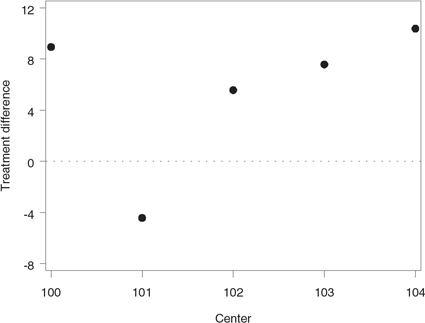
Output 1.1 lists the center-specific mean and standard deviation of the HAMD17 change scores in the two treatment groups. Further, Figure 1.1 displays the mean treatment differences observed at the five centers. Note that the mean treatment differences are fairly consistent at Centers 100, 102, 103 and 104. However, the data from Center 101 appears to be markedly different from the rest of the data.
As an aside note, it is helpful to remember that the likelihood of observing a similar treatment effect reversal by chance increases very quickly with the number of strata, and it is too early to conclude that Center 101 represents a true outlier (Senn, 1997, Chapter 14). We will discuss the problem of testing for qualitative treatment-by-stratum interactions in Section 1.5.
1.2.1 Fixed Effects Models
To introduce fixed effects models used in the analysis of stratified data, consider a study with a continuous endpoint comparing an experimental drug to a placebo across m strata (see Table 1.1). Suppose that the normally distributed outcome yijk observed on the kth patient in the jth stratum in the ith treatment group follows a two-way cell-means model
yijk=μij+εijk.(1.1)
In the depression trial example, the term yijk denotes the reduction in the HAMD17 score in individual patients and μij represents the mean reduction in the 10 cells defined by unique combinations of the treatment and stratum levels.
Table 1.1 A two-arm clinical trial with m strata
| Stratum 1 | Stratum m | |||||
| Treatment | Number of patients | Mean | ... | Treatment | Number of patients | Mean |
| Drug | n11 | μ11 | Drug | n1m | μ1m | |
| Placebo | n21 | μ21 | Placebo | n2m | μ2m | |
The cell-means model goes back to Scheffe (1959) and has been discussed in numerous publications, including Speed, Hocking and Hackney (1978) and Milliken and Johnson (1984). Let n1 j and n2j denote the sizes of the j th stratum in the experimental and placebo groups, respectively. Since it is uncommon to encounter empty strata in a clinical trial setting, we will assume there are no empty cells, i.e., nij > 0. Let n1 and n2 denote the number of patients in the experimental and placebo groups, and let n denote the total sample size, i.e.,
n1=m∑j=1n1j, n2=m∑j=1n2j, n=n1+n2.
A special case of the cell-means model (1.1) is the familiar main-effects model with an interaction
yijk=μ+αi+βj+(αβ)ij+εijk,(1.2)
where μ denotes the overall mean, the α parameters represent the treatment effects, the β parameters represent the stratum effects, and the αβ parameters are introduced to capture treatment-by-stratum variability.
Stratified data can be analyzed using several SAS procedures, including PROC ANOVA, PROC GLM and PROC MIXED. Since PROC ANOVA supports balanced designs only, we will focus in this section on the other two procedures. PROC GLM and PROC MIXED provide the user with several analysis options for testing the most important types of hypotheses about the treatment effect in the main-effects model (1.2). This section reviews hypotheses tested by the Type I, Type II and Type III analysis methods. The Type IV analysis will not be discussed here because it is different from the Type III analysis only in the rare case of empty cells. The reader can find more information about Type IV analyses in Milliken and Johnson (1984) and Littell, Freund and Spector (1991).
Type I Analysis
The Type I analysis is commonly introduced using the so-called R () notation proposed by Searle (1971, Chapter 6). Specifically, let R (μ) denote the reduction in the error sum of squares due to fitting the mean μ, i.e., fitting the reduced model
yijk=μ+εijk.
Similarly, R (μ, α) is the reduction in the error sum of squares associated with the model with the mean μ and treatment effect α, i.e.,
yijk=μ+αi+εijk.
The difference R(μ, α) – R(μ), denoted by R (α|μ), represents the additional reduction due to fitting the treatment effect after fitting the mean and helps assess the amount of variability explained by the treatment accounting for the mean μ. This notation is easy to extend to define other quantities such as R (β| μ, α). It is important to note that R (α|μ), R (β|μ, α) and other similar quantities are independent of restrictions imposed on parameters when they are computed from the normal equations. Therefore, R (α|μ), R (β|μ, α) and the like are uniquely defined in any two-way classification model.
The Type I analysis is based on testing the α, β and αβ factors in the main-effects model (1.2) in a sequential manner using R (α| μ), R (β|μ, α) and R (αβ|μ, α, β), respectively. Program 1.2 computes the F statistic and associated p-value for testing the difference between the experimental drug and placebo in the depression trial example.
Program 1.2 Type I analysis of the HAMD17 changes in the depression trial example
proc glm data=hamd17;
class drug center;
model change=drug|center/ss1;
run;
Output from Program 1.2
| Source | DF | Type I SS | Mean Square | F Value | Pr > F |
| drug | 1 | 888.0400000 | 888.0400000 | 40.07 | <.0001 |
| center | 4 | 87.1392433 | 21.7848108 | 0.98 | 0.4209 |
| drug*center | 4 | 507.4457539 | 126.8614385 | 5.72 | 0.0004 |
Output 1.2 lists the F statistics associated with the DRUG and CENTER effects as well as their interaction (recall that drug|center is equivalent to drug center drug*center). Since the Type I analysis depends on the order of terms, it is important to make sure that the DRUG term is fitted first. The F statistic for the treatment comparison, represented by the DRUG term, is very large (F = 40.07), which means that administration of the experimental drug results in a significant reduction of the HAMD17 score compared to the placebo. Note that this unadjusted analysis ignores the effect of centers on the outcome variable.
The R () notation helps clarify the structure and computational aspects of the inferences; however, as stressed by Speed and Hocking (1976), the notation may be confusing, and precise specification of the hypotheses being tested is clearly more helpful. As shown by Searle (1971, Chapter 7), the Type I F statistic for the treatment effect corresponds to the following hypothesis:
HI: 1n1m∑j=1n1jμ1j =1n2m∑j=1n2jμ2j.
It is clear that the Type I hypothesis of no treatment effect depends both on the true within-stratum means and the number of patients in each stratum.
Speed and Hocking (1980) presented an interesting characterization of the Type I, II and III analyses that facilitates the interpretation of the underlying hypotheses. Speed and Hocking showed that the Type I analysis tests the simple hypothesis of no treatment effect
H: 1mm∑j=1μ1j=1mm∑j=1μ2j
under the condition that the β and αβ factors are both equal to 0. This characterization implies that the Type I analysis ignores center effects and it is prudent to perform it when the stratum and treatment-by-stratum interaction terms are known to be negligible.
The standard ANOVA approach outlined above emphasizes hypothesis testing and it is helpful to supplement the computed p-value for the treatment comparison with an estimate of the average treatment difference and a 95% confidence interval. The estimation procedure is closely related to the Type I hypothesis of no treatment effect. Specifically, the “average treatment difference” is estimated in the Type I framework by
1n1m∑j=1n1jˉy1j.−1n2m∑j=1n2jˉy2j..
It is easy to verify from Output 1.1 and Model (1.2) that the Type I estimate of the average treatment difference in the depression trial example is equal to
ˆδ=^α1−^α2+(1150−1350)^β1+(750−750)^β2+(1650−1450)^β3+(950−1050)^β4+(750−650)^β5+1150(^αβ)11+750(^αβ)12+1650(^αβ)13+950(^αβ)14+750(^αβ)15−1350(^αβ)21−750(^αβ)22−1450(^αβ)23−1050(^αβ)24−650(^αβ)25=^α1−^α2−0.04^β1+0^β2+0.04^β3−0.02^β4+0.02^β5+0.22(^αβ)11+0.14(^αβ)12+0.32(^αβ)13+0.18(^αβ)14+0.14(^αβ)15−0.26(^αβ)21−0.14(^αβ)22−0.28(^αβ)23−0.2(^αβ)24−0.12(^αβ)25.
To compute this estimate and its associated standard error, we can use the ESTIMATE statement in PROC GLM as shown in Program 1.3.
Program 1.3 Type I estimate of the average treatment difference in the depression trial example
proc glm data=hamd17;
class drug center;
model change=drug|center/ss1;
estimate "Trt diff"
drug 1 -1
center -0.04 0 0.04 -0.02 0.02
drug*center 0.22 0.14 0.32 0.18 0.14 -0.26 -0.14 -0.28 -0.2 -0.12;
run;
Output from Program 1.3
| Parameter | Estimate | Standard Error | t Value | Pr > |t| |
| Trt diff | 5.96000000 | 0.94148228 | 6.33 | <.0001 |
Output 1.3 displays an estimate of the average treatment difference along with its standard error, which can be used to construct a 95% confidence interval associated with the obtained estimate. The t test for the equality of the treatment difference to 0 is identical to the F test for the DRUG term in Output 1.2. One can check that the t statistic in Output 1.3 is equal to the square root of the corresponding F statistic in Output 1.2. It is also easy to verify that the average treatment difference is simply the difference between the mean changes in the HAMD17 score observed in the experimental and placebo groups without any adjustment for center effects.
Type II Analysis
In the Type II analysis, each term in the main-effects model (1.2) is adjusted for all other terms with the exception of higher-order terms that contain the term in question. Using the R() notation, the significance of the α, β and αβ factors is tested in the Type II framework using R(α|μ, β), R(β|μ, α) and R(αβ|μ, α, β), respectively.
Program 1.4 computes the Type II F statistic to test the significance of the treatment effect on changes in the HAMD17 score.
Program 1.4 Type II analysis of the HAMD17 changes in the depression trial example
proc glm data=hamd17;
class drug center;
model change=drug|center/ss2;
run;
Output from Program 1.4
| Source | DF | Type II SS | Mean Square | F Value | Pr > F |
| drug | 1 | 889.7756912 | 889.7756912 | 40.15 | <.0001 |
| center | 4 | 87.1392433 | 21.7848108 | 0.98 | 0.4209 |
| drug*center | 4 | 507.4457539 | 126.8614385 | 5.72 | 0.0004 |
We see from Output 1.4 that the F statistic corresponding to the DRUG term is highly significant (F = 40.15), which indicates that the experimental drug significantly reduces the HAMD17 score after an adjustment for the center effect. Note that, by the definition of the Type II analysis, the presence of the interaction term in the model or the order in which the terms are included in the model do not affect the inferences with respect to the treatment effect. Thus, dropping the DRUG*CENTER term from the model generally has little impact on the F statistic for the treatment effect (to be precise, excluding the DRUG*CENTER term from the model has no effect on the numerator of the F statistic but affects its denominator due to the change in the error sum of squares).
Searle (1971, Chapter 7) demonstrated that the hypothesis of no treatment effect tested in the Type II framework has the following form:
HII: m∑j=1n1jn2jn1j+n2jμ1j=m∑j=1n1jn2jn1j+n2jμ2j.
Again, as in the case of Type I analyses, the Type II hypothesis of no treatment effect depends on the number of patients in each stratum. It is interesting to note that the variance of the estimated treatment difference in the j th stratum, i.e., Var (ȳ1j. – ȳ2j.), is inversely proportional to n1j n2 j/(n1 j + n2j). This means that the Type II method averages stratum-specific estimates of the treatment difference with weights proportional to the precision of the estimates.
The Type II estimate of the average treatment difference is given by
(m∑j=1n1jn2jn1j+n2j)−1 m∑j=1n1jn2jn1j+n2j(ˉy1j.−ˉy2j.).(1.3)
For example, we can see from Output 1.1 and Model (1.2) that the Type II estimate of the average treatment difference in the depression trial example equals
ˆδ=^α1−^α2+(11×1311+13+7×77+7+16×1416+14+9×10⁹+10+7×67+6)−1×(11×1311+13^(αβ)11+7×77+7^(αβ)12+16×1416+14^(αβ)13+9×10⁹+10^(αβ)14+7×67+6^(αβ)15−11×1311+13^(αβ)21−7×77+7^(αβ)22−16×1416+14^(αβ)23−9×10⁹+10^(αβ)24−7×67+6^(αβ)25)
=^α1−^α2+0.23936^(αβ)11+0.14060^(αβ)12+0.29996^(αβ)13+0.019029^(αβ)14+0.12979^(αβ)15−0.23936^(αβ)21−0.14060^(αβ)22−0.29996^(αβ)23−0.19029^(αβ)24−0.12979^(αβ)25.
Program 1.5 computes the Type II estimate and its standard error using the ESTIMATE statement in PROC GLM.
Program 1.5 Type II estimate of the average treatment difference in the depression trial example
proc glm data=hamd17;
class drug center;
model change=drug|center/ss2;
estimate "Trt diff"
drug 1 -1
drug*center 0.23936 0.14060 0.29996 0.19029 0.12979 -0.23936 -0.14060 -0.29996 -0.19029 -0.12979;
run;
Output from Program 1.5
| Parameter | Estimate | Standard Error | t Value | Pr > |t| | |
| Trt diff | 5.97871695 | 0.94351091 | 6.34 | <.0001 | |
Output 1.5 shows the Type II estimate of the average treatment difference and its standard error. As in the Type I framework, the t statistic in Output 1.5 equals the square root of the corresponding F statistic in Output 1.4, which implies that the two tests are equivalent. Note also that the t statistics for the treatment comparison produced by the Type I and II analysis methods are very close in magnitude, t = 6.33 in Output 1.3 and t = 6.34 in Output 1.5. This similarity is not a coincidence and is explained by the fact that patient randomization was stratified by center in this trial. As a consequence, n1j is close to n2j for any j = 1,…, 5 and thus n1j n2j /(n1j + n2j) is proportional to n1j. The weighting schemes underlying the Type I and II tests are almost identical to each other, which causes the two methods to yield similar results. Since the Type II method becomes virtually identical to the simple Type I method when patient randomization is stratified by the covariate used in the analysis, one does not gain much from using the randomization factor as a covariate in a Type II analysis. In general, however, the standard error of the Type II estimate of the treatment difference is considerably smaller than that of the Type I estimate and therefore the Type II method has more power to detect a treatment effect compared to the Type I method.
As demonstrated by Speed and Hocking (1980), the Type II method tests the simple hypothesis
H: 1mm∑j=1μ1j=1mm∑j=1μ2j
when the αβ factor is assumed to equal 0 (Speed and Hocking, 1980). In other words, the Type II analysis method arises naturally in trials where the treatment difference does not vary substantially from stratum to stratum.
Type III Analysis
The Type III analysis is based on a generalization of the concepts underlying the Type I and Type II analyses. Unlike these two analysis methods, the Type III methodology relies on a reparametrization of the main-effects model (1.2). The reparametrization is performed by imposing certain restrictions on the parameters in (1.2) in order to achieve a full-rank model. For example, it is common to assume that
2∑i=1αi=0,m∑j=1βj=0,2∑i=1(αβ)ij=0, j=1,...,m, m∑j=1(αβ)ij=0, i=1,2.(1.4)
Once the restrictions have been imposed, one can test the α, β and αβ factors using the R quantities associated with the obtained reparametrized model (these quantities are commonly denoted by R*).
The introduced analysis method is more flexible than the Type I and II analyses and allows one to test hypotheses that cannot be tested using the original R quantities (Searle, 1976; Speed and Hocking, 1976). For example, as shown by Searle (1971, Chapter 7), R(α|μ, β, αβ) and R(β|μ, α, αβ) are not meaningful when computed from the main-effects model (1.2) because they are identically equal to 0. This means that the Type I/II framework precludes one from fitting an interaction term before the main effects. By contrast, R*(α|μ, β, αβ) and R*(β|μ, α, αβ) associated with the full-rank reparametrized model can assume non-zero values depending on the constraints imposed on the model parameters. Thus, each term in (1.2) can be tested in the Type III framework using an adjustment for all other terms in the model.
The Type III analysis in PROC GLM and PROC MIXED assesses the significance of the α, β and αβ factors using R*(α|μ, β, αβ), R*(β|μ, α, αβ) and R*(αβ|μ, α, β) with the parameter restrictions given by (1.4). As an illustration, Program 1.6 tests the significance of the treatment effect on HAMD17 changes using the Type III approach.
Program 1.6 Type III analysis of the HAMD17 changes in the depression trial example
proc glm data=hamd17;
class drug center;
model change=drug|center/ss3;
run;
Output from Program 1.6
| Source | DF | Type III SS | Mean Square | F Value | Pr > F |
| drug | 1 | 709.8195519 | 709.8195519 | 32.03 | <.0001 |
| center | 4 | 91.4580063 | 22.8645016 | 1.03 | 0.3953 |
| drug*center | 4 | 507.4457539 | 126.8614385 | 5.72 | 0.0004 |
Output 1.6 indicates that the results of the Type III analysis are consistent with the Type I and II inferences for the treatment comparison. The treatment effect is highly significant after an adjustment for the center effect and treatment-by-center interaction (F = 32.03).
The advantage of making inferences from the reparametrized full-rank model is that the Type III hypothesis of no treatment effect has the following simple form (Speed, Hocking and Hackney, 1978):
HIII: 1mm∑j=1μ1j=1mm∑j=1μ2j.
The Type III hypothesis states that the simple average of the true stratum-specific HAMD17 change scores is identical in the two treatment groups. The corresponding Type III estimate of the average treatment difference is equal to
1mm∑j=1(ˉy1j.−ˉy2j.).
It is instructive to contrast this estimate with the Type I estimate of the average treatment difference. As was explained earlier, the idea behind the Type I approach is that individual observations are weighted equally. By contrast, the Type III method is based on weighting observations according to the size of each stratum. As a result, the Type III hypothesis involves a direct comparison of stratum means and is not affected by the number of patients in each individual stratum. To make an analogy, the Type I analysis corresponds to the U.S. House of Representatives, where the number of representatives from each state is a function of the state’s population. The Type III analysis can be thought of as a statistical equivalent of the U.S. Senate, where each state sends along two Senators.
Since the Type III estimate of the average treatment difference in the depression trial example is given by
ˆδ=^α1−^α2+15[^(αβ)11+^(αβ)12+^(αβ)13+^(αβ)14+^(αβ)15−^(αβ)21−^(αβ)22−^(αβ)23−^(αβ)24−^(αβ)25],
we can compute the estimate and its standard error using the following ESTIMATE statement in PROC GLM.
Program 1.7 Type III estimate of the average treatment difference in the depression trial example
proc glm data=hamd17;
class drug center;
model change=drug|center/ss3;
estimate "Trt diff"
drug 1 -1
drug*center 0.2 0.2 0.2 0.2 0.2 -0.2 -0.2 -0.2 -0.2 -0.2;
run;
Output from Program 1.7
| Parameter | Estimate | Standard Error | t Value | Pr > |t| | |
| Trt diff | 5.60912865 | 0.99106828 | 5.66 | <.0001 | |
Output 1.7 lists the Type III estimate of the treatment difference and its standard error. Again, the significance of the treatment effect can be assessed using the t statistic shown in Output 1.7 since the associated test is equivalent to the F test for the DRUG term in Output 1.6.
Comparison of Type I, Type II and Type III Analyses
The three analysis methods introduced in this section produce identical results in any balanced data set. The situation, however, becomes much more complicated and confusing in an unbalanced setting and one needs to carefully examine the available options to choose the most appropriate analysis method. The following comparison of the Type I, II and III analyses in PROC GLM and PROC MIXED will help the reader make more educated choices in clinical trial applications.
Type I Analysis
The Type I analysis method averages stratum-specific treatment differences with each observation receiving the same weight, and thus the Type I approach ignores the effects of individual strata on the outcome variable. It is clear that this approach can be used only if one is not interested in adjusting for the stratum effects.
Type II Analysis
The Type II approach amounts to comparing weighted averages of within-stratum estimates among the treatment groups. The weights are inversely proportional to the variances of stratum-specific estimates of the treatment effect, which implies that the Type II analysis is based on an optimal weighting scheme when there is no treatment-by-stratum interaction. When the treatment difference does vary across strata, the Type II test statistic can be viewed as a weighted average of stratum-specific treatment differences with the weights equal to sample estimates of certain population parameters. For this reason, it is commonly accepted that the Type II method is the preferred way of analyzing continuous outcome variables adjusted for prognostic factors (Fleiss, 1986; Mehrotra, 2001).
Attempts to apply the Type II method to stratification schemes based on nonprognostic factors (e.g., centers) have created much controversy in the clinical trial literature. Advocates of the Type II approach maintain that centers play the same role as prognostic factors, and thus it is appropriate to carry out Type II tests in trials stratified by center as shown in Program 1.4 (Senn, 1998; Lin, 1999). Note that the outcome of the Type II analysis is unaffected by the significance of the interaction term. The interaction analysis is run separately as part of routine sensitivity analyses such as the assessment of treatment effects in various subsets and the identification of outliers (Kallen, 1997; Phillips et al., 2000).
Type III Analysis
The opponents of the Type II approach argue that centers are intrinsically different from prognostic factors. Since investigative sites actively recruit patients, the number of patients enrolled at any given center is a rather arbitrary figure, and inferences driven by the sizes of individual centers are generally difficult to interpret (Fleiss, 1986). As an alternative, one can follow Yates (1934) and Cochran (1954a), who proposed to perform an analysis based on a simple average of center-specific estimates in the presence of a pronounced interaction. This unweighted analysis is equivalent to the Type III analysis of the model with an interaction term (see Program 1.6).
It is worth drawing the reader’s attention to the fact that the described alternative approach based on the Type III analysis has a number of limitations:
• The Type II F statistic is generally larger than the Type III F statistic (compare Output 1.4 and Output 1.6) and thus the Type III analysis is less powerful than the Type II analysis when the treatment difference does not vary much from center to center.
• The Type III method violates the marginality principle formulated by Nelder (1977). The principle states that meaningful inferences in a two-way classification setting are to be based on the main effects α and β adjusted for each other and on their interaction adjusted for the main effects. When one fits an interaction term before the main effects (as in the Type III analysis), the resulting test statistics depend on a totally arbitrary choice of parameter constraints. The marginality principle implies that the Type III inferences yield uninterpretable results in unbalanced cases. See Nelder (1994) and Rodriguez, Tobias and Wolfinger (1995) for a further discussion of pros and cons of this argument.
• Weighting small and large strata equally is completely different from how one would normally perform a meta-analysis of the results observed in the strata (Senn, 2000).
• Lastly, as pointed out in several publications, sample size calculations are almost always done within the Type II framework; i.e., patients rather than centers are assumed equally weighted. As a consequence, the use of the Type III analysis invalidates the sample size calculation method. For a detailed power comparison of the weighted and unweighted approaches, see Jones et al. (1998) and Gallo (2000).
Type III Analysis with Pretesting
The described weighted and unweighted analysis methods are often combined to increase the power of the treatment comparison. As proposed by Fleiss (1986), the significance of the interaction term is assessed first and the Type III analysis with an interaction is performed if the preliminary test has yielded a significant outcome. Otherwise, the interaction term is removed from the model and thus the treatment effect is analyzed using the Type II approach. The sequential testing procedure recognizes the power advantage of the weighted analysis when the treatment-by-center interaction appears to be negligible.
Most commonly, the treatment-by-center variation is evaluated using an F test based on the interaction mean square; see the F test for the DRUG*CENTER term in Output 1.6. This test is typically carried out at the 0.1 significance level (Fleiss, 1986). Several alternative approaches have been suggested in the literature. Bancroft (1968) proposed to test the interaction term at the 0.25 level before including it in the model. Chinchilli and Bortey (1991) described a test for consistency of treatment differences across strata based on the noncentrality parameter of an F distribution. Ciminera et al. (1993) stressed that tests based on the interaction mean square are aimed at detecting quantitative interactions that may be caused by a variety of factors such as measurement scale artifacts. To alleviate the problems associated with the traditional pretesting approach, Ciminera et al. outlined an alternative method that relies on qualitative interactions ; see Section 1.5 for more details.
When applying the pretesting strategy, one needs to be aware of the fact that pretesting leads to more frequent false-positive outcomes, which may become an issue in pivotal clinical trials. To stress this point, Jones et al. (1998) compared the described pretesting approach with the controversial practice of pretesting the significance of the carryover effect in crossover trials, a practice that is known to inflate the false-positive rate.
1.2.2 Random Effects Models
A popular alternative to the fixed effects modeling approach described in Section 1.2.1 is to explicitly incorporate random variation among strata in the analysis. Even though most of the discussion on center effects in the ICH guidance document “Statistical principles for clinical trials” (ICH E9) treats center as a fixed effect, the guidance also encourages trialists to explore the heterogeneity of the treatment effect across centers using mixed models. The latter can be accomplished by employing models with random stratum and treatment-by-stratum interaction terms. While one can argue that the selection of centers is not necessarily a random process, treating centers as a random effect could at times help statisticians better account for between-center variability.
Random effects modeling is based on the following mixed model for the continuous outcome yijk observed on the kth patient in the jth stratum in the ith treatment group:
yijk=μ+αi+bj+gij+εijk,(1.5)
where μ denotes the overall mean, αi is the fixed effect of the ith treatment, bj and gij denote the random stratum and treatment-by-stratum interaction effects, and εijk is a residual term. The random and residual terms are assumed to be normally distributed and independent of each other. We can see from Model (1.5) that, unlike fixed effects models, random effects models account for the variability across strata in judging the significance of the treatment effect.
Applications of mixed effects models to stratified analyses in a clinical trial context were described by several authors, including Fleiss (1986), Senn (1998) and Gallo (2000). Chakravorti and Grizzle (1975) provided a theoretical foundation for random effects modeling in stratified trials based on the familiar randomized block design framework and the work of Hartley and Rao (1967). For a detailed overview of issues related to the analysis of mixed effects models, see Searle (1992, Chapter 3). Littell et al. (1996, Chapter 2) demonstrated how to use PROC MIXED in order to fit random effects models in multicenter trials.
Program 1.8 fits a random effects model to the HAMD17 data set using PROC MIXED and computes an estimate of the average treatment difference. The DDFM=SATTERTH option in Program 1.8 requests that the degrees of freedom for the F test be computed using the Satterthwaite formula. The Satterthwaite method provides a more accurate approximation to the distribution of the F statistic in random effects models than the standard ANOVA method (it is achieved by increasing the number of degrees of freedom for the F statistic).
Program 1.8 Analysis of the HAMD17 changes in the depression trial example using a random effects model
proc mixed data=hamd17;
class drug center;
model change=drug/ddfm=satterth;
random center drug*center;
estimate "Trt eff" drug 1 -1;
run;
Output from Program 1.8
| Type 3 Tests of Fixed Effects | |||||
| Effect | Num DF |
Den DF |
F Value | Pr > F | |
| drug | 1 | 6.77 | 9.30 | 0.0194 | |
| Estimates | |||||
| Label | Estimate | Standard Error |
DF | t Value | Pr > |t| |
| Trt eff | 5.7072 | 1.8718 | 6.77 | 3.05 | 0.0194 |
Output 1.8 displays the F statistic (F = 9.30) and p-value (p = 0.0194) associated with the DRUG term in the random effects model as well as an estimate of the average treatment difference. The estimated treatment difference equals 5.7072 and is close to the estimates computed from fixed effects models. The standard error of the estimate (1.8718) is substantially greater than the standard error of the estimates obtained in fixed effects models (see Output 1.6). This is a penalty one has to pay for treating the stratum and interaction effects as random, and it reflects lack of homogeneity across the five strata in the depression data. Note, for example, that dropping Center 101 creates more homogeneous strata and, as a consequence, reduces the standard error to 1.0442. Similarly, removing the DRUG*CENTER term from the RANDOM statement leads to a more precise estimate of the treatment effect with the standard error of 1.0280.
In general, as shown by Senn (2000), fitting main effects as random leads to lower standard errors; however, assuming a random interaction term increases the standard error of the estimated treatment difference. Due to the lower precision of treatment effect estimates, analysis of stratified data based on models with random stratum and treatment-by-stratum effects has lower power compared to a fixed effects analysis (Gould, 1998; Jones et al., 1998).
1.2.3 Nonparametric Tests
This section briefly describes a nonparametric test for stratified continuous data proposed by van Elteren (1960). To introduce the van Elteren test, consider a clinical trial with a continuous endpoint measured in m strata. Let w j denote the Wilcoxon rank-sum statistic for testing the null hypothesis of no treatment effect in the jth stratum (Hollander and Wolfe, 1999, Chapter 4). Van Elteren (1960) proposed to combine stratum-specific Wilcoxon rank-sum statistics with weights inversely proportional to stratum sizes. The van Elteren statistic is given by
u=m∑j=1wjn1j+n2j+1,
where n1j + n2j is the total number of patients in the jth stratum. To justify this weighting scheme, van Elteren demonstrated that the resulting test has asymptotically the maximum power against a broad range of alternative hypotheses. Van Elteren also studied the asymptotic properties of the testing procedure and showed that, under the null hypothesis of no treatment effect in the m strata, the test statistic is asymptotically normal.
As shown by Koch et al. (1982, Section 2.3), the van Elteren test is a member of a general family of Mantel-Haenszel mean score tests. This family also includes the Cochran-Mantel-Haenszel test for categorical outcomes discussed later in Section 1.3.1. Like other testing procedures in this family, the van Elteren test possesses an interesting and useful property that its asymptotic distribution is not directly affected by the size of individual strata. As a consequence, one can rely on asymptotic p-values even in sparse stratifications as long as the total sample size is large enough. For more information about the van Elteren test and related testing procedures, see Lehmann (1975), Koch et al. (1990) and Hosmane, Shu and Morris (1994).
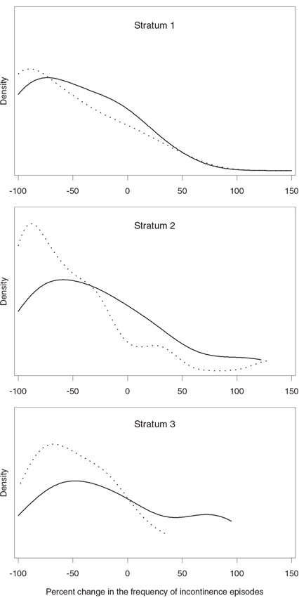
EXAMPLE: Urinary Incontinence Trial
The van Elteren test is an alternative method of analyzing stratified continuous data when one cannot rely on standard ANOVA techniques because the underlying normality assumption is not met. As an illustration, consider a subset of the data collected in a urinary incontinence trial comparing an experimental drug to a placebo over an 8-week period. The primary endpoint in the trial was a percent change from baseline to the end of the study in the number of incontinence episodes per week. Patients were allocated to three strata according to the baseline frequency of incontinence episodes.2
Program 1.9 displays a subset of the data collected in the urinary incontinence trial and plots the probability distribution of the primary endpoint in the three strata.
Program 1.9 Distribution of percent changes in the frequency of incontinence episodes in the urinary incontinence trial example
data urininc;
input therapy $ stratum @@;
do i=1 to 10;
input change @@;
if (change^=.) then output;
end;
drop i;
datalines;
| Placebo | 1 | -86 | -38 | 43 | -100 | 289 | 0 | -78 | 38 | -80 | -25 |
| Placebo | 1 | -100 | -100 | -50 | 25 | -100 | -100 | -67 | 0 | 400 | -100 |
| Placebo | 1 | -63 | -70 | -83 | -67 | -33 | 0 | -13 | -100 | 0 | -3 |
| Placebo | 1 | -62 | -29 | -50 | -100 | 0 | -100 | -60 | -40 | -44 | -14 |
| Placebo | 2 | -36 | -77 | -6 | -85 | 29 | -17 | -53 | 18 | -62 | -93 |
| Placebo | 2 | 64 | -29 | 100 | 31 | -6 | -100 | -30 | 11 | -52 | -55 |
| Placebo | 2 | -100 | -82 | -85 | -36 | -75 | -8 | -75 | -42 | 122 | -30 |
| Placebo | 2 | 22 | -82 | . | . | . | . | . | . | . | . |
| Placebo | 3 | 12 | -68 | -100 | 95 | -43 | -17 | -87 | -66 | -8 | 64 |
| Placebo | 3 | 61 | -41 | -73 | -42 | -32 | 12 | -69 | 81 | 0 | 87 |
| Drug | 1 | 50 | -100 | -80 | -57 | -44 | 340 | -100 | -100 | -25 | -74 |
| Drug | 1 | 0 | 43 | -100 | -100 | -100 | -100 | -63 | -100 | -100 | -100 |
| Drug | 1 | -100 | -100 | 0 | -100 | -50 | 0 | 0 | -83 | 369 | -50 |
| Drug | 1 | -33 | -50 | -33 | -67 | 25 | 390 | -50 | 0 | -100 | . |
| Drug | 2 | -93 | -55 | -73 | -25 | 31 | 8 | -92 | -91 | -89 | -67 |
| Drug | 2 | -25 | -61 | -47 | -75 | -94 | -100 | -69 | -92 | -100 | -35 |
| Drug | 2 | -100 | -82 | -31 | -29 | -100 | -14 | -55 | 31 | -40 | -100 |
| Drug | 2 | -82 | 131 | -60 | . | . | . | . | . | . | . |
| Drug | 3 | -17 | -13 | -55 | -85 | -68 | -87 | -42 | 36 | -44 | -98 |
| Drug | 3 | -75 | -35 | 7 | -57 | -92 | -78 | -69 | -21 | -14 | . |
| ; | |||||||||||
proc sort data=urininc;
by stratum therapy;
proc kde data=urininc out=density;
by stratum therapy;
var change;
proc sort data=density;
by stratum;
* Plot the distribution of the primary endpoint in each stratum;
%macro PlotDist(stratum,label);
axis1 minor=none major=none value=none label=(angle=90 "Density")
order=(0 to 0.012 by 0.002);
axis2 minor=none order=(-100 to 150 by 50)
label=("&label");
symbol1 value=none color=black i=join line=34;
symbol2 value=none color=black i=join line=1;
data annotate;
xsys="1"; ysys="1"; hsys="4"; x=50; y=90; position="5";
size=1; text="Stratum &stratum"; function="label";
proc gplot data=density anno=annotate;
where stratum=&stratum;
plot density*change=therapy/frame haxis=axis2 vaxis=axis1 nolegend;
run;
quit;
%mend PlotDist;
%PlotDist(1,);
%PlotDist(2,);
%PlotDist(3,Percent change in the frequency of incontinence episodes);
The output of Program 1.9 is shown in Figure 1.2. We can see from Figure 1.2 that the distribution of the primary outcome variable is consistently skewed to the right across the three strata. Since the normality assumption is clearly violated in this data set, the analysis methods described earlier in this section may perform poorly. The magnitude of treatment effect on the frequency of incontinence episodes can be assessed more reliably using a nonparametric procedure. Program 1.10 computes the van Elteren statistic to test the null hypothesis of no treatment effect in the urinary incontinence trial using PROC FREQ. The statistic is requested by including the CMH2 and SCORES=MODRIDIT options in the TABLE statement.
Program 1.10 Analysis of percent changes in the frequency of incontinence episodes using the van Elteren test
proc freq data=urininc;
ods select cmh;
table stratum*therapy*change/cmh2 scores=modridit;
run;
Output from Program 1.10
Summary Statistics for therapy by change
Controlling for stratum
Cochran-Mantel-Haenszel Statistics (Modified Ridit Scores)
| Statistic | Alternative Hypothesis | DF | Value | Prob |
| 1 | Nonzero Correlation | 1 | 6.2505 | 0.0124 |
| 2 | Row Mean Scores Differ | 1 | 6.2766 | 0.0122 |
Figure 1.2 The distribution of percent changes in the frequency of incontinence episodes in the experimental (…) and placebo (—) groups by stratum in the urinary incontinence trial
Output 1.10 lists two statistics produced by PROC FREQ (note that extraneous information has been deleted from the output using the ODS statement). The van Elteren statistic corresponds to the row mean scores statistic labeled “Row Mean Scores Differ” and is equal to 6.2766. Since the asymptotic p-value is small (p = 0.0122), we conclude that administration of the experimental drug resulted in a significant reduction in the frequency of incontinence episodes. To compare the van Elteren test with the Type II and III analyses in the parametric ANOVA framework, Programs 1.4 and 1.6 were rerun to test the significance of the treatment effect in the urinary incontinence trial. The Type II and III F statistics were equal to 1.4 (p = 0.2384) and 2.15 (p = 0.1446), respectively. The parametric methods were unable to detect the treatment effect in this data set due to the highly skewed distribution of the primary endpoint.
1.2.4 Summary
This section discussed parametric and nonparametric methods for performing stratified analyses in clinical trials with a continuous endpoint. Parametric analysis methods based on fixed and random effects models are easy to implement using PROC GLM (fixed effects only) or PROC MIXED (both fixed and random effects).
PROC GLM and PROC MIXED support three popular methods of fitting fixed effects models to stratified data. These analysis methods, known as Type I, II and III analyses, are conceptually similar to each other in the sense that they are all based on averaging stratum-specific estimates of the treatment effect. The following is a quick summary of the Type I, II and III methods:
• Each observation receives the same weight when a Type I average of stratum-specific treatment differences is computed. Therefore, the Type I approach ignores the effects of individual strata on the outcome variable.
• The Type II approach is based on a comparison of weighted averages of stratum-specific estimates of the treatment effect, with the weights being inversely proportional to the variances of these estimates. The Type II weighting scheme is optimal when there is no treatment-by-stratum interaction and can also be used when treatment differences vary across strata. It is generally agreed that the Type II method is the preferred way of analyzing continuous outcome variables adjusted for prognostic factors.
• The Type III analysis method relies on a direct comparison of stratum means, which implies that individual observations are weighted according to the size of each stratum. This analysis is typically performed in the presence of a significant treatment-by-stratum interaction. It is important to remember that Type II tests are known to have more power than Type III tests when the treatment difference does not vary much from stratum to stratum.
The information about treatment differences across strata can also be combined using random effects models in which stratum and treatment-by-stratum interaction terms are treated as random variables. Random effects inferences for stratified data can be implemented using PROC MIXED. The advantage of random effects modeling is that it helps the statistician better account for between-stratum variability. However, random effects inferences are generally less powerful than inferences based on fixed effects models. This is one of the reasons why stratified analyses based on random effects models are rarely performed in a clinical trial setting.
A stratified version of the nonparametric Wilcoxon rank-sum test, known as the van Elteren test, can be used to perform inferences in a non-normal setting. It has been shown that the asymptotic distribution of the van Elteren test statistic is not directly affected by the size of individual strata and therefore this testing procedure performs well in the analysis of a large number of small strata.
1.3 Categorical Endpoints
This section covers analysis of stratified categorical data in clinical trials. It discusses both asymptotic and exact approaches, including
• randomization-based Cochran-Mantel-Haenszel approach
• minimum variance methods
• model-based inferences.
Although the examples in this section deal with the case of binary outcomes, the described analysis methods can be easily extended to a more general case of multinomial variables. SAS procedures used below automatically invoke general categorical tests when the analysis variable assumes more than two values.
Also, the section reviews methods that treat stratification factors as fixed variables. It does not cover stratified analyses based on random effects models for categorical data because they are fairly uncommon in clinical applications. For a review of tests for stratified categorical data arising within a random effects modeling framework, see Lachin (2000, Section 4.10) and Agresti and Hartzel (2000).
Measures of Association
There are three common measures of association used with categorical data: risk difference, relative risk and odds ratio. To introduce these measures, consider a clinical trial designed to compare the effects of an experimental drug and a placebo on the incidence of a binary event such as improvement or survival in m strata (see Table 1.2). Let n1j1 and n2j1 denote the numbers of jth stratum patients in the experimental and placebo groups, respectively, who experienced an event of interest. Similarly, n1j2 and n2j2 denote the numbers of jth stratum patients in the experimental and placebo groups, respectively, who did not experience an event of interest.
Table 1.2 A two-arm clinical trial with m strata
| Stratum 1 | Stratum m | |||||||
| Treatment | Event | No event | Total | Treatment | Event | No event | Total | |
| Drug | n111 | n112 | n11+ | … | Drug | n1m1 | n1m2 | n1m+ |
| Placebo | n211 | n212 | n21+ | Placebo | n2m1 | n2m2 | n2m+ | |
| Total | n+11 | n+12 | n1 | Total | n+m1 | n+m2 | nm | |
The risk difference, relative risk and odds ratio of observing the binary event of interest are defined as follows:
• Risk difference. The true event rate in jth stratum is denoted by π1j in the experimental group and π2j in the placebo group and thus the risk difference equals di = π1j — π2j. The true event rates are estimated by sample proportions p1j = n1j1/n1j+ and p2j = n2j1/n2j+, and the risk difference is estimated by ^dj=p1j−p2j.
• Relative risk. The relative risk of observing the event in the experimental group compared to the placebo group is equal to rj = π1 j/π2 j in the jth stratum. This relative risk is estimated by ^rj=p1j/p2j. (assuming that p2 j> 0).
• Odds ratio. The odds of observing the event of interest in the jth stratum is π1 j/(1 – π1 j) in the experimental group and π2 j/(1 – π2 j) in the placebo group. The corresponding odds ratio in the jth stratum equals
oj=π1j1−π1j/π2j1−π2j
and is estimated by
^oj=p1j1−p1j/p2j1−p2j.
We assume here that p1 j < 1 and p2 j > 0.
Since the results and their interpretation may be affected by the measure of association used in the analysis, it is important to clearly specify whether the inferences are based on risk differences, relative risks or odds ratios.
EXAMPLE: Severe Sepsis Trial
Statistical methods for the analysis of stratified clinical trials with a binary endpoint will be illustrated using the following data. A placebo-controlled clinical trial was conducted on 1690 patients to examine the effect of an experimental drug on 28-day all-cause mortality in patients with severe sepsis. Patients were assigned to one of four strata at randomization, depending on the predicted risk of mortality computed from the APACHE II score (Knaus et al., 1985). The APACHE II score ranges from 0 to 71 and an increased score is correlated with a higher risk of death. The results observed in each of the four strata are summarized in Table 1.3.3
Table 1.3 28-day mortality data from a 1690-patient trial in patients with severe sepsis
| Stratum | Experimental drug | Placebo | |||||
| Dead | Alive | Total | Dead | Alive | Total | ||
| 1 | 33 | 185 | 218 | 26 | 189 | 215 | |
| 2 | 49 | 169 | 218 | 57 | 165 | 222 | |
| 3 | 48 | 156 | 204 | 58 | 104 | 162 | |
| 4 | 80 | 130 | 210 | 118 | 123 | 241 | |
Programs 1.11 and 1.12 below summarize the survival and mortality data collected in the sepsis trial. Program 1.11 uses PROC FREQ to compute the risk difference, relative risk and odds ratio of mortality in patients at a high risk of death (Stratum 4).
Program 1.11 Summary of survival and mortality data in the severe sepsis trial example (Stratum 4)
data sepsis;
input stratum therapy $ outcome $ count @@;
if outcome="Dead" then survival=0; else survival=1;
datalines;
| 1 | Placebo | Alive | 189 | 1 | Placebo | Dead | 26 |
| 1 | Drug | Alive | 185 | 1 | Drug | Dead | 33 |
| 2 | Placebo | Alive | 165 | 2 | Placebo | Dead | 57 |
| 2 | Drug | Alive | 169 | 2 | Drug | Dead | 49 |
| 3 | Placebo | Alive | 104 | 3 | Placebo | Dead | 58 |
| 3 | Drug | Alive | 156 | 3 | Drug | Dead | 48 |
| 4 | Placebo | Alive | 123 | 4 | Placebo | Dead | 118 |
| 4 | Drug | Alive | 130 | 4 | Drug | Dead | 80 |
| ; | |||||||
proc freq data=sepsis;
where stratum=4;
table therapy*survival/riskdiff relrisk;
weight count;
run;
Output from Program 1.11
Column 1 Risk Estimates
| Risk | ASE | (Asymptotic) 95% Confidence Limits |
||
| Row 1 | 0.3810 | 0.0335 | 0.3153 | 0.4466 |
| Row 2 | 0.4896 | 0.0322 | 0.4265 | 0.5527 |
| Total | 0.4390 | 0.0234 | 0.3932 | 0.4848 |
| Difference | -0.1087 | 0.0465 | -0.1998 | -0.0176 |
Difference is (Row 1 - Row 2)
| (Exact) Confidence |
95% Limits |
|
| Row 1 | 0.3150 | 0.4503 |
| Row 2 | 0.4249 | 0.5546 |
| Total | 0.3926 | 0.4862 |
Difference is (Row 1 - Row 2)
Column 2 Risk Estimates
| Risk | ASE | (Asymptotic) Confidence | 95% Limits | |
| Row 1 | 0.6190 | 0.0335 | 0.5534 | 0.6847 |
| Row 2 | 0.5104 | 0.0322 | 0.4473 | 0.5735 |
| Total | 0.5610 | 0.0234 | 0.5152 | 0.6068 |
| Difference | 0.1087 | 0.0465 | 0.0176 | 0.1998 |
Difference is (Row 1 - Row 2)
| (Exact) Confidence |
95% Limits |
|
| Row 1 | 0.5497 | 0.6850 |
| Row 2 | 0.4454 | 0.5751 |
| Total | 0.5138 | 0.6074 |
Difference is (Row 1 - Row 2)
Estimates of the Relative Risk (Row1/Row2)
| Type of Study | Value | 95% Confidence | Limits |
| Case-Control (Odds Ratio) | 0.6415 | 0.4404 | 0.9342 |
| Cohort (Col1 Risk) | 0.7780 | 0.6274 | 0.9649 |
| Cohort (Col2 Risk) | 1.2129 | 1.0306 | 1.4276 |
Risk statistics shown under “Column 1 Risk Estimates” in Output 1.11 represent estimated 28-day mortality rates in the experimental (Row 1) and placebo (Row 2) groups. Similarly, risk statistics under “Column 2 Risk Estimates” refer to survival rates in the two treatment groups. PROC FREQ computes both asymptotic and exact confidence intervals for the estimated rates. The estimated risk difference is – 0.1087 and thus, among patients with a poor prognosis, patients treated with the experimental drug are 11% more likely to survive (in absolute terms) than those who received the placebo. Note that exact confidence intervals for risk differences are quite difficult to construct (see Coe and Tamhane (1993) for more details) and there is no exact confidence interval associated with the computed risk difference in survival or mortality rates.
Estimates of the ratio of the odds of mortality and relative risks of survival and mortality are given under “Estimates of the Relative Risk (Row1/Row2).” The odds ratio equals 0.6415, which indicates that the odds of mortality are 36% lower in the experimental group compared to the placebo group in the chosen subpopulation of patients. The corresponding relative risks of survival and mortality are 1.2129 and 0.7780, respectively. The displayed 95% confidence limits are based on a normal approximation. An exact confidence interval for the odds ratio can be requested using the EXACT statement with the OR option. PROC FREQ does not currently compute exact confidence limits for relative risks.
Program 1.12 demonstrates how to use the Output Delivery System (ODS) with PROC FREQ to compute risk differences, relative risks and odds ratios of mortality in all four strata.
Program 1.12 Summary of mortality data in the severe sepsis trial example (all strata)
proc freq data=sepsis noprint;
by stratum;
table therapy*survival/riskdiff relrisk;
ods output riskdiffcol1=riskdiff relativerisks=relrisk;
weight count;
* Plot of mortality rates;
data mortrate;
set riskdiff;
format risk 3.1;
if row="Row 1" then therapy="D";
if row="Row 2" then therapy="P";
if therapy="" then delete;
axis1 minor=none label=(angle=90 "Mortality rate") order=(0 to 0.6 by 0.2);
axis2 label=none;
pattern1 value=empty color=black;
pattern2 value=r1 color=black;
proc gchart data=mortrate;
vbar therapy/frame raxis=axis1 maxis=axis2 gaxis=axis2
sumvar=risk subgroup=therapy group=stratum nolegend;
run;
* Plot of risk differences;
data mortdiff;
set riskdiff;
format risk 4.1;
if row="Difference";
axis1 minor=none label=(angle=90 "Risk difference")
order=(-0.2 to 0.1 by 0.1);
axis2 label=("Stratum");
pattern1 value=empty color=black;
proc gchart data=mortdiff;
vbar stratum/frame raxis=axis1 maxis=axis2 sumvar=risk
midpoints=1 2 3 4;
run;
* Plot of relative risks;
data riskratio;
set relrisk;
format value 3.1;
if studytype="Cohort (Col1 Risk)";
axis1 minor=none label=(angle=90 "Relative risk")
order=(0.5 to 1.3 by 0.1);
axis2 label=("Stratum");
pattern1 value=empty color=black;
proc gchart data=riskratio;
vbar stratum/frame raxis=axis1 maxis=axis2 sumvar=value
midpoints=1 2 3 4;
run;
* Plot of odds ratios;
data oddsratio;
set relrisk;
format value 3.1;
if studytype="Case-Control (Odds Ratio)";
axis1 label=(angle=90 "Odds ratio") order=(0.4 to 1.4 by 0.2);
axis2 label=("Stratum");
pattern1 value=empty color=black;
proc gchart data=oddsratio;
vbar stratum/frame raxis=axis1 maxis=axis2 sumvar=value
midpoints=1 2 3 4;
run;
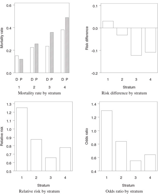
The output of Program 1.12 is displayed in Figure 1.3. Figure 1.3 shows that there was significant variability among the four strata in terms of 28-day mortality rates. The absolute reduction in mortality in the experimental group compared to the placebo group varied from —3.04% in Stratum 1 to 12.27% in Stratum 3. The treatment effect was most pronounced in patients with a poor prognosis at study entry (i.e., patients in Strata 3 and 4).
1.3.1 Asymptotic Randomization-Based Tests
Fleiss (1981, Chapter 10) described a general method for performing stratified analyses that goes back to Cochran (1954a) and applied it to the case of binary outcomes. Let aj denote the estimate of a certain measure of association between the treatment and binary outcome in the jth stratum, and let s2j be the sample variance of this estimate. Assume that the measure of association is chosen in such a way that it equals 0 when the treatment difference is 0. Also, wj will denote the reciprocal of the sample variance, i.e., wj=1/s2j. The total chi-square statistic
χ2T=m∑j=1wja2j
can be partitioned into a chi-square statistic χ2H for testing the degree of homogeneity among the strata and a chi-square statistic χ2A for testing the significance of overall association across the strata given by
χ2H=m∑j=1wj(aj−ˆa)2,(1.6)χ2A=(m∑j=1wj)−1(m∑j=1wjaj)2,(1.7)
Figure 1.3 A summary of mortality data in the severe sepsis trial example accompanied by three measures of treatment effect (D = Drug, P = Placebo)
where
ˆa=(m∑j=1wj)−1m∑j=1wjaj(1.8)
is the associated minimum variance estimate of the degree of association averaged across the m strata. Under the null hypothesis of homogeneous association, χ2H asymptotically follows a chi-square distribution with m – 1 degrees of freedom. Similarly, under the null hypothesis that the average association between the treatment and binary outcome is zero, χ2A is asymptotically distributed as chi-square with 1 degree of freedom.
The described method for testing hypotheses of homogeneity and association in a stratified setting can be used to construct a large number of useful tests. For example, if aj is equal to a standardized treatment difference in the jth stratum,
aj=^djˉpj(1−ˉpj), where¯ pj=n+j1/nj and ^dj=p1j−p2j,(1.9)
then
wj=ˉpj(1−ˉpj)n1j+n2j+n1j++n2j+.
The associated chi-square test of overall association based on χ2A is equivalent to a test for stratified binary data proposed by Cochran (1954b) and is asymptotically equivalent to a test developed by Mantel and Haenszel (1959). Due to their similarity, it is common to refer to the two tests collectively as the Cochran-Mantel-Haenszel (CMH) procedure. Since aj in (1.9) involves the estimated risk difference ^dj, the CMH procedure tests the degree of association with respect to the risk differences d1,…, dm in the m strata. The estimate of the average risk difference corresponding to the CMH test is given by
ˆd=(m∑j=1ˉpj(1−ˉpj)n1j+n2j+n1j++n2j+)−1m∑j=1n1j+n2j+n1j++n2j+^dj.(1.10)
It is interesting to compare this estimate to the Type II estimate of the average treatment effect in the continuous case (see Section 1.2.1). The stratum-specific treatment differences ^d1,…,^dm, are averaged in the CMH estimate with the same weights as in the Type II estimate and thus one can think of the CMH procedure as an extension of the Type II testing method to trials with a binary outcome. Although unweighted estimates corresponding to the Type III method have been mentioned in the literature, they are rarely used in the analysis of stratified trials with a categorical outcome and are not implemented in SAS.
One can use the general method described by Fleiss (1981, Chapter 10) to construct estimates and associated tests for overall treatment effect based on relative risks and odds ratios. Relative risks and odds ratios need to be transformed before the method is applied because they are equal to 1 in the absence of treatment effect. Most commonly, a log transformation is used to ensure that aj = 0, j = 1,…, m, when the stratum-specific treatment differences are equal to 0.
The minimum variance estimates of the average log relative risk and log odds ratio are based on the formula (1.8) with
aj=log^rj, wj=[(1n1j1−1n1j+)+(1n2j1−1n2j+)]−1 (log relative risk),(1.11)
aj=log^oj, wj=(1n1j1+1n1j2+1n2j1+1n2j2)−1 (log odds ratio).(1.12)
The corresponding estimates of the average relative risk and odds ratio, are computed using exponentiation. Adopting the PROC FREQ terminology, we will refer to these estimates as logit-adjusted estimates and denote them by ˆrL and ˆoL
It is instructive to compare the logit-adjusted estimates ˆrL and ˆoL with estimates of the average relative risk and odds ratio proposed by Mantel and Haenszel (1959). The Mantel-Haenszel estimates, denoted by ˆrMH and ˆoMH, can also be expressed as weighted averages of stratum-specific relative risks and odds ratios:
ˆrMH=(m∑j=1wj)−1m∑j=1wjˆrj, where wj=n2j1n1j+nj,
ˆoMH=(m∑j=1wj)−1m∑j=1wjˆoj, where wj=n2j1n1j2nj.
Note that weights in ˆrMH and ˆoMH are not inversely proportional to sample variances of the stratum-specific estimates and thus ˆrMH and ˆoMH do not represent minimum variance estimates. Despite this property, the Mantel-Haenszel estimates are generally comparable to the logit-adjusted estimates ˆrL and ˆoL in terms of precision. Also, as shown by Breslow (1981), ˆrMH and ˆoMH are attractive in applications because their mean square error is always less than that of the logit-adjusted estimates ˆrL and ˆoL. Further, Breslow (1981) and Greenland and Robins (1985) studied the asymptotic behavior of the Mantel-Haenszel estimates and demonstrated that, unlike the logit-adjusted estimates, they perform well in sparse stratifications.
The introduced estimates of the average risk difference, relative risk and odds ratio, as well as associated test statistics, are easy to obtain using PROC FREQ. Program 1.13 carries out the CMH test in the severe sepsis trial controlling for the baseline risk of mortality represented by the STRATUM variable. The program also computes the logit-adjusted and Mantel-Haenszel estimates of the average relative risk and odds ratio. Note that the order of the variables in the TABLE statement is very important; the stratification factor is followed by the other two variables.
Program 1.13 Average association between treatment and survival in the severe sepsis trial example
proc freq data=sepsis;
table stratum*therapy*survival/cmh;
weight count;
run;
Output from Program 1.13
Summary Statistics for therapy by outcome
Controlling for stratum
Cochran-Mantel-Haenszel Statistics (Based on Table Scores)
| Statistic | Alternative Hypothesis | DF | Value | Prob |
| 1 | Nonzero Correlation | 1 | 6.9677 | 0.0083 |
| 2 | Row Mean Scores Differ | 1 | 6.9677 | 0.0083 |
| 3 | General Association | 1 | 6.9677 | 0.0083 |
Estimates of the Common Relative Risk (Row1/Row2)
| Type of Study | Method | Value |
| Case-Control | Mantel-Haenszel | 0.7438 |
| (Odds Ratio) | Logit | 0.7426 |
| Cohort | Mantel-Haenszel | 0.8173 |
| (Col1 Risk) | Logit | 0.8049 |
| Cohort | Mantel-Haenszel | 1.0804 |
| (Col2 Risk) | Logit | 1.0397 |
| Type of Study | Method | 95% Confidence | Limits |
| Case-Control | Mantel-Haenszel | 0.5968 | 0.9272 |
| (Odds Ratio) | Logit | 0.5950 | 0.9267 |
| Cohort | Mantel-Haenszel | 0.7030 | 0.9501 |
| (Col1 Risk) | Logit | 0.6930 | 0.9349 |
| Cohort | Mantel-Haenszel | 1.0198 | 1.1447 |
| (Col2 Risk) | Logit | 0.9863 | 1.0961 |
Breslow-Day Test for Homogeneity of the Odds Ratios
| Chi-Square | 6.4950 |
| DF | 3 |
| Pr > ChiSq | 0.0899 |
Output 1.13 shows that the CMH statistic for association between treatment and survival adjusted for the baseline risk of death equals 6.9677 and is highly significant (p = 0.0083). This means that there is a significant overall increase in survival across the 4 strata in patients treated with the experimental drug.
The central panel of Output 1.13 lists the Mantel-Haenszel and logit-adjusted estimates of the average relative risk and odds ratio as well as the associated asymptotic 95% confidence intervals. The estimates of the odds ratio of mortality, shown under “Case-Control (Odds Ratio),” are 0.7438 (Mantel-Haenszel estimate ˆoMH) and 0.7426 (logit-adjusted estimate ˆoL). The estimates indicate that the odds of mortality adjusted for the baseline risk of mortality are about 26% lower in the experimental group compared to the placebo group. The estimates of the average relative risk of mortality, given under “Cohort (Col1 Risk),” are 0.8173 (Mantel-Haenszel estimate ˆrMH) and 0.8049 (logit-adjusted ˆrL). Since the Mantel-Haenszel estimate is known to minimize the mean square error, it is generally more reliable than the logit-adjusted estimate. Using the Mantel-Haenszel estimate, the experimental drug reduces the 28-day mortality rate by 18% (in relative terms) compared to the placebo. The figures shown under “Cohort (Col2 Risk)” are the Mantel-Haenszel and logit-adjusted estimates of the average relative risk of survival.
As was mentioned above, confidence intervals for the Mantel-Haenszel estimates ˆrMH and ˆoMH are comparable to those based on the logit-adjusted estimates ˆrL and ˆoL. The 95% confidence interval associated with ˆoL is given by (0.5950, 0.9267) and is slightly wider than the 95% confidence interval associated with ˆoMH given by (0.5968, 0.9272). However, the 95% confidence interval associated with ˆrL (0.6930, 0.9349) is tighter than the 95% confidence interval for ˆrMH (0.7030, 0.9501). Note that the confidence intervals are computed from a very large sample and so it is not surprising that the difference between the two estimation methods is very small.
Finally, the bottom panel of Output 1.13 displays the Breslow-Day chi-square statistic that can be used to examine whether the odds ratio of mortality is homogeneous across the four strata; see Breslow and Day (1980, Section 4.4) for details. The Breslow-Day p-value equals 0.0899 and suggests that the stratum-to-stratum variability in terms of the odds ratio is not very large. It is sometimes stated in the clinical trial literature that the CMH statistic needs to be used with caution when the Breslow-Day test detects significant differences in stratum-specific odds ratios. As pointed out by Agresti (2002, Section 6.3), the CMH procedure is valid and produces a meaningful result even if odds ratios differ from stratum to stratum as long as no pronounced qualitative interaction is present.
It is important to remember that the Breslow-Day test is specifically formulated to compare stratum-specific odds ratios. The homogeneity of relative differences or relative risks can be assessed using other testing procedures, for example, homogeneity tests based on the framework described by Fleiss (1981, Chapter 10) or the simple interaction test proposed by Mehrotra (2001). One can also make use of tests for qualitative interaction proposed by Gail and Simon (1985) and Ciminera et al. (1993, Section 1.5). Note that the tests for qualitative interaction are generally much more conservative than the Breslow-Day test.
1.3.2 Exact Randomization-Based Tests
It is common in the categorical analysis literature to examine the asymptotic behavior of stratified tests under the following two scenarios:
• Large-strata asymptotics. The total sample size n is assumed to increase while the number of strata m remains fixed.
• Sparse-data asymptotics. The total sample size is assumed to grow with the number of strata.
The majority of estimation and hypothesis testing procedures used in the analysis of stratified categorical data perform well only in a large-strata asymptotic setting. For example, the logit-adjusted estimates of the average relative risk and odds ratio as well as the Breslow-Day test require that all strata contain a sufficiently large number of data points.
It was shown by Birch (1964) that the asymptotic theory for the CMH test is valid under sparse-data asymptotics. In other words, the CMH statistic follows a chi-square distribution even in the presence of a large number of small strata. Mantel and Fleiss (1980) studied the accuracy of the chi-square approximation and devised a simple rule to confirm the adequacy of this approximation in practice. It is appropriate to compute the CMH p-value from a chi-square distribution with 1 degree of freedom if both
m∑i=1(n1i+n+i1ni−max(0, n+i1−n2i+)) and
m∑i=1(min( n1i+,n+i1)−n1i+n+i1ni)
exceed 5. See Breslow and Day (1980, Section 4.4) or Koch and Edwards (1988) for more details.
The Mantel-Fleiss criterion is met with a wide margin in all reasonably large studies and needs to be checked only when most of the strata have low patient counts. As an illustration, consider a subset of the 1690-patient sepsis database, which includes the data collected at three centers (see Table 1.4).
Table 1.4 28-day mortality data from the trial in patients with severe sepsis at three selected centers
| Center | Experimental drug | Placebo | |||||
| Alive | Dead | Total | Alive | Dead | Total | ||
| 1 | 4 | 0 | 4 | 2 | 2 | 4 | |
| 2 | 3 | 1 | 4 | 1 | 2 | 3 | |
| 3 | 3 | 0 | 3 | 3 | 2 | 5 | |
It is easy to verify that the Mantel-Fleiss criterion is not met for this subset because
3∑i=1(n1i+n+i1ni−max(0, n+i1−n2i+))=3.464,
and
3∑i=1(min( n1i+,n+i1)−n1i+n+i1ni)=3.536.
When the Mantel-Fleiss criterion is not satisfied, one can resort to exact stratified tests. Although PROC FREQ supports exact inferences in simple binary settings, it does not currently implement exact tests or compute exact confidence intervals for stratified binary data described in the literature (Agresti, 2001). As shown by Westfall et al. (1999, Chapter 12), exact inferences for binary outcomes can be performed by carrying out the Cochran-Armitage permutation test available in PROC MULTTEST. The Cochran-Armitage test is ordinarily used for assessing the strength of a linear relationship between a binary response variable and a continuous covariate. It is known that the Cochran-Armitage permutation test simplifies to the Fisher exact test in the case of two treatment groups and thus we can use a stratified version of the Cochran-Armitage permutation test in PROC MULTTEST to carry out the exact Fisher test for average association between treatment and survival in Table 1.4.
Program 1.14 carries out the CMH test using PROC FREQ and also computes an exact p-value from the Cochran-Armitage permutation test using PROC MULTTEST. The Cochran-Armitage test is requested by the CA option in the TEST statement of PROC MULTTEST. The PERMUTATION option in the TEST statement tells PROC MULTTEST to perform enumeration of all permutations using the multivariate hypergeometric distribution in small strata (stratum size is less than or equal to the specified PERMUTATION parameter) and to use a continuity-corrected normal approximation otherwise.
Program 1.14 Average association between treatment and survival at the three selected centers in the severe sepsis trial
data sepsis1;
input center therapy $ outcome $ count @@;
if outcome="Dead" then survival=0; else survival=1;
datalines;
| 1 | Placebo | Alive | 2 | 1 | Placebo | Dead | 2 | |
| 1 | Drug | Alive | 4 | 1 | Drug | Dead | 0 | |
| 2 | Placebo | Alive | 1 | 2 | Placebo | Dead | 2 | |
| 2 | Drug | Alive | 3 | 2 | Drug | Dead | 1 | |
| 3 | Placebo | Alive | 3 | 3 | Placebo | Dead | 2 | |
| 3 | Drug | Alive | 3 | 3 | Drug | Dead | 0 | |
| ; | ||||||||
proc freq data=sepsis1;
table center*therapy*survival/cmh;
weight count;
proc multtest data=sepsis1;
class therapy;
freq count;
strata center;
test ca(survival/permutation=20);
run;
Output from Program 1.14
The FREQ Procedure
Summary Statistics for therapy by outcome
Controlling for center
Cochran-Mantel-Haenszel Statistics (Based on Table Scores)
| Statistic | Alternative Hypothesis | DF | Value | Prob |
| 1 | Nonzero Correlation | 1 | 4.6000 | 0.0320 |
| 2 | Row Mean Scores Differ | 1 | 4.6000 | 0.0320 |
| 3 | General Association | 1 | 4.6000 | 0.0320 |
Estimates of the Common Relative Risk (Row1/Row2)
| Type of Study | Method | Value |
| Case-Control | Mantel-Haenszel | 0.0548 |
| (Odds Ratio) | Logit ** | 0.1552 |
| Cohort | Mantel-Haenszel | 0.1481 |
| (Col1 Risk) | Logit ** | 0.3059 |
| Cohort | Mantel-Haenszel | 1.9139 |
| (Col2 Risk) | Logit | 1.8200 |
| Type of Study | Method | 95% Confidence | Limits |
| Case-Control | Mantel-Haenszel | 0.0028 | 1.0801 |
| (Odds Ratio) | Logit ** | 0.0223 | 1.0803 |
| Cohort | Mantel-Haenszel | 0.0182 | 1.2048 |
| (Col1 Risk) | Logit ** | 0.0790 | 1.1848 |
| Cohort | Mantel-Haenszel | 1.0436 | 3.5099 |
| (Col2 Risk) | Logit | 1.0531 | 3.1454 |
** These logit estimators use a correction of 0.5 in every cell of those tables that contain a zero.
The Multtest Procedure
Model Information
| Test for discrete variables: | Cochran-Armitage |
| Exact permutation distribution used: | Everywhere |
| Tails for discrete tests: | Two-tailed |
| Strata weights: | Sample size |
| p-Values | ||
| Variable | Contrast | Raw |
| surv | Trend | 0.0721 |
Output 1.14 displays the CMH p-value as well as the Cochran-Armitage p-value for association between treatment and survival in the three selected centers. Since the PERMUTATION parameter specified in PROC MULTTEST is greater than all three stratum totals, the computed Cochran-Armitage p-value is exact.
It is important to contrast the p-values produced by the CMH and Cochran-Armitage permutation tests. The CMH p-value equals 0.0320 and is thus significant at the 5% level. Since the Mantel-Fleiss criterion is not satisfied due to very small cell counts, the validity of the CMH test is questionable. It is prudent to examine the p-value associated with the exact Cochran-Armitage test. The exact p-value (0.0721) is more than twice as large as the CMH p-value and indicates that the adjusted association between treatment and survival is unlikely to be significant.
Since PROC MULTTEST efficiently handles permutation-based inferences in large data sets, the described exact test for stratified binary outcomes can be easily carried out in data sets with thousands of observations. As an illustration, Program 1.15 computes the exact Cochran-Armitage p-value for average association between treatment and survival in the severe sepsis trial example.
Program 1.15 Exact test for average association between treatment and survival in the severe sepsis trial example
proc multtest data=sepsis;
class therapy;
freq count;
strata stratum;
test ca(survival/permutation=500);
run;
Output from Program 1.15
| p-Values | ||
| Variable | Contrast | Raw |
| surv | Trend | 0.0097 |
It is easy to see from Table 1.3 that the PERMUTATION parameter used in Program 1.15 is greater than the size of each individual stratum in the sepsis trial. This means that PROC MULTTEST enumerated all possible permutations in the four strata and the Cochran-Armitage p-value shown in Output 1.15 is exact. Note that the exact p-value equals 0.0097 and is close to the asymptotic CMH p-value from Output 1.13 (p = 0.0083). One additional advantage of using the exact Cochran-Armitage test in PROC MULTTEST is that a one-sided p-value can be easily requested by adding the LOWERTAILED option after PERMUTATON=500.
1.3.3 Minimum Risk Tests
Optimal properties of the CMH test have been extensively studied in the literature. Radhakrishna (1965) provided a detailed analysis of stratified tests and demonstrated that the weighting strategy used in the CMH procedure works best (in terms of the power to detect a treatment difference) when odds ratios of an event of interest are constant across strata. This weighting strategy (known as the SSIZE strategy) may not be very effective when this assumption is not met. This happens, for example, when a constant multiplicative or constant additive treatment effect is observed (in other words, strata are homogeneous with respect to the relative risk or risk difference). However, as demonstrated by Radhakrishna (1965), one can easily set up an asymptotically optimal test under these alternative assumptions by utilizing a different set of stratum-specific weights (see also Lachin, 2000, Section 4.7). For example, an optimal test for the case of a constant risk difference (known as the INVAR test) is based on weights that are inversely proportional to the variances of stratum-specific estimates of treatment effect (expressed in terms of risk difference).
Despite the availability of these optimal tests, one can rarely be certain that the pre-specified test is the most efficient one, since it is impossible to tell if the treatment difference is constant on a multiplicative, additive or any other scale until the data have been collected. In order to alleviate the described problem, several authors discussed ways to minimize the power loss that can occur under the worst possible configuration of stratum-specific parameters. Gastwirth (1985) demonstrated how to construct maximin efficiency robust tests that maximize the minimum efficiency in a broad class of stratified testing procedures. Mehrotra and Railkar (2000) introduced a family of minimum risk tests that minimize the mean square error of the associated estimate of the overall treatment difference. The minimum risk procedures rely on data-driven stratum-specific weights w1,…, wm given by
[w1w2⋯wm]=[β1+α1^d1α1^d2⋯α1^dmα2^d1β2+α2^d2⋯α2^dm⋮⋮⋱⋮αm^d1αm^d2⋯βm+αm^dm]−1[1+α1γ/n1+α2γ/n⋯1+αmγ/n],
where
^dj=p1j−p2j, αi=^dim∑j=1V−1j−m∑j=1^djV−1j, γ=m∑j=1nj^dj,
βi=Vim∑j=1V−1j, Vi=p1j(1−p1j)n1j++p2j(1−p2j)n2j+.
Once the weights have been calculated, the minimum risk estimate of the average treatment difference is computed,
ˆdMR=m∑j=1wj^dj,
and the minimum risk test of association across the m strata is conducted based on the following test statistic:
zMR=(m∑j=1w2iV*j)−1/2[|ˆdMR|−316(m∑j=1n1j+n2j+n1j++n2j+)−1],
where
V*j=ˉpj(1−ˉpj)n1j+n2j+n1j++n2j+
is the sample variance of the estimated treatment difference in the jth stratum under the null hypothesis. Assuming the null hypothesis of no treatment difference, the test statistic zMR is asymptotically normally distributed. Mehrotra and Railkar (2000) showed via simulations that the normal approximation can be used even when the stratum sample sizes are fairly small, i.e., when nj≥ 10.
The principal advantage of the minimum risk test for the strength of average association in a stratified binary setting is that it is more robust than the optimal tests constructed under the assumption of homogeneous odds ratios or risk differences. Unlike the INVAR and SSIZE procedures that are quite vulnerable to deviations from certain optimal configurations of stratum-specific treatment differences, the minimum risk procedure displays much less sensitivity to those configurations. As pointed out by Mehrotra and Railkar (2000), this is a “minimum regret” procedure that minimizes the potential power loss that can occur in the worst-case scenario. To illustrate this fact, Mehrotra and Railkar showed that the minimum risk test is more powerful than the SSIZE test when the latter is not the most efficient test, e.g., when the risk differences (rather than the odds ratios) are constant from stratum to stratum. Likewise, the minimum risk test demonstrates a power advantage over the INVAR test derived under the assumption of homogeneous risk differences when this assumption is not satisfied. This means that the minimum risk strategy serves as a viable alternative to the optimal tests identified by Radhakrishna (1965) when there is little a priori information on how the treatment difference varies across the strata.
Program 1.16 uses the minimum risk strategy to test for association between treatment and survival in the severe sepsis trial. The program computes the minimum risk estimate of the average treatment difference and carries out the minimum risk test for association (as well as the INVAR and SSIZE tests) by invoking the %MinRisk macro given in the Appendix. The %MinRisk macro assumes that the input data set includes variables named EVENT1 (number of events of interest in Treatment group 1), EVENT2 (number of events of interest in Treatment group 2) and similarly defined NOEVENT1 and NOEVENT2 with one record per stratum. The EVENT1 and NOEVENT1 variables in the SEPSIS2 data set below capture the number of survivors and nonsurvivors in the experimental group. Likewise, the EVENT2 and NOEVENT2 variables contain the number of survivors and nonsurvivors in the placebo group.
Program 1.16 Minimum risk test for association between treatment and survival in the severe sepsis trial example
data sepsis2;
input event1 noevent1 event2 noevent2 @@;
datalines;
| 185 | 33 | 189 | 26 |
| 169 | 49 | 165 | 57 |
| 156 | 48 | 104 | 58 |
| 130 | 80 | 123 | 118 |
| ; | |||
%MinRisk(dataset=sepsis2);
Output from Program 1.16
| MINRISK | ||
| Estimate | Statistic | P-value |
| 0.0545 | 2.5838 | 0.0098 |
| INVAR | ||
| Estimate | Statistic | P-value |
| 0.0391 | 1.9237 | 0.0544 |
| SSIZE | ||
| Estimate | Statistic | P-value |
| 0.0559 | 2.6428 | 0.0082 |
Output 1.16 lists the estimates of the average difference in survival between the experimental drug and placebo groups and associated p-values produced by the minimum risk, INVAR and SSIZE procedures. The estimate of the average treatment difference produced by the minimum risk method (0.0545) is very close in magnitude to the SSIZE estimate (0.0559). As a consequence, the minimum risk and SSIZE test statistics and p-values are also very close to each other. Note that, since the SSIZE testing procedure is asymptotically equivalent to the CMH procedure, the p-value generated by the SSIZE method is virtually equal to the CMH p-value shown in Output 1.13 (p = 0.0083).
The INVAR estimate of the overall difference is biased downward and the associated test of the hypothesis of no difference in survival yields a p-value that is greater than 0.05. The INVAR testing procedure is less powerful than the SSIZE procedure in this example because the odds ratios are generally more consistent across the strata than the risk differences in survival.
Although the minimum risk test is slightly less efficient than the SSIZE test in this scenario, it is important to keep in mind that the minimum risk approach is more robust than the other two approaches in the sense that it is less dependent on the pattern of treatment effects across strata.
1.3.4 Asymptotic Model-Based Tests
Model-based estimates and tests present an alternative to the randomization-based procedures introduced in the first part of this section. Model-based methods are closely related to the randomization-based procedures and address the same problem of testing for association between treatment and outcome with an adjustment for important covariates. The difference is that this testing problem is now embedded in a modeling framework. The outcome variable is modeled as a function of selected covariates (treatment effect as well as various prognostic and nonprognostic factors) and an inferential method is applied to estimate model parameters and test associated hypotheses. One of the advantages of model-based methods is that one can compute adjusted estimates of the treatment effect in the presence of continuous covariates, whereas randomization-based methods require a contingency table setup: i.e., they can be used only with categorical covariates.
The current section describes asymptotic maximum likelihood inferences based on a logistic regression model, while Section 1.3.5 discusses exact permutation-based inferences. As before, we will concentrate on the case of binary outcome variables. Refer to Stokes, Davis and Koch (2000, Chapters 8 and 9), Lachin (2000, Chapter 7) and Agresti (2002, Chapters 5 and 7) for a detailed overview of maximum likelihood methods in logistic regression models with SAS examples.
Model-based inferences in stratified categorical data can be implemented using several SAS procedures, including PROC LOGISTIC, PROC GENMOD, PROC PROBIT, PROC CATMOD and PROC NLMIXED. Some of these procedures are more general and provide the user with a variety of statistical modeling tools. For example, PROC GENMOD was introduced to support normal, binomial, Poisson and other generalized linear models, and PROC NLMIXED allows the user to fit a large number of nonlinear mixed models. The others, e.g., PROC LOGISTIC and PROC PROBIT, deal with a rather narrow class of models; however, as more specialized procedures often do, they support more useful features. This section will focus mainly on one of these procedures that is widely used to analyze binary data (PROC LOGISTIC) and will briefly describe some of the interesting features of another popular procedure (PROC GENMOD).
Program 1.17 utilizes PROC LOGISTIC to analyze average association between treatment and survival, controlling for the baseline risk of death in the severe sepsis trial example.
Program 1.17 Maximum likelihood analysis of average association between treatment and survival in the severe sepsis trial example using PROC LOGISTIC
proc logistic data=sepsis;
class therapy stratum;
model survival=therapy
stratum/clodds=pl;
freq count;
run;
Output from Program 1.17
| Type III Analysis of Effects | |||
| Effect | DF | Wald Chi-Square |
Pr > ChiSq |
| therapy | 1 | 6.9635 | 0.0083 |
| stratum | 3 | 97.1282 | <.0001 |
Analysis of Maximum Likelihood Estimates
| Parameter | DF | Estimate | Standard Error | Wald Chi-Square | Pr > ChiSq | |
| Intercept | 1 | -1.0375 | 0.0585 | 314.8468 | <.0001 | |
| therapy | Drug | 1 | -0.1489 | 0.0564 | 6.9635 | 0.0083 |
| stratum | 1 | 1 | -0.8162 | 0.1151 | 50.2692 | <.0001 |
| stratum | 2 | 1 | -0.1173 | 0.0982 | 1.4259 | 0.2324 |
| stratum | 3 | 1 | 0.1528 | 0.1006 | 2.3064 | 0.1288 |
Odds Ratio Estimates
| Effect | Point Estimate |
95% Confidence Limits |
|||
| therapy | Drug | vs Placebo | 0.743 | 0.595 | 0.926 |
| stratum | 1 vs 4 | 0.203 | 0.145 | 0.282 | |
| stratum | 2 vs 4 | 0.407 | 0.306 | 0.543 | |
| stratum | 3 vs 4 | 0.534 | 0.398 | 0.716 | |
Profile Likelihood Confidence Interval for Adjusted Odds Ratios
| 95% Confidence | Limits |
| 0.595 | 0.926 |
| 0.144 | 0.281 |
| 0.305 | 0.542 |
| 0.397 | 0.715 |
Output 1.17 lists the Wald chi-square statistics for the THERAPY and STRATUM variables, maximum likelihood estimates of the model parameters, associated odds ratios and confidence intervals. The Wald statistic for the treatment effect equals 6.9635 and is significant at the 5% level (p = 0.0083). This statistic is close in magnitude to the CMH statistic in Output 1.13. As shown by Day and Byar (1979), the CMH test is equivalent to the score test in a logistic regression model and is generally in good agreement with the Wald statistic unless the data are sparse and most strata have only a few observations. Further, the maximum likelihood estimate of the overall ratio of the odds of survival is equal to 0.743 and the associated 95% Wald confidence interval is given by (0.595, 0.926). The estimate and confidence limits are consistent with the Mantel-Haenszel and logit-adjusted estimates and their confidence limits displayed in Output 1.13.
The bottom panel of Output 1.17 shows that the 95% profile likelihood confidence interval for the average odds ratio is equal to (0.595, 0.926). This confidence interval is requested by the CLODDS=PL option in the MODEL statement. Note that the profile likelihood confidence limits are identical to the Wald limits in this example. The advantage of using profile likelihood confidence intervals is that they are more stable than Wald confidence intervals in the analysis of very small or very large odds ratios; see Agresti (2002, Section 3.1).
Program 1.18 analyzes the same data set as above using PROC GENMOD. PROC GENMOD is a very flexible procedure for fitting various types of generalized linear models, including the logistic regression. The logistic regression model is requested by the DIST=BIN and LINK=LOGIT options. Alternatively, one can fit a model with a probit link function by setting DIST=BIN and LINK=PROBIT, or one can use any arbitrary link function (defined in the FWDLINK statement) that is consistent with the distribution of the response variable and desired interpretation of parameter estimates.
Program 1.18 Maximum likelihood analysis of average association between treatment and survival in the severe sepsis trial example using PROC GENMOD
proc genmod data=sepsis;
class therapy stratum;
model survival=therapy stratum/dist=bin link=logit type3;
freq count;
run;
Output from Program 1.18
Analysis Of Parameter Estimates
| Parameter | DF | Estimate | Standard Error |
Wald 95% Confidence |
Limits |
| Intercept | 1 | -0.1079 | 0.1082 | -0.3199 | 0.1041 |
| therapy Drug | 1 | -0.2977 | 0.1128 | -0.5189 | -0.0766 |
| therapy Placebo | 0 | 0.0000 | 0.0000 | 0.0000 | 0.0000 |
| stratum 1 | 1 | -1.5970 | 0.1695 | -1.9292 | -1.2648 |
| stratum 2 | 1 | -0.8981 | 0.1467 | -1.1856 | -0.6105 |
| stratum 3 | 1 | -0.6280 | 0.1499 | -0.9217 | -0.3343 |
| stratum 4 | 0 | 0.0000 | 0.0000 | 0.0000 | 0.0000 |
| Scale | 0 | 1.0000 | 0.0000 | 1.0000 | 1.0000 |
| LR Statistics For Type 3 Analysis | |||
| Source | DF | Chi- Square |
Pr > ChiSq |
| therapy | 1 | 6.99 | 0.0082 |
| stratum | 3 | 105.61 | <.0001 |
Output 1.18 displays maximum likelihood estimates of the model parameters and the likelihood ratio test for the THERAPY variable. The computed estimates are different from those shown in Output 1.17 because PROC GENMOD relies on a different parametrization scheme for classification variables. The PROC GENMOD parametrization can be viewed as a more natural one since it is consistent with odds ratio estimates. For example, the maximum likelihood estimate of the overall ratio of the odds of survival (which is equal to 0.743) is easy to obtain by exponentiating the estimate of the treatment effect displayed in Output 1.18 (it equals —0.2977). Further, if one is interested in computing the treatment effect estimate produced by PROC LOGISTIC (—0.1489) and the associated Wald statistic (6.9635), the PROC GENMOD code in Program 1.18 needs to be modified as follows:
proc genmod data=sepsis;
class therapy stratum;
model survival=therapy stratum/dist=bin link=logit type3;
freq count;
estimate "PROC LOGISTIC treatment effect" therapy 1 -1 /divisor=2;
run;
Note that it is also possible to get PROC LOGISTIC to produce the PROC GENMOD estimates of model parameters displayed in Output 1.18. This can be done by adding the PARAM=GLM option to the CLASS statement as shown below:
proc logistic data=sepsis;
class therapy stratum/param=glm;
model survival=therapy stratum/clodds=pl;
freq count;
run;
Returning to Output 1.18, the likelihood ratio statistic for the null hypothesis of no treatment effect is requested by adding the TYPE3 option in the MODEL statement of PROC GENMOD. Output 1.18 shows that the statistic equals 6.99 and is thus close to the Wald statistic computed by PROC LOGISTIC. As pointed out by Agresti (2002, Section 5.2), the Wald and likelihood ratio tests produce similar results when the sample size is large; however, the likelihood ratio is generally preferred over the Wald test because of its power and stability.
Comparing the output generated by PROC GENMOD to that produced by PROC LOGISTIC, we can see the latter procedure is more convenient to use as it computes odds ratios for each independent variable and associated confidence limits (both Wald and profile likelihood limits). Although the likelihood-ratio test for assessing the influence of each individual covariate on the outcome is not directly available in PROC LOGISTIC, this test can be carried out, if desired, by fitting two logistic models (with and without the covariate of interest) and then computing the difference in the model likelihood-ratio test statistics. Thus, PROC LOGISTIC matches all features supported by PROC GENMOD. One additional argument in favor of using PROC LOGISTIC in the analysis of stratified categorical data is that this procedure can perform exact inferences (in SAS 8.1 and later versions of SAS) that are supported by neither PROC FREQ or PROC GENMOD. Exact tests available in PROC LOGISTIC are introduced in the next section.
1.3.5 Exact Model-Based Tests
Exact inferences in PROC LOGISTIC are performed by conditioning on appropriate sufficient statistics. The resulting conditional maximum likelihood inference is generally similar to the regular (unconditional) maximum likelihood inference discussed above. The principal difference between the two likelihood frameworks is that the conditional approach enables one to evaluate the exact distribution of parameter estimates and test statistics and therefore construct exact confidence intervals and compute exact p-values. Mehta and Patel (1985), Stokes, Davis and Koch (2000, Chapter 10) and Agresti (2002, Section 6.7) provide a detailed discussion of exact conditional inferences in logistic regression models.
Program 1.19 utilizes PROC LOGISTIC to conduct exact conditional analyses of the data set introduced in Section 1.3.2 (see Table 1.4). This data set contains mortality data collected at three centers in the severe sepsis trial. The EXACTONLY option in PROC LOGISTIC suppresses the regular output (asymptotic estimates and statistics) and the PARAM=REFERENCE option is added to the CLASS statement to allow the computation of exact confidence limits for the overall odds ratio (the limits are computed only if the reference parameterization method is used to code classification variables).
Program 1.19 Exact conditional test of average association between treatment and survival at the three selected centers in the severe sepsis trial example
data sepsis1;
input center therapy $ outcome $ count @@;
if outcome="Dead" then survival=0; else survival=1;
datalines;
| 1 | Placebo | Alive | 2 | 1 | Placebo | Dead | 2 |
| 1 | Drug | Alive | 4 | 1 | Drug | Dead | 0 |
| 2 | Placebo | Alive | 1 | 2 | Placebo | Dead | 2 |
| 2 | Drug | Alive | 3 | 2 | Drug | Dead | 1 |
| 3 | Placebo | Alive | 3 | 3 | Placebo | Dead | 2 |
| 3 | Drug | Alive | 3 | 3 | Drug | Dead | 0 |
| ; | |||||||
proc logistic data=sepsis1 exactonly;
class therapy center/param=reference;
model survival(event="0")=therapy center;
exact therapy/estimate=odds;
freq count;
run;
Output from Program 1.19
Exact Conditional Analysis
Conditional Exact Tests
| --- p-Value --- | ||||
| Effect | Test | Statistic | Exact | Mid |
| therapy | Score | 4.6000 | 0.0721 | 0.0544 |
| Probability | 0.0353 | 0.0721 | 0.0544 | |
Exact Odds Ratios
| Parameter | Estimate | 95% Confidence Limits |
p-Value | ||
| therapy | Drug | 0.097 | 0.002 | 1.168 | 0.0751 |
Output 1.19 displays the exact p-values and confidence limits computed by PROC LOGISTIC. The exact p-values associated with the conditional score and probability methods are equal to the p-value produced by the Cochran-Armitage permutation test in PROC MULTTEST (see Output 1.14). The estimate of the average odds ratio of mortality in the experimental group compared to the placebo group equals 0.097 and lies in the middle between the Mantel-Haenszel and logit-adjusted estimates shown in Output 1.14 (ˆoMH=0.0548 and ˆoL=0.1552). The exact 95% confidence interval at the bottom of Output 1.19 is substantially wider than the asymptotic 95% confidence intervals associated with ˆoMH or ˆoL
It is important to keep in mind that, up to Version 8.2 of the SAS System, the algorithm for exact calculations used in PROC LOGISTIC is rather slow. It may take several minutes to compute exact p-values in a data set with a thousand observations. In larger data sets, PROC LOGISTIC often generates the following warning message:
“WARNING: Floating point overflow in the permutation distribution; exact statistics are not computed.”
Starting with SAS 9.0, PROC LOGISTIC offers a more efficient algorithm for performing exact inferences and it becomes possible to run exact conditional analyses of binary outcomes even in large clinical trials. For example, it takes seconds to compute exact confidence limits and p-values in the 1690-patient sepsis data set (see Program 1.20 below).
Program 1.20 Exact conditional test of average association between treatment and survival in the severe sepsis trial example
proc logistic data=sepsis exactonly;
class therapy stratum/param=reference;
model survival(event="0")=therapy stratum;
exact therapy/estimate=odds;
freq count;
run;
Output from Program 1.20
Exact Conditional Analysis
Conditional Exact Tests
| --- p-Value --- | ||||
| Effect | Test | Statistic | Exact | Mid |
| therapy | Score | 6.9677 | 0.0097 | 0.0090 |
| Probability | 0.00138 | 0.0097 | 0.0090 | |
Exact Odds Ratios
| Parameter | Estimate | 95% Confidence Limits |
p-Value | ||
| therapy | Drug | 0.743 | 0.592 | 0.932 | 0.0097 |
Output 1.20 lists the exact 95% confidence interval for the odds ratio of mortality (0.592, 0.932) and associated exact p-value (0.0097). The exact confidence limits are very close to the corresponding Mantel-Haenszel and logit-adjusted confidence limits shown in Output 1.13. Similarly, the exact p-value is in good agreement with the CMH p-value for average association between treatment and survival (p = 0.0083).
Additionally, PROC LOGISTIC in SAS 9.0 supports stratified conditional inferences proposed by Gail, Lubin and Rubinstein (1981). The inferences are based on a logistic regression model with stratum-specific intercepts to better account for between-stratum variability. To request a stratified conditional analysis of the data in PROC LOGISTIC, one needs to add the STRATA statement and specify the name of the stratification variable, e.g.,
proc logistic data=sepsis exactonly;
class therapy/param=reference;
model survival(event="0")=therapy;
strata stratum;
exact therapy/estimate=odds;
freq count;
run;
An exact stratified conditional analysis of the SEPSIS data set generates confidence limits for the odds ratio of mortality and associated p-value that are identical to those displayed in Output 1.20.
1.3.6 Summary
This section reviewed statistical methods for the analysis of stratified categorical outcomes with emphasis on binary data. As was pointed out in the introduction, the analysis methods described in this section (e.g., Cochran-Mantel-Haenszel or model-based methods) are easily extended to a more general case of multinomial responses. PROC FREQ automatically switches to the appropriate extensions of binary estimation and testing procedures when it encounters outcomes variables with three or more levels. Similarly, PROC LOGISTIC can be used to fit proportional-odds models for multinomial variables; see Chapter 3 of this book and Stokes, Davis and Koch (2000, Chapter 9) for details.
The first part of the section dealt with randomization-based estimates of the risk difference, relative risk and odds ratio and associated significance tests. The popular Cochran-Mantel-Haenszel test for overall association as well as the Mantel-Haenszel and logit-adjusted estimates of the average relative risk and odds ratio are easy to compute using PROC FREQ. The %MinRisk macro introduced in Section 1.3.3 implements minimum risk tests for association between treatment and a binary outcome in a stratified setting. The tests are attractive in clinical applications because they minimize the power loss under the worst possible configuration of stratum-specific parameters when patterns of treatment effects across strata are unknown.
Model-based tests for stratified binary data were discussed in the second part of the section. Model-based inferences can be implemented using PROC LOGISTIC and PROC GENMOD. PROC LOGISTIC appears to be more convenient to use in the analysis of stratified binary data because (unlike the more general PROC GENMOD) it generates a complete set of useful summary statistics for each independent variable in the model. For example, one can easily obtain odds ratios and associated Wald and profile likelihood confidence limits for each covariate. PROC LOGISTIC also supports exact inferences for stratified binary data.
When choosing an appropriate inferential method for stratified categorical data, it is important to remember that most of the popular procedures (both randomization- and model-based) need to be used with caution in sparse stratifications. The presence of a large number of under-represented strata either causes these procedures to break down or has a deleterious effect on their statistical power. A commonly used rule of thumb states that one generally needs at least five observations per treatment group per stratum to avoid spurious results. Only a small number of exceptions to this rule occur. Both the Cochran-Mantel-Haenszel test and Mantel-Haenszel estimates of the average relative risk and odds ratio produced by PROC FREQ are known to be fairly robust with respect to stratum-specific sample sizes and perform well as long as the total sample size is large.
1.4 Time-to-Event Endpoints
This section reviews methods for stratified analysis of clinical trials with a time-to-event endpoint. Examples include mortality endpoints and endpoints based on time to the onset of a therapeutic effect or time to worsening/relapse. First, we will discuss randomization-based tests for stratified time-to-event data and review stratified versions of the popular Wilcoxon and log-rank tests implemented in PROC LIFETEST as well as other testing procedures from the broad class of linear rank tests. The second part of this section covers model-based inferences for stratified time-to-event data that can be performed in the framework of the Cox proportional hazards regression. These inferences are implemented using PROC PHREG. As in Section 1.3, this section deals only with fixed effects models for time-to-event outcomes, and random effects models will not be considered here. The reader interested in random effects models for time-to-event data used in clinical trials is referred to Andersen, Klein and Zhang (1999) and Yamaguchi and Ohashi (1999).
EXAMPLE: Severe Sepsis Trial
In order to illustrate statistical methods for the analysis of stratified time-to-event data, we will consider an artificial data set containing 1600 survival times. The survival times are assumed to follow a Weibull distribution, i.e., the survival function in the ith treatment group and jth stratum is given by
Sij(t)=exp{−(t/bij)a},
where the shape parameter a equals 0.5 and the scale parameters represented by bij in Table 1.5 are chosen in such a way that the generated survival times closely resemble the real survival times observed in the 1690-patient severe sepsis trial described earlier in Section 1.3.
Table 1.5 Scale parameters
| Stratum | Experimental group | Placebo group |
| 1 | b11 = 13000 | b21 = 25000 |
| 2 | b12 = 13000 | b22 = 10000 |
| 3 | b13 = 5500 | b23 = 3000 |
| 4 | b14 = 2500 | b24 = 1200 |
The hazard function that specifies the instantaneous risk of death at time t conditional on survival to t is equal to hij(t)=ata−1/baij. Since a equals 0.5, the hazard function is decreasing in a monotone fashion across all four strata.
Program 1.21 generates the SEPSURV data set with the SURVTIME variable capturing the time from the start of study drug administration to either the patient’s death or study completion measured in hours. The SURVTIME values are censored at 672 hours because mortality was monitored only during the first 28 days. The program utilizes PROC LIFETEST to produce the Kaplan-Meier estimates of survival functions across four strata. The strata were formed to account for the variability in the baseline risk of mortality. The TREAT variable in the SEPSURV data set identifies the treatment groups: TREAT=0 for placebo patients and TREAT=1 for patients treated with the experimental drug.
Program 1.21 Kaplan-Meier survival curves adjusted for the baseline risk of mortality
data sepsurv;
call streaminit(9544);
do stratum=1 to 4;
do patient=1 to 400;
if patient<=200 then treat=0; else treat=1;
if stratum=1 and treat=0 then b=25;
if stratum=1 and treat=1 then b=13;
if stratum=2 and treat=0 then b=10;
if stratum=2 and treat=1 then b=13;
if stratum=3 and treat=0 then b=3;
if stratum=3 and treat=1 then b=5.5;
if stratum=4 and treat=0 then b=1.2;
if stratum=4 and treat=1 then b=2.5;
survtime=rand("weibull",0.5,1000*b);
censor=(survtime<=672);
survtime=min(survtime,672);
output;
end;
end;
proc lifetest data=sepsurv notable outsurv=surv;
by stratum;
time survtime*censor(0);
strata treat;
* Plot Kaplan-Meier survival curves in each stratum;
%macro PlotKM(stratum);
axis1 minor=none label=(angle=90 "Survival") order=(0 to 1 by 0.5);
axis2 minor=none label=("Time (h)") order=(0 to 700 by 350);
symbol1 value=none color=black i=j line=1;
symbol2 value=none color=black i=j line=20;
data annotate;
xsys="1"; ysys="1"; hsys="4"; x=50; y=20; position="5";
size=1; text="Stratum &stratum"; function="label";
proc gplot data=surv anno=annotate;
where stratum=&stratum;
plot survival*survtime=treat/frame haxis=axis2 vaxis=axis1 nolegend;
run;
quit;
%mend PlotKM;
%PlotKM(1);
%PlotKM(2);
%PlotKM(3);
%PlotKM(4);
The output of Program 1.21 is shown in Figure 1.4. Figure 1.4 displays the Kaplan-Meier survival curves representing increasing levels of mortality risk in the experimental (dashed curve) and placebo (solid curve) groups across the strata. It is clear that survival in the placebo group is significantly reduced in patients in Strata 3 and 4. The beneficial effect of the experimental drug is most pronounced in patients at a high risk of death, and the treatment effect is reversed in Stratum 1.
In order to assess the significance of the treatment differences in Output 1.21 and test the null hypothesis of no treatment effect on survival in the four strata, we can make use of three randomization-based methods available in PROC LIFETEST: log-rank, Wilcoxon and likelihood ratio tests.
The log-rank test was developed by Mantel (1966), who adapted the general Mantel-Haenszel approach (Mantel and Haenszel, 1959) to analyze right-censored time-to-event data. Peto and Peto (1972) proposed a more general version of the original Mantel test for a comparison of multiple survival distributions (Peto and Peto also coined the term “log-rank test”). The Wilcoxon test in a two-sample scenario was developed by Gehan (1965). This test was later extended by Breslow (1970) to the case of multiple samples. Both the log-rank and Wilcoxon procedures are based on nonparametric ideas. The likelihood-ratio test is an example a parametric method of comparing survival functions. The test is computed under the assumption that event times follow an exponential distribution. Alternatively, one can compare underlying survival distributions by carrying out generalized versions of linear rank tests described by Hájek and Šidák (1967). Examples include testing procedures proposed by Tarone and Ware (1977), Prentice (1978) and Harrington and Fleming (1982). The Tarone-Ware and Harrington-Fleming tests are closely related to the log-rank and Wilcoxon tests. In fact, the four testing procedures perform the same comparison of survival distributions but employ four different weighting strategies; see Collett (1994, Section 2.5) and Lachin (2000, Section 9.3) for more details.
Figure 1.4 Kaplan-Meier survival curves adjusted for the baseline risk of mortality in the experimental (- - -) and placebo (—) groups in the severe sepsis trial example
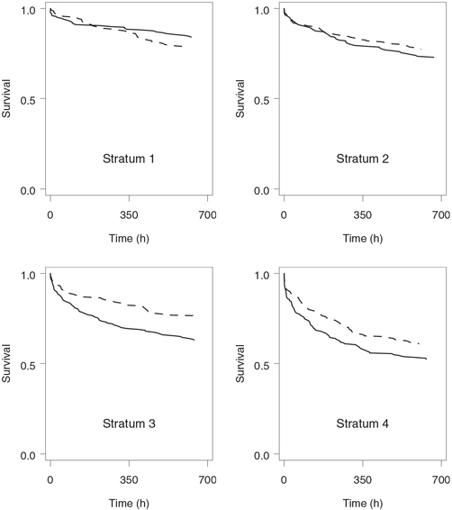
As an illustration, consider a clinical trial with a time-to-event endpoint comparing an experimental therapy to a placebo. Let t(1) < … < t(r) denote r ordered event times in the pooled sample. The magnitude of the distance between two survival functions is measured in the log-rank test using the statistic
dL=r∑k=1(d1k−e1k),
where d1k is the number of events observed in the experimental group at time t(k), and e1k is the expected number of events at time t(k) under the null hypothesis of no treatment effect on survival. We can see from the definition of dL that the deviations d1k — e1k, k = 1,…, r, are equally weighted in the log-rank test.
The Wilcoxon test is based on the idea that early events are more informative than those that occur later when few patients remain alive and survival curves are estimated with low precision. The Wilcoxon distance between two survival functions is given by
dW=r∑k=1nk(d1k−e1k),
where nk is the number of patients in the risk set before time t(k) (this includes patients who have not experienced the event of interest or have been censored before t(k)).
Similarly, the Tarone-Ware and Harrington-Fleming procedures are based on the distance statistics
dTW=r∑k=1n1/2k(d1k−e1k), dHF=r∑k=1Sρk(d1k−e1k),
respectively. Here Sk denotes the Kaplan-Meier estimate of the combined survival function of the two treatment groups at time t(k), and ρ is a parameter that determines how much weight is assigned to individual event times (0 ≤ ρ ≤ 1). The Tarone-Ware procedure represents the middle point between equally-weighted event times and a Wilcoxon weighting scheme giving considerably more weight to events that occurred early in the trial. To see this, note that the deviation d1k — e1k at time t(k) receives the weight of n0k=1 in the log-rank test and the weight of n1k=nk in the Wilcoxon test. The Harrington-Fleming procedure provides the statistician with a flexible balance between the log-rank-type and Wilcoxon-type weights. Letting ρ = 0 in the Harrington-Fleming procedure yields the log-rank test whereas letting ρ = 1 results in a test that assigns greater weights to early events.
An important consideration in selecting a statistical test is its efficiency against a particular alternative. The log-rank test is most powerful when the hazard functions in two treatment groups are proportional to each other, but it can be less efficient than the Wilcoxon test when the proportionality assumption is violated (Peto and Peto, 1972; Lee, Desu and Gehan, 1975; Prentice, 1978). It is generally difficult to characterize the alternative hypotheses that maximize the power of the Wilcoxon test because its efficiency depends on both survival and censoring distributions. It is known that the Wilcoxon test needs to be used with caution when early event times are heavily censored (Prentice and Marek, 1979). The Tarone-Ware procedure serves as a robust alternative to the log-rank and Wilcoxon procedures and maintains power better than these two procedures across a broad range of alternative hypotheses. Tarone and Ware (1977) demonstrated that their test is more powerful than the Wilcoxon test when the hazard functions are proportional and is more powerful than the log-rank test when the assumption of proportional hazards is not met. The same is true for the family of Harrington-Fleming tests.
Comparison of Survival Distributions Using the STRATA Statement in PROC LIFETEST
Randomization-based tests for homogeneity of survival distributions across treatment groups can be carried out using PROC LIFETEST by including the treatment group variable in either the STRATA or TEST statement. For example, Program 1.22 examines stratum-specific survival functions in the severe sepsis trial. In order to request a comparison of the two treatment groups (experimental drug versus placebo) within each stratum, the TREAT variable is included in the STRATA statement.
Program 1.22 Comparison of survival distributions in four strata using the STRATA statement
proc lifetest data=sepsurv notable;
ods select HomTests;
by stratum;
time survtime*censor(0);
strata treat;
run;
Output from Program 1.22
stratum=1
The LIFETEST Procedure
| Test of Equality over Strata | |||
| Test | Chi-Square | DF | Pr > Chi-Square |
| Log-Rank | 1.4797 | 1 | 0.2238 |
| Wilcoxon | 1.2748 | 1 | 0.2589 |
| -2Log(LR) | 1.6271 | 1 | 0.2021 |
stratum=2
The LIFETEST Procedure
| Test of Equality over Strata | |||
| Test | Chi-Square | DF | Pr > Chi-Square |
| Log-Rank | 0.9934 | 1 | 0.3189 |
| Wilcoxon | 0.8690 | 1 | 0.3512 |
| -2Log(LR) | 1.1345 | 1 | 0.2868 |
stratum=3
The LIFETEST Procedure
| Test of Equality over Strata | |||
| Test | Chi-Square | DF | Pr > Chi-Square |
| Log-Rank | 8.8176 | 1 | 0.0030 |
| Wilcoxon | 8.7611 | 1 | 0.0031 |
| -2Log(LR) | 10.3130 | 1 | 0.0013 |
stratum=4
The LIFETEST Procedure
| Test of Equality over Strata | |||
| Test | Chi-Square | DF | Pr > Chi-Square |
| Log-Rank | 3.5259 | 1 | 0.0604 |
| Wilcoxon | 3.9377 | 1 | 0.0472 |
| -2Log(LR) | 4.4858 | 1 | 0.0342 |
Including the TREAT variable in the STRATA statement results in a comparison of stratum-specific survival distributions based on the log-rank, Wilcoxon and likelihood ratio tests. Output 1.22 lists the log-rank, Wilcoxon and likelihood ratio statistics accompanied by asymptotic p-values. Note that extraneous information has been deleted from the output using the ODS statement (ods select HomTests). We can see from Output 1.22 that the treatment difference is far from being significant in Stratum 1 and Stratum 2, highly significant in Stratum 3 and marginally significant in Stratum 4. The three tests yield similar results within each stratum with the likelihood ratio statistic consistently being larger than the other two. Since the likelihood-ratio test is a parametric procedure that relies heavily on the assumption of an underlying exponential distribution, it needs to be used with caution unless one is certain that the exponential assumption is met.
Comparison of Survival Distributions Using the TEST Statement in PROC LIFETEST
An alternative approach to testing the significance of treatment effect on survival is based on the use of the TEST statement in PROC LIFETEST. If the treatment group variable is included in the TEST statement, PROC LIFETEST carries out only two tests (log-rank and Wilcoxon tests) to compare survival functions across treatment groups. The generated log-rank and Wilcoxon statistics are somewhat different from those shown in Output 1.22.
To illustrate, Program 1.23 computes the stratum-specific log-rank and Wilcoxon statistics and associated p-values when the TREAT variable is included in the TEST statement.
Program 1.23 Comparison of survival distributions in four strata using the TEST statement
proc lifetest data=sepsurv notable;
ods select LogUniChisq WilUniChiSq;
by stratum;
time survtime*censor(0);
test treat;
run;
Output from Program 1.23
stratum=1
Univariate Chi-Squares for the Wilcoxon Test
| Variable | Test Statistic | Standard Deviation | Chi-Square | Pr > Chi-Square |
| treat | -4.4090 | 3.9030 | 1.2761 | 0.2586 |
Univariate Chi-Squares for the Log-Rank Test
| Variable | Test Statistic | Standard Deviation | Chi-Square | Pr > Chi-Square |
| treat | -5.2282 | 4.3003 | 1.4781 | 0.2241 |
stratum=2
Univariate Chi-Squares for the Wilcoxon Test
| Variable | Test Statistic | Standard Deviation | Chi-Square | Pr > Chi-Square |
| treat | 4.0723 | 4.3683 | 0.8691 | 0.3512 |
Univariate Chi-Squares for the Log-Rank Test
| Variable | Test Statistic | Standard Deviation | Chi-Square | Pr > Chi-Square |
| treat | 4.9539 | 4.9743 | 0.9918 | 0.3193 |
stratum=3
Univariate Chi-Squares for the Wilcoxon Test
| Variable | Test Statistic | Standard Deviation | Chi-Square | Pr > Chi-Square |
| treat | 13.8579 | 4.6821 | 8.7602 | 0.0031 |
Univariate Chi-Squares for the Log-Rank Test
| Variable | Test Statistic | Standard Deviation | Chi-Square | Pr > Chi-Square |
| treat | 16.2909 | 5.4914 | 8.8007 | 0.0030 |
stratum=4
Univariate Chi-Squares for the Wilcoxon Test
| Variable | Test Statistic | Standard Deviation | Chi-Square | Pr > Chi-Square |
| treat | 10.3367 | 5.2107 | 3.9352 | 0.0473 |
Univariate Chi-Squares for the Log-Rank Test
| Variable | Test Statistic | Standard Deviation | Chi-Square | Pr > Chi-Square |
| treat | 12.3095 | 6.5680 | 3.5125 | 0.0609 |
Output 1.23 displays the Wilcoxon and log-rank statistics and p-values produced by Program 1.23. Note that the ODS statement (ods select LogUniChisq WilUniChiSq) is used to suppress a redundant set of Wilcoxon and log-rank statistics (under the headings “Forward Stepwise Sequence of Chi-Squares for the Log-Rank Test” and “Forward Stepwise Sequence of Chi-Squares for the Wilcoxon Test”) that would otherwise be included in the regular output. These stepwise procedures are identical to the univariate procedures shown above because only one variable was included in the TEST statement in Program 1.23.
It is easy to check that the stratum-specific log-rank and Wilcoxon statistics in Output 1.23 are a bit different from those shown in Output 1.22. The difference is fairly small but tends to increase with the value of a test statistic. To understand the observed discrepancy between the two sets of test statistics, one needs to remember that the TEST statement was added to PROC LIFETEST to enable the user to study effects of continuous covariates on survival distributions. The underlying testing procedures extend the log-rank and Wilcoxon tests for homogeneity of survival functions across treatment groups; see Kalbfleisch and Prentice (1980, Chapter 6). The more general versions of the log-rank and Wilcoxon tests do not always simplify to the ordinary tests when a categorical variable is included in the TEST statement. For example, if there were no identical survival times in the SEPSURV data set, the log-rank statistics in Output 1.23 would match those displayed in Output 1.22. Since this is not the case, the general version of the log-rank test implemented in PROC LIFETEST attempts to adjust for tied observations, which results in a slightly different value of the log-rank statistic. Analysis of time-to-event data with tied event times is discussed in more detail later in this section.
There is another way to look at the difference between inferences performed by PROC LIFETEST when the treatment group variable is included in the STRATA statement as opposed to the TEST statement. Roughly speaking, the tests listed in Output 1.22 (using the STRATA statement) represent a randomization-based testing method whereas the tests in Output 1.23 (using the TEST statement) are fairly closely related to a model-based approach. For example, it will be shown in Section 1.4.2 that the log-rank test in Output 1.23 is equivalent to a test based on the Cox proportional hazards model.
Comparison of Survival Distributions Using Tarone-Ware and Harrington-Fleming Tests
Thus far, we have focused on the log-rank, Wilcoxon and likelihood ratio testing procedures implemented in PROC LIFETEST. It is interesting to compare these procedures to the tests described by Tarone and Ware (1977) and Harrington and Fleming (1982). The latter tests can be implemented using the %LinRank macro written by Cantor (1997, Chapter 3) or, in SAS 9.1, they can be carried out directly in PROC LIFETEST. For example, the following code can be used in SAS 9.1 to compare survival distributions in the SEPSURV data set using the Tarone-Ware and Harrington-Fleming (ρ = 0.5) tests.
* Tarone-Ware and Harrington-Fleming tests in SAS 9.1;
proc lifetest data=sepsurv notable;
ods select HomTests;
by stratum;
time survtime*censor(0);
strata treat/test=(tarone fleming(0.5));
run;
The stratum-specific Tarone-Ware and Harrington-Fleming statistics and p-values produced by the %LinRank macro are summarized in Table 1.6. To facilitate the comparison with the log-rank and Wilcoxon tests computed in Program 1.22, the relevant test statistics and p-values from Output 1.22 are displayed at the bottom of the table.
Table 1.6 Comparison of the Tarone-Ware, Harrington-Fleming, log-rank and Wilcoxon tests
| Test | Stratum 1 | Stratum 2 | Stratum 3 | Stratum 4 |
| Tarone-Ware test | ||||
| Statistic | 1.3790 | 0.9331 | 8.8171 | 3.7593 |
| p-value | 0.2403 | 0.3341 | 0.0030 | 0.0525 |
| Harrington-Fleming test (ρ = 0.1) | ||||
| Statistic | 1.4599 | 0.9817 | 8.8220 | 3.5766 |
| p-value | 0.2269 | 0.3218 | 0.0030 | 0.0586 |
| Harrington-Fleming test (ρ = 1) | ||||
| Statistic | 1.2748 | 0.8690 | 8.7611 | 3.9377 |
| p-value | 0.2589 | 0.3512 | 0.0031 | 0.0472 |
| Log-rank test | ||||
| Statistic | 1.4797 | 0.9934 | 8.8176 | 3.5259 |
| p-value | 0.2238 | 0.3189 | 0.0030 | 0.0604 |
| Wilcoxon test | ||||
| Statistic | 1.2748 | 0.8690 | 8.7611 | 3.9377 |
| p-value | 0.2589 | 0.3512 | 0.0031 | 0.0472 |
Table 1.6 demonstrates that the p-values generated by the Tarone-Ware and Harrington-Fleming tests are comparable to the log-rank and Wilcoxon p-values computed in Program 1.22. By the definition of the Tarone-Ware procedure, the weights assigned to individual event times are greater than the log-rank weights and less than the Wilcoxon weights. As a consequence, the Tarone-Ware statistics lie between the corresponding log-rank and Wilcoxon statistics, and the Tarone-Ware procedure is always superior to the least powerful of these two procedures. When ρ = 0.1, the Harrington-Fleming weights are virtually independent of event times and thus the stratum-specific Harrington-Fleming statistics are generally close in magnitude to the log-rank statistics. On the other hand, the Harrington-Fleming weights approximate the Wilcoxon weights when ρ = 1, which causes the two sets of test statistics to be very close to each other.
Stratified Analysis of Time-to-Event Data
In the first part of this section we have concentrated on stratum-specific inferences; however, one is typically more interested in an overall analysis of the treatment effect controlling for important covariates. An adjusted effect of the experimental drug on a time-to-event outcome variable can be assessed by combining the information about the treatment differences across strata. PROC LIFETEST supports stratified versions of the Wilcoxon and log-rank tests. In order to carry out the stratified tests, one needs to include the treatment group variable in the TEST statement and add the stratification variable (e.g., baseline risk of death) to the STRATA statement.
Mathematically, stratified inferences performed by PROC LIFETEST are equivalent to pooling the Wilcoxon and log-rank distance statistics with equal weights across m strata. Specifically, let dLj denote the value of the log-rank distance between survival functions in the jth stratum and let s2Lj be the sample variance of dLj. The stratified log-rank statistic equals
uL=(m∑j=1dLj)2/m∑j=1s2Lj.
Under the null hypothesis that there is no difference in underlying survival distributions, the stratified statistic asymptotically follows a chi-square distribution with 1 degree of freedom. The stratified Wilcoxon statistic is defined in a similar manner.
Program 1.24 conducts the two stratified tests to evaluate the significance of treatment effect on survival in the severe sepsis trial adjusted for the baseline risk of mortality.
Program 1.24 Stratified comparison of survival distributions in four strata using the Wilcoxon and log-rank tests
proc lifetest data=sepsurv notable;
ods select LogUniChisq WilUniChiSq;
time survtime*censor(0);
strata stratum;
test treat;
run;
Output from Program 1.24
Univariate Chi-Squares for the Wilcoxon Test
| Variable | Test Statistic | Standard Deviation | Chi-Square | Pr > Chi-Square |
| treat | 23.8579 | 9.1317 | 6.8259 | 0.0090 |
Univariate Chi-Squares for the Log-Rank Test
| Variable | Test Statistic | Standard Deviation | Chi-Square | Pr > Chi-Square |
| treat | 28.3261 | 10.7949 | 6.8855 | 0.0087 |
Output 1.24 shows the stratified Wilcoxon and log-rank statistics and p-values produced by Program 1.24. As in Program 1.23, the ODS statement is used (ods select LogUniChisq WilUniChiSq) to display the relevant sections of the PROC LIFETEST output. The stratified Wilcoxon and log-rank p-values are 0.0090 and 0.0087, respectively. The two p-values are almost identical and indicate that the adjusted effect of the experimental drug on survival is very strong. It is worth noting that the stratified Wilcoxon and log-rank statistics are much larger than the corresponding statistics computed in Strata 1, 2 and 4 (see Output 1.23). As expected, stratification increases the power of the testing procedures.
We can also compare the computed stratified Wilcoxon and log-rank p-values to those produced by the stratified Tarone-Ware and Harrington-Fleming tests. From the %LinRank macro, the stratified Tarone-Ware statistic is 6.8975 (p = 0.0086) and the stratified Harrington-Fleming statistic equals 6.9071 (p = 0.0086) if ρ = 0.1, and 6.8260 (p = 0.0090) if ρ = 1. The obtained results are in good agreement with the stratified analysis based on the Wilcoxon and log-rank tests.