
5.8.6 SAS Procedures for Multiple Imputation
As mentioned before, PROC MI is used to generate the imputations. It creates M imputed data sets, physically stored in a single data set with indicator _IMPUTATION_ to separate the various imputed copies from each other. We will describe some options available in the PROC MI statement. The option SIMPLE displays simple descriptive statistics and pairwise correlations based on available cases in the input data set. The number of imputations is specified by NIMPUTE and is by default equal to 5. The option ROUND controls the number of decimal places in the imputed values (by default there is no rounding). If more than one number is specified, one should use a VAR statement, and the specified numbers must correspond to variables in the VAR statement. The SEED option specifies a positive integer, which is used by PROC MI to start the pseudo-random number generator. The default is a value generated from the time of day on the computer’s clock. The imputation task is carried out separately for each level of the BY variables. In PROC MI, we can choose between one of the three imputation mechanisms we discussed in Section 5.8.5. For monotone missingness only, we use the MONOTONE statement. The parametric regression method (METHOD=REG) as well as the nonparametric propensity score method (METHOD=PROPENSITY) is available. For general patterns of missingness, we use the MCMC statement (the MCMC method is the default one). In all cases, several options are available to control the procedures; MCMC especially has a great deal of flexibility. For instance, NGROUPS specifies the number of groups based on propensity scores when the propensity scores method is used. For the MCMC method, we can give the initial mean and covariance estimates to begin the MCMC process by INITIAL. The PMM option in the MCMC statement uses the predictive mean matching method to impute an observed value that is closest to the predicted value in the MCMC method. The REGPMM option in the MONOTONE statement uses the predictive mean matching method to impute an observed value that is closest to the predicted value for data sets with monotone missingness. One can specify more than one method in the MONOTONE statement, and for each imputed variable the covariates can be specified separately. With INITIAL=EM (default), PROC MI uses the means and standard deviations from available cases as the initial estimates for the EM algorithm. The resulting estimates are used to begin the MCMC process. You can also specify INITIAL= input SAS data set to use a SAS data set with the initial estimates of the mean and covariance matrix for each imputation. Further, NITER specifies the number of iterations between imputations in a single chain (default is equal to 30).
The experimental CLASS statement is available since SAS 9.0 and is intended to specify categorical variables. Such classification variables are used as either covariates for imputed variables or as imputed variables for data sets with monotone missing patterns.
An important addition since SAS 9.0 are the experimental options LOGISTIC and DISCRIM in the MONOTONE statement, used to impute missing categorical variables by logistic and discriminant methods, respectively.
After the imputations have been generated, the imputed data sets are analyzed using a standard procedure. It is important to ensure that the BY statement is used to force an analysis for each of the imputed sets of data separately. Appropriate output (estimates and the precision thereof) is stored in output data sets.
Finally, PROC MIANALYZE combines the M inferences into a single one by making use of the theory laid out in Section 5.8.2. The options PARMS=. and COVB=., or their counterparts stemming from other standard procedures, name an input SAS data set that contains parameter estimates, and respectively covariance matrices of the parameter estimates, from the imputed data sets. The VAR statement lists the variables to be analyzed; they must be numeric. This statement is required.
This procedure is straightforward in a number of standard cases, such as PROC REG, PROC CORR, PROC GENMOD, PROC GLM, and PROC MIXED (for fixed effects in the cross-sectional case), but it is less straightforward in the PROC MIXED case when data are longitudinal or when interest is also in the variance components.
The experimental (since SAS 9.0) CLASS statement specifies categorical variables. PROC MIANALYZE reads and combines parameter estimates and covariance matrices for parameters with CLASS variables. The TEST statement allows testing of hypotheses about linear combinations of the parameters. The statement is based on Rubin (1987) and uses a t distribution that is the univariate version of the work by Li, Raghunathan and Rubin (1991), described in Section 5.8.3.
EXAMPLE: Growth Data
To begin, we show the standard, direct-likelihood-based MAR analysis using the PROC MIXED program for the GROWTH data set Model 7, which turned out to be the most parsimonious model (see Section 5.7).
Program 5.12 Direct-likelihood-based MAR analysis for Model 7
proc mixed data=growthax asycov covtest;
title "Standard proc mixed analysis";
class idnr age sex;
model measure=age*sex /noint solution covb;
repeated age /subject=idnr type=cs;
run;
To perform this analysis using multiple imputation, the data need to be organized horizontally (one record per subject) rather than vertically. This can be done with the next program. A part of the horizontal data set obtained with this program is also given.
Program 5.13 Data manipulation for the imputation task
data hulp1;
set growthax;
meas8=measure;
if age=8 then output;
run;
data hulp2;
set growthax;
meas10=measure;
if age=10 then output;
run;
data hulp3;
set growthax;
meas12=measure;
if age=12 then output;
run;
data hulp4;
set growthax;
meas14=measure;
if age=14 then output;
run;
data growthmi;
merge hulp1 hulp3 hulp4 hulp2;
run;
proc sort data=growthmi;
by sex;
proc print data=growthmi;
title "Horizontal data set";
run;
Horizontal data set
| Obs | IDNR | INDIV | AGE | SEX | MEASURE | MEAS8 | MEAS12 | MEAS14 | MEAS10 |
| 1 | 12 | 1 | 10 | 1 | 25.0 | 26.0 | 29.0 | 31.0 | 25.0 |
| 2 | 13 | 2 | 10 | 1 | . | 21.5 | 23.0 | 26.5 | . |
| 3 | 14 | 3 | 10 | 1 | 22.5 | 23.0 | 24.0 | 27.5 | 22.5 |
| 4 | 15 | 4 | 10 | 1 | 27.5 | 25.5 | 26.5 | 27.0 | 27.5 |
| 5 | 16 | 5 | 10 | 1 | . | 20.0 | 22.5 | 26.0 | . |
| ... | |||||||||
The data are now ready for the so-called imputation task. This is done by PROC MI in the next program. Note that the measurement times are ordered as (8,12,14,10), since age 10 is incomplete. In this way, a monotone ordering is achieved. In line with the earlier analysis, we will use the monotone regression method.
Program 5.14 Imputation task
proc mi data=growthmi seed=459864 simple nimpute=10
round=0.1 out=outmi;
by sex;
monotone method=reg;
var meas8 meas12 meas14 meas10;
run;
We show some output of the MI procedure for SEX=1. First, some pattern-specific information is given. Since we included the option SIMPLE, univariate statistics and pairwise correlations are calculated (not shown). Finally, multiple imputation variance information shows the total variance and the magnitudes of between and within variance.
Output from Program 5.14 (partial)
| ----------------SEX=1 ---------------- | ||||||
| Missing Data Patterns | ||||||
| Group | MEAS8 | MEAS12 | MEAS14 | MEAS10 | Freq | Percent |
| 1 | X | X | X | X | 11 | 68.75 |
| 2 | X | X | X | . | 5 | 31.25 |
| --------------Group Means-------------- | ||||
| Group | MEAS8 | MEAS12 | MEAS14 | MEAS10 |
| 1 | 24.000000 | 26.590909 | 27.681818 | 24.136364 |
| 2 | 20.400000 | 23.800000 | 27.000000 | . |
Multiple Imputation Variance Information
| --------------Variance-------------- | ||||
| Variable | Between | Within | Total | DF |
| MEAS10 | 0.191981 | 0.865816 | 1.076995 | 10.25 |
| Relative | Fraction | |
| Increase | Missing | |
| Variable | in Variance | Information |
| MEAS10 | 0.243907 | 0.202863 |
Multiple Imputation Parameter Estimates
| Variable | Mean | Std Error | 95% Confidence | Limits | DF | |
| MEAS10 | 22.685000 | 1.037784 | 20.38028 | 24.98972 | 10.25 | |
| Variable | Minimum | Maximum | Mu0 | t for H0: Mean=Mu0 |
Pr > |t| | |
| MEAS10 | 21.743750 | 23.387500 | 0 | 21.86 | <.0001 | |
A selection of the imputed data set is shown below (first four observations, imputations 1 and 2). To prepare for a standard linear mixed model analysis (using PROC MIXED), a number of further data manipulation steps are conducted, including the construction of a vertical data set with one record per measurement and not one record per subject (i.e., back to the original format). Part of the imputed data set in vertical format is also given.
Portion of imputed data set in horizontal format
| Obs | _Imp_ | IDNR | INDIV | AGE | SEX | MEASURE | MEAS8 | MEAS12 | MEAS14 | MEAS10 |
| 1 | 1 | 1 | 1 | 10 | 2 | 20.0 | 21.0 | 21.5 | 23.0 | 20.0 |
| 2 | 1 | 2 | 2 | 10 | 2 | 21.5 | 21.0 | 24.0 | 25.5 | 21.5 |
| 3 | 1 | 3 | 3 | 10 | 2 | . | 20.5 | 24.5 | 26.0 | 22.6 |
| 4 | 1 | 4 | 4 | 10 | 2 | 24.5 | 23.5 | 25.0 | 26.5 | 24.5 |
| 28 | 2 | 1 | 1 | 10 | 2 | 20.0 | 21.0 | 21.5 | 23.0 | 20.0 |
| 29 | 2 | 2 | 2 | 10 | 2 | 21.5 | 21.0 | 24.0 | 25.5 | 21.5 |
| 30 | 2 | 3 | 3 | 10 | 2 | . | 20.5 | 24.5 | 26.0 | 20.4 |
| 31 | 2 | 4 | 4 | 10 | 2 | 24.5 | 23.5 | 25.0 | 26.5 | 24.5 |
Program 5.15 Data manipulation to use PROC MIXED
proc sort data=outmi;
by_imputation_ idnr;
run;
proc print data=outmi;
title ’Horizontal imputed data set’;
run;
data outmi2;
set outmi;
array y (4) meas8 meas10 meas12 meas14;
do j=1 to 4;
measmi=y(j);
age=6+2*j;
output;
end;
run;
proc print data=outmi2;
title "Vertical imputed data set";
run;
Portion of imputed data set in vertical format
| Obs | _Imp_ | IDNR | INDIV | AGE | SEX | MEASURE | MEAS8 | MEAS12 | MEAS14 | MEAS10 | j | measmi |
| 1 | 1 | 1 | 1 | 8 | 2 | 20.0 | 21.0 | 21.5 | 23.0 | 20.0 | 1 | 21.0 |
| 2 | 1 | 1 | 1 | 10 | 2 | 20.0 | 21.0 | 21.5 | 23.0 | 20.0 | 2 | 20.0 |
| 3 | 1 | 1 | 1 | 12 | 2 | 20.0 | 21.0 | 21.5 | 23.0 | 20.0 | 3 | 21.5 |
| 4 | 1 | 1 | 1 | 14 | 2 | 20.0 | 21.0 | 21.5 | 23.0 | 20.0 | 4 | 23.0 |
| 5 | 1 | 2 | 2 | 8 | 2 | 21.5 | 21.0 | 24.0 | 25.5 | 21.5 | 1 | 21.0 |
| 6 | 1 | 2 | 2 | 10 | 2 | 21.5 | 21.0 | 24.0 | 25.5 | 21.5 | 2 | 21.5 |
| 7 | 1 | 2 | 2 | 12 | 2 | 21.5 | 21.0 | 24.0 | 25.5 | 21.5 | 3 | 24.0 |
| 8 | 1 | 2 | 2 | 14 | 2 | 21.5 | 21.0 | 24.0 | 25.5 | 21.5 | 4 | 25.5 |
| 9 | 1 | 3 | 3 | 8 | 2 | . | 20.5 | 24.5 | 26.0 | 22.6 | 1 | 20.5 |
| 10 | 1 | 3 | 3 | 10 | 2 | . | 20.5 | 24.5 | 26.0 | 22.6 | 2 | 22.6 |
| 11 | 1 | 3 | 3 | 12 | 2 | . | 20.5 | 24.5 | 26.0 | 22.6 | 3 | 24.5 |
| 12 | 1 | 3 | 3 | 14 | 2 | . | 20.5 | 24.5 | 26.0 | 22.6 | 4 | 26.0 |
After the imputation step and additional data manipulation, the imputed data sets can be analyzed using the MIXED procedure. Using the ODS statement, four sets of input for the inference task (i.e., the combination of all inferences into a single one) are preserved:
• parameter estimates of the fixed effects: MIXBETAP
• parameter estimates of the variance components: MIXALFAP
• covariance matrix of the fixed effects: MIXBETAV
• covariance matrix of the variance components: MIXALFAV.
Program 5.16 Analysis of imputed data sets using PROC MIXED
proc mixed data=outmi2 asycov;
title "Multiple Imputation Call of PROC MIXED"
class idnr age sex;
model measmi=age*sex /noint solution covb;
repeated age /subject=idnr type=cs;
by_Imputation_;
ods output solutionF=mixbetap covb=mixbetav
covparms=mixalfap asycov=mixalfav;
run;
proc print data=mixbetap;
title "Fixed effects: parameter estimates";
run;
proc print data=mixbetav;
title "Fixed effects: variance-covariance matrix";
run;
proc print data=mixalfav;
title "Variance components: covariance parameters";
run;
proc print data=mixalfap;
title "Variance components: parameter estimates";
run;
We show a selection of the output from the PROC MIXED call on imputation 1. We also show part of the fixed effects estimates data set and part of the data set of the variance-covariance matrices of the fixed effects (both imputations 1 and 2), as well as the estimates of the covariance parameters and their covariance matrices. However, in order to call PROC MIANALYZE, one parameter vector and one covariance matrix (per imputation) need to be passed on, with the proper name. This requires, once again, some data manipulation.
Output from Program 5.16 (partial)
| ----------Imputation Number=1---------- |
| Covariance Parameter Estimates | ||
| Cov Parm | Subject | Estimate |
| CS | IDNR | 3.7019 |
| Residual | 2.1812 | |
Asymptotic Covariance Matrix of Estimates
| Row | Cov Parm | CovP1 | CovP2 |
| 1 | CS | 1.4510 | -0.03172 |
| 2 | Residual | -0.03172 | 0.1269 |
Solution for Fixed Effects
| Effect | AGE | SEX | Estimate | Standard Error |
DF | t Value | Pr > |t| |
| AGE*SEX | 8 | 1 | 22.8750 | 0.6064 | 73 | 37.72 | <.0001 |
| AGE*SEX | 8 | 2 | 21.0909 | 0.7313 | 73 | 28.84 | <.0001 |
| AGE*SEX | 10 | 1 | 23.3875 | 0.6064 | 73 | 38.57 | <.0001 |
| AGE*SEX | 10 | 2 | 22.1273 | 0.7313 | 73 | 30.26 | <.0001 |
| AGE*SEX | 12 | 1 | 25.7188 | 0.6064 | 73 | 42.41 | <.0001 |
| AGE*SEX | 12 | 2 | 22.6818 | 0.7313 | 73 | 31.01 | <.0001 |
| AGE*SEX | 14 | 1 | 27.4688 | 0.6064 | 73 | 45.30 | <.0001 |
| AGE*SEX | 14 | 2 | 24.0000 | 0.7313 | 73 | 32.82 | <.0001 |
Covariance Matrix for Fixed Effects
| Row | Effect | AGE | SEX | Col1 | Col2 | Col3 | Col4 | Col5 |
| 1 | AGE*SEX | 8 | 1 | 0.3677 | 0.2314 | 0.2314 | ||
| 2 | AGE*SEX | 8 | 2 | 0.5348 | 0.3365 | |||
| 3 | AGE*SEX | 10 | 1 | 0.2314 | 0.3677 | 0.2314 | ||
| 4 | AGE*SEX | 10 | 2 | 0.3365 | 0.5348 | |||
| 5 | AGE*SEX | 12 | 1 | 0.2314 | 0.2314 | 0.3677 | ||
| 6 | AGE*SEX | 12 | 2 | 0.3365 | 0.3365 | |||
| 7 | AGE*SEX | 14 | 1 | 0.2314 | 0.2314 | 0.2314 | ||
| 8 | AGE*SEX | 14 | 2 | 0.3365 | 0.3365 |
| Row | Col6 | Col7 | Col8 |
| 1 | 0.2314 | ||
| 2 | 0.3365 | 0.3365 | |
| 3 | 0.2314 | ||
| 4 | 0.3365 | 0.3365 | |
| 5 | 0.2314 | ||
| 6 | 0.5348 | 0.3365 | |
| 7 | 0.3677 | ||
| 8 | 0.3365 | 0.5348 | |
Type 3 Tests of Fixed Effects
| Effect | Num DF | Den DF | F Value | Pr > F |
| AGE*SEX | 8 | 73 | 469.91 | <.0001 |
Part of the fixed effects estimates data set
| Obs | _Imputation_ | Effect | AGE | SEX | Estimate | StdErr | DF | tValue | Probt |
| 1 | 1 | AGE*SEX | 8 | 1 | 22.8750 | 0.6064 | 73 | 37.72 | <.0001 |
| 2 | 1 | AGE*SEX | 8 | 2 | 21.0909 | 0.7313 | 73 | 28.84 | <.0001 |
| 3 | 1 | AGE*SEX | 10 | 1 | 23.3875 | 0.6064 | 73 | 38.57 | <.0001 |
| 4 | 1 | AGE*SEX | 10 | 2 | 22.1273 | 0.7313 | 73 | 30.26 | <.0001 |
| 5 | 1 | AGE*SEX | 12 | 1 | 25.7188 | 0.6064 | 73 | 42.41 | <.0001 |
| 6 | 1 | AGE*SEX | 12 | 2 | 22.6818 | 0.7313 | 73 | 31.01 | <.0001 |
| 7 | 1 | AGE*SEX | 14 | 1 | 27.4688 | 0.6064 | 73 | 45.30 | <.0001 |
| 8 | 1 | AGE*SEX | 14 | 2 | 24.0000 | 0.7313 | 73 | 32.82 | <.0001 |
| 9 | 2 | AGE*SEX | 8 | 1 | 22.8750 | 0.6509 | 73 | 35.15 | <.0001 |
| 10 | 2 | AGE*SEX | 8 | 2 | 21.0909 | 0.7850 | 73 | 26.87 | <.0001 |
| 11 | 2 | AGE*SEX | 10 | 1 | 22.7438 | 0.6509 | 73 | 34.94 | <.0001 |
| 12 | 2 | AGE*SEX | 10 | 2 | 21.8364 | 0.7850 | 73 | 27.82 | <.0001 |
| 13 | 2 | AGE*SEX | 12 | 1 | 25.7188 | 0.6509 | 73 | 39.52 | <.0001 |
| 14 | 2 | AGE*SEX | 12 | 2 | 22.6818 | 0.7850 | 73 | 28.90 | <.0001 |
| 15 | 2 | AGE*SEX | 14 | 1 | 27.4688 | 0.6509 | 73 | 42.20 | <.0001 |
| 16 | 2 | AGE*SEX | 14 | 2 | 24.0000 | 0.7850 | 73 | 30.57 | <.0001 |
| ... | |||||||||
Part of the data set of the variance-covariance matrices of the fixed effects
| Obs | _Imputation_ | Row | Effect | AGE | SEX | Col1 | Col2 | Col3 |
| 1 | 1 | 1 | AGE*SEX | 8 | 1 | 0.3677 | 0 | 0.2314 |
| 2 | 1 | 2 | AGE*SEX | 8 | 2 | 0 | 0.5348 | 0 |
| 3 | 1 | 3 | AGE*SEX | 10 | 1 | 0.2314 | 0 | 0.3677 |
| 4 | 1 | 4 | AGE*SEX | 10 | 2 | 0 | 0.3365 | 0 |
| 5 | 1 | 5 | AGE*SEX | 12 | 1 | 0.2314 | 0 | 0.2314 |
| 6 | 1 | 6 | AGE*SEX | 12 | 2 | 0 | 0.3365 | 0 |
| 7 | 1 | 7 | AGE*SEX | 14 | 1 | 0.2314 | 0 | 0.2314 |
| 8 | 1 | 8 | AGE*SEX | 14 | 2 | 0 | 0.3365 | 0 |
| 9 | 2 | 1 | AGE*SEX | 8 | 1 | 0.4236 | 0 | 0.2504 |
| 10 | 2 | 2 | AGE*SEX | 8 | 2 | 0 | 0.6162 | 0 |
| 11 | 2 | 3 | AGE*SEX | 10 | 1 | 0.2504 | 0 | 0.4236 |
| 12 | 2 | 4 | AGE*SEX | 10 | 2 | 0 | 0.3642 | 0 |
| 13 | 2 | 5 | AGE*SEX | 12 | 1 | 0.2504 | 0 | 0.2504 |
| 14 | 2 | 6 | AGE*SEX | 12 | 2 | 0 | 0.3642 | 0 |
| 15 | 2 | 7 | AGE*SEX | 14 | 1 | 0.2504 | 0 | 0.2504 |
| 16 | 2 | 8 | AGE*SEX | 14 | 2 | 0 | 0.3642 | 0 |
| ... | ||||||||
| Obs | Col4 | Col5 | Col6 | Col7 | Col8 |
| 1 | 0 | 0.2314 | 0 | 0.2314 | 0 |
| 2 | 0.3365 | 0 | 0.3365 | 0 | 0.3365 |
| 3 | 0 | 0.2314 | 0 | 0.2314 | 0 |
| 4 | 0.5348 | 0 | 0.3365 | 0 | 0.3365 |
| 5 | 0 | 0.3677 | 0 | 0.2314 | 0 |
| 6 | 0.3365 | 0 | 0.5348 | 0 | 0.3365 |
| 7 | 0 | 0.2314 | 0 | 0.3677 | 0 |
| 8 | 0.3365 | 0 | 0.3365 | 0 | 0.5348 |
| 9 | 0 | 0.2504 | 0 | 0.2504 | 0 |
| 10 | 0.3642 | 0 | 0.3642 | 0 | 0.3642 |
| 11 | 0 | 0.2504 | 0 | 0.2504 | 0 |
| 12 | 0.6162 | 0 | 0.3642 | 0 | 0.3642 |
| 13 | 0 | 0.4236 | 0 | 0.2504 | 0 |
| 14 | 0.3642 | 0 | 0.6162 | 0 | 0.3642 |
| 15 | 0 | 0.2504 | 0 | 0.4236 | 0 |
| 16 | 0.3642 | 0 | 0.3642 | 0 | 0.6162 |
| ... | |||||
Estimates of the covariance parameters in the original data set form
| Obs | _Imputation_ | CovParm | Subject | Estimate |
| 1 | 1 | CS | IDNR | 3.7019 |
| 2 | 1 | Residual | 2.1812 | |
| 3 | 2 | CS | IDNR | 4.0057 |
| 4 | 2 | Residual | 2.7721 | |
| 5 | 3 | CS | IDNR | 4.5533 |
| 6 | 3 | Residual | 4.3697 | |
| 7 | 4 | CS | IDNR | 4.0029 |
| 8 | 4 | Residual | 2.7910 | |
| 9 | 5 | CS | IDNR | 4.1198 |
| 10 | 5 | Residual | 2.7918 | |
| 11 | 6 | CS | IDNR | 4.0549 |
| 12 | 6 | Residual | 3.0254 | |
| 13 | 7 | CS | IDNR | 3.9019 |
| 14 | 7 | Residual | 3.2477 | |
| 15 | 8 | CS | IDNR | 4.3877 |
| 16 | 8 | Residual | 2.9076 | |
| 17 | 9 | CS | IDNR | 4.0192 |
| 18 | 9 | Residual | 3.6492 | |
| 19 | 10 | CS | IDNR | 3.8346 |
| 20 | 10 | Residual | 2.1826 |
Covariance matrices of the covariance parameters in the original data set form
| Obs | _Imputation_ | Row | CovParm | CovP1 | CovP2 |
| 1 | 1 | 1 | CS | 1.4510 | -0.03172 |
| 2 | 1 | 2 | Residual | -0.03172 | 0.1269 |
| 3 | 2 | 1 | CS | 1.7790 | -0.05123 |
| 4 | 2 | 2 | Residual | -0.05123 | 0.2049 |
| 5 | 3 | 1 | CS | 2.5817 | -0.1273 |
| 6 | 3 | 2 | Residual | -0.1273 | 0.5092 |
| 7 | 4 | 1 | CS | 1.7807 | -0.05193 |
| 8 | 4 | 2 | Residual | -0.05193 | 0.2077 |
| 9 | 5 | 1 | CS | 1.8698 | -0.05196 |
| 10 | 5 | 2 | Residual | -0.05196 | 0.2078 |
| 11 | 6 | 1 | CS | 1.8671 | -0.06102 |
| 12 | 6 | 2 | Residual | -0.06102 | 0.2441 |
| 13 | 7 | 1 | CS | 1.7952 | -0.07032 |
| 14 | 7 | 2 | Residual | -0.07032 | 0.2813 |
| 15 | 8 | 1 | CS | 2.1068 | -0.05636 |
| 16 | 8 | 2 | Residual | -0.05636 | 0.2254 |
| 17 | 9 | 1 | CS | 1.9678 | -0.08878 |
| 18 | 9 | 2 | Residual | -0.08878 | 0.3551 |
| 19 | 10 | 1 | CS | 1.5429 | -0.03176 |
| 20 | 10 | 2 | Residual | -0.03176 | 0.1270 |
Program 5.17 Data manipulation for the inference task
data mixbetap0;
set mixbetap;
if age= 8 and sex=1 then effect=’as081’;
if age=10 and sex=1 then effect=’as101’;
if age=12 and sex=1 then effect=’as121’;
if age=14 and sex=1 then effect=’as141’;
if age= 8 and sex=2 then effect=’as082’;
if age=10 and sex=2 then effect=’as102’;
if age=12 and sex=2 then effect=’as122’;
if age=14 and sex=2 then effect=’as142’;
run;
data mixbetap0;
set mixbetap0 (drop=age sex);
run;
proc print data=mixbetap0;
title "Fixed effects: parameter estimates (after manipulation)";
run;
data mixbetav0;
set mixbetav;
if age= 8 and sex=1 then effect=’as081’;
if age=10 and sex=1 then effect=’as101’;
if age=12 and sex=1 then effect=’as121’;
if age=14 and sex=1 then effect=’as141’;
if age= 8 and sex=2 then effect=’as082’;
if age=10 and sex=2 then effect=’as102’;
if age=12 and sex=2 then effect=’as122’;
if age=14 and sex=2 then effect=’as142’;
run;
data mixbetav0;
title "Fixed effects: variance-covariance matrix (after manipulation)";
set mixbetav0 (drop=row age sex);
run;
proc print data=mixbetav0;
run;
data mixalfap0;
set mixalfap;
effect=covparm;
run;
data mixalfav0;
set mixalfav;
effect=covparm;
Col1=CovP1;
Col2=CovP2;
run;
proc print data=mixalfap0;
title "Variance components: parameter estimates
(after manipulation)";
run;
proc print data=mixalfav0;
title "Variance components: covariance parameters
(after manipulation)";
run;
The following outputs show parts of the data sets after this data manipulation.
Part of the fixed effects estimates data set after data manipulation
| Obs | _Imputation_ | Effect | Estimate | StdErr | DF | tValue | Probt |
| 1 | 1 | as081 | 22.8750 | 0.6064 | 73 | 37.72 | <.0001 |
| 2 | 1 | as082 | 21.0909 | 0.7313 | 73 | 28.84 | <.0001 |
| 3 | 1 | as101 | 23.3875 | 0.6064 | 73 | 38.57 | <.0001 |
| 4 | 1 | as102 | 22.1273 | 0.7313 | 73 | 30.26 | <.0001 |
| 5 | 1 | as121 | 25.7188 | 0.6064 | 73 | 42.41 | <.0001 |
| 6 | 1 | as122 | 22.6818 | 0.7313 | 73 | 31.01 | <.0001 |
| 7 | 1 | as141 | 27.4688 | 0.6064 | 73 | 45.30 | <.0001 |
| 8 | 1 | as142 | 24.0000 | 0.7313 | 73 | 32.82 | <.0001 |
| 9 | 2 | as081 | 22.8750 | 0.6509 | 73 | 35.15 | <.0001 |
| 10 | 2 | as082 | 21.0909 | 0.7850 | 73 | 26.87 | <.0001 |
| 11 | 2 | as101 | 22.7438 | 0.6509 | 73 | 34.94 | <.0001 |
| 12 | 2 | as102 | 21.8364 | 0.7850 | 73 | 27.82 | <.0001 |
| 13 | 2 | as121 | 25.7188 | 0.6509 | 73 | 39.52 | <.0001 |
| 14 | 2 | as122 | 22.6818 | 0.7850 | 73 | 28.90 | <.0001 |
| 15 | 2 | as141 | 27.4688 | 0.6509 | 73 | 42.20 | <.0001 |
| 16 | 2 | as142 | 24.0000 | 0.7850 | 73 | 30.57 | <.0001 |
| ... | |||||||
Part of the data set of the variance-covariance matrices of the fixed effects after data manipulation
| Obs | _Imputation_ | Effect | Col1 | Col2 | Col3 |
| 1 | 1 | as081 | 0.3677 | 0 | 0.2314 |
| 2 | 1 | as082 | 0 | 0.5348 | 0 |
| 3 | 1 | as101 | 0.2314 | 0 | 0.3677 |
| 4 | 1 | as102 | 0 | 0.3365 | 0 |
| 5 | 1 | as121 | 0.2314 | 0 | 0.2314 |
| 6 | 1 | as122 | 0 | 0.3365 | 0 |
| 7 | 1 | as141 | 0.2314 | 0 | 0.2314 |
| 8 | 1 | as142 | 0 | 0.3365 | 0 |
| 9 | 2 | as081 | 0.4236 | 0 | 0.2504 |
| 10 | 2 | as082 | 0 | 0.6162 | 0 |
| 11 | 2 | as101 | 0.2504 | 0 | 0.4236 |
| 12 | 2 | as102 | 0 | 0.3642 | 0 |
| 13 | 2 | as121 | 0.2504 | 0 | 0.2504 |
| 14 | 2 | as122 | 0 | 0.3642 | 0 |
| 15 | 2 | as141 | 0.2504 | 0 | 0.2504 |
| 16 | 2 | as142 | 0 | 0.3642 | 0 |
| ... | |||||
| Obs | Col4 | Col5 | Col6 | Col7 | Col8 |
| 1 | 0 | 0.2314 | 0 | 0.2314 | 0 |
| 2 | 0.3365 | 0 | 0.3365 | 0 | 0.3365 |
| 3 | 0 | 0.2314 | 0 | 0.2314 | 0 |
| 4 | 0.5348 | 0 | 0.3365 | 0 | 0.3365 |
| 5 | 0 | 0.3677 | 0 | 0.2314 | 0 |
| 6 | 0.3365 | 0 | 0.5348 | 0 | 0.3365 |
| 7 | 0 | 0.2314 | 0 | 0.3677 | 0 |
| 8 | 0.3365 | 0 | 0.3365 | 0 | 0.5348 |
| 9 | 0 | 0.2504 | 0 | 0.2504 | 0 |
| 10 | 0.3642 | 0 | 0.3642 | 0 | 0.3642 |
| 11 | 0 | 0.2504 | 0 | 0.2504 | 0 |
| 12 | 0.6162 | 0 | 0.3642 | 0 | 0.3642 |
| 13 | 0 | 0.4236 | 0 | 0.2504 | 0 |
| 14 | 0.3642 | 0 | 0.6162 | 0 | 0.3642 |
| 15 | 0 | 0.2504 | 0 | 0.4236 | 0 |
| 16 | 0.3642 | 0 | 0.3642 | 0 | 0.6162 |
| ... | |||||
Estimates of the covariance parameters after manipulation, i.e., addition of an ’effect’ column (identical to the ’CovParm’ column)
| Obs | _Imputation_ | CovParm | Subject | Estimate | effect |
| 1 | 1 | CS | IDNR | 3.7019 | CS |
| 2 | 1 | Residual | 2.1812 | Residual | |
| 3 | 2 | CS | IDNR | 4.0057 | CS |
| 4 | 2 | Residual | 2.7721 | Residual | |
| 5 | 3 | CS | IDNR | 4.5533 | CS |
| 6 | 3 | Residual | 4.3697 | Residual | |
| 7 | 4 | CS | IDNR | 4.0029 | CS |
| 8 | 4 | Residual | 2.7910 | Residual | |
| 9 | 5 | CS | IDNR | 4.1198 | CS |
| 10 | 5 | Residual | 2.7918 | Residual | |
| 11 | 6 | CS | IDNR | 4.0549 | CS |
| 12 | 6 | Residual | 3.0254 | Residual | |
| 13 | 7 | CS | IDNR | 3.9019 | CS |
| 14 | 7 | Residual | 3.2477 | Residual | |
| 15 | 8 | CS | IDNR | 4.3877 | CS |
| 16 | 8 | Residual | 2.9076 | Residual | |
| 17 | 9 | CS | IDNR | 4.0192 | CS |
| 18 | 9 | Residual | 3.6492 | Residual | |
| 19 | 10 | CS | IDNR | 3.8346 | CS |
| 20 | 10 | Residual | 2.1826 | Residual |
Covariance matrices of the covariance parameters after manipulation, i.e., addition of an ’effect’ column (identical to the ’CovParm’ column)
| Obs | _Imputation_ | Row | CovParm | CovP1 | CovP2 | effect | Col1 | Col2 |
| 1 | 1 | 1 | CS | 1.4510 | -0.03172 | CS | 1.45103 | -0.03172 |
| 2 | 1 | 2 | Residual | -0.03172 | 0.1269 | Residual | -0.03172 | 0.12688 |
| 3 | 2 | 1 | CS | 1.7790 | -0.05123 | CS | 1.77903 | -0.05123 |
| 4 | 2 | 2 | Residual | -0.05123 | 0.2049 | Residual | -0.05123 | 0.20492 |
| 5 | 3 | 1 | CS | 2.5817 | -0.1273 | CS | 2.58173 | -0.12729 |
| 6 | 3 | 2 | Residual | -0.1273 | 0.5092 | Residual | -0.12729 | 0.50918 |
| 7 | 4 | 1 | CS | 1.7807 | -0.05193 | CS | 1.78066 | -0.05193 |
| 8 | 4 | 2 | Residual | -0.05193 | 0.2077 | Residual | -0.05193 | 0.20772 |
| 9 | 5 | 1 | CS | 1.8698 | -0.05196 | CS | 1.86981 | -0.05196 |
| 10 | 5 | 2 | Residual | -0.05196 | 0.2078 | Residual | -0.05196 | 0.20784 |
| 11 | 6 | 1 | CS | 1.8671 | -0.06102 | CS | 1.86710 | -0.06102 |
| 12 | 6 | 2 | Residual | -0.06102 | 0.2441 | Residual | -0.06102 | 0.24409 |
| 13 | 7 | 1 | CS | 1.7952 | -0.07032 | CS | 1.79518 | -0.07032 |
| 14 | 7 | 2 | Residual | -0.07032 | 0.2813 | Residual | -0.07032 | 0.28127 |
| 15 | 8 | 1 | CS | 2.1068 | -0.05636 | CS | 2.10683 | -0.05636 |
| 16 | 8 | 2 | Residual | -0.05636 | 0.2254 | Residual | -0.05636 | 0.22544 |
| 17 | 9 | 1 | CS | 1.9678 | -0.08878 | CS | 1.96778 | -0.08878 |
| 18 | 9 | 2 | Residual | -0.08878 | 0.3551 | Residual | -0.08878 | 0.35510 |
| 19 | 10 | 1 | CS | 1.5429 | -0.03176 | CS | 1.54287 | -0.03176 |
| 20 | 10 | 2 | Residual | -0.03176 | 0.1270 | Residual | -0.03176 | 0.12703 |
Now, PROC MIANALYZE will be called, first for the fixed effects inferences, and then for the variance component inferences. The parameter estimates (MIXBETAP0) and the covariance matrix (MIXBETAV0) are the input for the fixed effects. Output is given following the program. For the fixed effects, there is only between-imputation variability for the age 10 measurement. However, for the variance components, we see that covariance parameters are influenced by missingness.
Program 5.18 Inference task using PROC MIANALYZE
proc mianalyze parms=mixbetap0 covb=mixbetav0;
title "Multiple Imputation Analysis for Fixed Effects";
var as081 as082 as101 as102 as121 as122 as141 as142;
run;
proc mianalyze parms=mixalfap0 covb=mixalfav0;
title "Multiple Imputation Analysis for Variance Components";
var CS Residual;
run;
Output from Program 5.18 (fixed effects)
| Model Information | |
| PARMS Data Set | WORK.MIXBETAP0 |
| COVB Data Set | WORK.MIXBETAV0 |
| Number of Imputations | 10 |
Multiple Imputation Variance Information
| --------------Variance-------------- | ||||
| Parameter | Between | Within | Total | DF |
| as081 | 0 | 0.440626 | 0.440626 | . |
| as082 | 0 | 0.640910 | 0.640910 | . |
| as101 | 0.191981 | 0.440626 | 0.651804 | 85.738 |
| as102 | 0.031781 | 0.640910 | 0.675868 | 3364 |
| as121 | 0 | 0.440626 | 0.440626 | . |
| as122 | 0 | 0.640910 | 0.640910 | . |
| as141 | 0 | 0.440626 | 0.440626 | . |
| as142 | 0 | 0.640910 | 0.640910 | . |
| Multiple Imputation Variance Information | ||
| Parameter | Relative Increase in Variance |
Information Fraction Missing Information |
| as081 | 0 | . |
| as082 | 0 | . |
| as101 | 0.479271 | 0.339227 |
| as102 | 0.054545 | 0.052287 |
| as121 | 0 | . |
| as122 | 0 | . |
| as141 | 0 | . |
| as142 | 0 | . |
Multiple Imputation Parameter Estimates
| Parameter | Estimate | Std Error | 95% Confidence | Limits | DF |
| as081 | 22.875000 | 0.663796 | . | . | . |
| as082 | 21.090909 | 0.800568 | . | . | . |
| as101 | 22.685000 | 0.807344 | 21.07998 | 24.29002 | 85.738 |
| as102 | 22.073636 | 0.822112 | 20.46175 | 23.68553 | 3364 |
| as121 | 25.718750 | 0.663796 | . | . | . |
| as122 | 22.681818 | 0.800568 | . | . | . |
| as141 | 27.468750 | 0.663796 | . | . | . |
| as142 | 24.000000 | 0.800568 | . | . | . |
Multiple Imputation Parameter Estimates
| Parameter | Minimum | Maximum |
| as081 | 22.875000 | 22.875000 |
| as082 | 21.090909 | 21.090909 |
| as101 | 21.743750 | 23.387500 |
| as102 | 21.836364 | 22.381818 |
| as121 | 25.718750 | 25.718750 |
| as122 | 22.681818 | 22.681818 |
| as141 | 27.468750 | 27.468750 |
| as142 | 24.000000 | 24.000000 |
Multiple Imputation Parameter Estimates
| Parameter | Theta0 | t for H0: Parameter=Theta0 |
Pr > |t| |
| as081 | 0 | . | . |
| as082 | 0 | . | . |
| as101 | 0 | 28.10 | <.0001 |
| as102 | 0 | 26.85 | <.0001 |
| as121 | 0 | . | . |
| as122 | 0 | . | . |
| as141 | 0 | . | . |
| as142 | 0 | . | . |
Output from Program 5.18 (variance components)
Model Information
| PARMS Data Set | WORK.MIXALFAP0 |
| COVB Data Set | WORK.MIXALFAV0 |
| Number of Imputations | 10 |
Multiple Imputation Variance Information
| --------------Variance-------------- | ||||
| Parameter | Between | Within | Total | DF |
| CS | 0.062912 | 1.874201 | 1.943404 | 7097.8 |
| Residual | 0.427201 | 0.248947 | 0.718868 | 21.062 |
Multiple Imputation Variance Information
| Parameter | Relative Increase in Variance |
Fraction Missing Information |
| CS | 0.036924 | 0.035881 |
| Residual | 1.887630 | 0.682480 |
Multiple Imputation Parameter Estimates
| Parameter | Estimate | Std Error | 95% Confidence | Limits | DF |
| CS | 4.058178 | 1.394060 | 1.325404 | 6.790951 | 7097.8 |
| Residual | 2.991830 | 0.847861 | 1.228921 | 4.754740 | 21.062 |
Multiple Imputation Parameter Estimates
| Parameter | Minimum | Maximum |
| CS | 3.701888 | 4.553271 |
| Residual | 2.181247 | 4.369683 |
Multiple Imputation Parameter Estimates
| Parameter | Theta0 | t for H0: Parameter=Theta0 |
Pr > |t| |
| CS | 0 | 2.91 | 0.0036 |
| Residual | 0 | 3.53 | 0.0020 |
It is clear that multiple imputation has an impact on the precision of the age 10 measurement, the only time at which incompleteness occurs. The manipulations are rather extensive, given that multiple imputation was used not only for fixed effects parameters, but also for variance components, in a genuinely longitudinal application. The main reason for the large amount of manipulation is to ensure input datasets have format and column headings in line with what is expected by PROC MIANALYZE. The take-home message is that, when one is prepared to undertake a bit of data manipulation, PROC MI and PROC MIANALYZE provide a valuable couple of procedures that enable multiple imputation in a wide variety of settings.
5.8.7 Creating Monotone Missingness
When missingness is nonmonotone, one might think of several mechanisms operating simultaneously: e.g., a simple (MCAR or MAR) mechanism for the intermediate missing values and a more complex (MNAR) mechanism for the missing data past the moment of dropout. However, analyzing such data is complicated because many model strategies, especially those under the assumption of MNAR, have been developed for dropout only. Therefore, a solution might be to generate multiple imputations that render the data sets monotone missing by including the following statement in PROC MI:
mcmc impute = monotone;
and then applying a method of choice to the multiple sets of data that are thus completed. Note that this is different from the monotone method in PROC MI, intended to fully complete already monotone sets of data.
5.9 The EM Algorithm
This section deals with the expectation-maximization algorithm, popularly known as the EM algorithm. It is an alternative to direct likelihood in settings where the observed-data likelihood is complicated and/or difficult to access. Note that direct likelihood is within reach for many settings, including Gaussian longitudinal data, as outlined in Section 5.7.
The EM algorithm is a general-purpose iterative algorithm to find maximum likelihood estimates in parametric models for incomplete data. Within each iteration of the EM algorithm, there are two steps, called the expectation step, or E-step, and the maximization step, or M-step. The name EM algorithm was given by Dempster, Laird and Rubin (1977), who provided a general formulation of the EM algorithm, its basic properties, and many examples and applications of it. The books by Little and Rubin (1987), Schafer (1997), and McLachlan and Krishnan (1997) provide detailed descriptions and applications of the EM algorithm.
The basic idea of the EM algorithm is to associate with the given incomplete data problem a complete data problem for which maximum likelihood estimation is computationally more tractable. Starting from suitable initial parameter values, the E- and M-steps are repeated until convergence. Given a set of parameter estimates—such as the mean vector and covariance matrix for a multivariate normal setting—the E-step calculates the conditional expectation of the complete data log-likelihood given the observed data and the parameter estimates. This step is often reduced to simple sufficient statistics. Given the complete data log-likelihood, the M-step then finds the parameter estimates to maximize the complete data log-likelihood from the E-step.
An initial criticism was that the EM algorithm did not produce estimates of the covariance matrix of the maximum likelihood estimators. However, developments have provided methods for such estimation that can be integrated into the EM computational procedures. Another issue is the slow convergence in certain cases. This has resulted in the development of modified versions of the algorithm as well as many simulated-based methods and other extensions of it (McLachlan and Krishnan, 1997).
The condition for the EM algorithm to be valid, in its basic form, is ignorability and hence MAR.
5.9.1 The Algorithm
The Initial Step
Let θ(0) be an initial parameter vector, which can be found, for example, from a complete case analysis, an available case analysis, or a simple method of imputation.
The E-Step
Given current values θ(t) for the parameters, the E-step computes the objective function, which in the case of the missing data problem is equal to the expected value of the observed-data log-likelihood, given the observed data and the current parameters
Q(θ|θ(t))=∫ℓ(θ,Y)f(Ym|Y0,θ(t))dYm=E[ℓ(θ|Y)|Y0,θ(t)],
i.e., substituting the expected value of Ym, given Yo and θ(t). In some cases, this substitution can take place directly at the level of the data, but often it is sufficient to substitute only the function of Ym appearing in the complete-data log-likelihood. For exponential families, the E-step reduces to the computation of complete-data sufficient statistics.
The M-Step
The M-step determines θ(t+1), the parameter vector maximizing the log-likelihood of the imputed data (or the imputed log-likelihood). Formally, θ(t+1)satisfies
Q(θ(t+1)|θ(t))≥Q(θ|θ(t)), for all θ
One can show that the likelihood increases at every step. Since the log-likelihood is bounded from above, convergence is forced to apply.
The fact that the EM algorithm is guaranteed of convergence to a possibly local maximum is a great advantage. However, a disadvantage is that this convergence is slow (linear or superlinear), and that precision estimates are not automatically provided.
5.9.2 Missing Information
We will now turn attention to the principle of missing information. We use obvious notation for the observed and expected information matrices for the complete and observed data. Let
I(θ,Y0)=∂2In ℓ(θ)∂θ∂θ′
be the matrix of the negative of the second-order partial derivatives of the incomplete-data log-likelihood function with respect to the elements of θ, i.e., the observed information matrix for the observed data model. The expected information matrix for observed data model is termed I(θ,Y0). In analogy with the complete data Y=(Y0,Ym), we let Ic(θ,Y) and Ic(θ,Y) be the observed and expected information matrices for the complete data model, respectively. Now, both likelihoods are connected via
ℓ(θ)=ℓc(θ)−In fc(y0,ym|θ)fc(y0|θ)=ℓc(θ)−In f(ym|y0,θ).
This equality carries over onto the information matrices:
I(θ,Y0)=Ic(θ,Y)+∂2In f(ym|y0,θ)∂θ∂θ′.
Taking expectation over Y|Y0=y0 leads to
I(θ,y0)=Ic(θ,y0)−Im(θ,y0),
where Im(θ, y0) is the expected information matrix for θ based on Ym when conditioned on Yo. This information can be viewed as the “missing information,” resulting from observing Yo only and not also Ym. This leads to the missing information principle
Ic(θ,y)=I(θ,y)+Im(θ,y),
which has the following interpretation: the (conditional expected) complete information equals the observed information plus the missing information.
5.9.3 Rate of Convergence
The notion that the rate at which the EM algorithm converges depends upon the amount of missing information in the incomplete data compared to the hypothetical complete data will be made explicit by deriving results regarding the rate of convergence in terms of information matrices.
Under regularity conditions, the EM algorithm will converge linearly. By using a Taylor series expansion we can write
θ(t+1)−θ*≃J(θ*)[θ(t)−θ*].
Thus, in a neighborhood of θ*, the EM algorithm is essentially a linear iteration with rate matrix J(θ*), since J(θ*) is typically nonzero. For this reason, J(θ*) is often referred to as the matrix rate of convergence, or simply the rate of convergence. For vector θ*, a measure of the actual observed convergence rate is the global rate of convergence, which can be assessed by
r=limt→∞‖θ(t+1)−θ*‖‖θ(t)−θ*‖,
where ||.|| is any norm on d-dimensional Euclidean space ℝd, and d is the number of missing values. In practice, during the process of convergence, r is typically assessed as
r=limt→∞‖θ(t+1)−θ(t)‖‖θ(t)−θ(t−1)‖.
Under regularity conditions, it can be shown that r is the largest eigenvalue of the d × d rate matrix J(θ*).
Now, J(θ*) can be expressed in terms of the observed and missing information:
J(θ*)=Id−Ic(θ*,Y0)−1I(θ*,Y0)=Ic(θ*,Y0)−1Im(θ*,Y0).
This means the rate of convergence of the EM algorithm is given by the largest eigenvalue of the information ratio matrix Ic(θ,Y0)−1Im(θ,Y0), which measures the proportion of information about θ that is missing as a result of not also observing Ym in addition to Yo. The greater the proportion of missing information, the slower the rate of convergence. The fraction of information loss may vary across different components of θ, suggesting that certain components of θ may approach θ* rapidly using the EM algorithm, while other components may require a large number of iterations. Further, exceptions to the convergence of the EM algorithm to a local maximum of the likelihood function occur if J(θ *) has eigenvalues exceeding unity.
5.9.4 EM Acceleration
Using the concept of rate matrix
θ(t+1)−θ*≃J(θ*)[θ(t)−θ*],
we can solve this for θ*, to yield
˜θ*=(Id−J)−1(θ(t+1)−Jθ(t)).
The J matrix can be determined empirically, using a sequence of subsequent iterations. It also follows from the observed and complete or, equivalently, missing information:
J=Id−Ic(θ*,Y)−1I(θ*,Y).
Here, ˜θ* can then be seen as an accelerated iteration.
5.9.5 Calculation of Precision Estimates
The observed information matrix is not directly accessible. It has been shown by Louis (1982) that
Im(θ,Y0)=E[Sc(θ,Y)Sc(θ,Y)′|y0]−S(θ,Y0)S(θ,Y0)′.
This leads to an expression for the observed information matrix in terms of quantities that are available (McLachlan and Krishnan, 1997):
I(θ,Y)=Im(θ,Y)−E[Sc(θ,Z)Sc(θ,Z)′|y]+S(θ,Y)S(θ,Y)′.
From this equation, the observed information matrix can be computed as
I(ˆθ,Y)=Im(ˆθ,Y)−E[Sc(ˆθ,Z)Sc(ˆθ,Z)′|y],
where θ̂ is the maximum likelihood estimator.
5.9.6 EM Algorithm Using SAS
A version of the EM algorithm for both multivariate normal and categorical data can be conducted using the MI procedure in SAS. Indeed, with the MCMC imputation method (for general nonmonotone settings), the MCMC chain is started using EM-based starting values. It is possible to suppress the actual MCMC-based multiple imputation, thus restricting action of PROC MI to the EM algorithm.
The NIMPUTE option in the MI procedure should be set equal to zero. This means the multiple imputation will be skipped, and only tables of model information, missing data patterns, descriptive statistics (in case the SIMPLE option is given) and the MLE from the EM algorithm (EM statement) are displayed.
We have to specify the EM statement so that the EM algorithm is used to compute the maximum likelihood estimate (MLE) of the data with missing values, assuming a multivariate normal distribution for the data. The following five options are available with the EM statement. The option CONVERGE=. sets the convergence criterion. The value must be between 0 and 1. The iterations are considered to have converged when the maximum change in the parameter estimates between iteration steps is less than the value specified. The change is a relative change if the parameter is greater than 0.01 in absolute value; otherwise it is an absolute change. By default, CONVERGE=1E-4. The iteration history in the EM algorithm is printed if the option ITPRINT is given. The maximum number of iterations used in the EM algorithm is specified with the MAXITER=. option. The default is MAXITER=200. The option OUTEM=. creates an output SAS data set containing the MLE of the parameter vector (μ,), computed with the EM algorithm. Finally, OUTITER=. creates an output SAS data set containing parameters for each iteration. The data set includes a variable named ITERATION to identify the iteration number.
PROC MI uses the means and standard deviations from the available cases as the initial estimates for the EM algorithm. The correlations are set equal to zero.
EXAMPLE: Growth Data
Using the horizontal version of the GROWTH data set created in Section 5.8, we can use the following program:
Program 5.19 The EM algorithm using PROC MI
proc mi data=growthmi seed=495838 simple nimpute=0;
em itprint outem=growthem1;
var meas8 meas12 meas14 meas10;
by sex;
run;
Part of the output generated by this program (for SEX=1) is given below. The procedure displays the initial parameter estimates for EM, the iteration history (because option ITPRINT is given), and the EM parameter estimates, i.e., the maximum likelihood estimates for μ and Σ from the incomplete GROWTH data set.
Output from Program 5.19 (SEX=1 group)
| ------------------SEX=1 ------------------ | |||||
| Initial Parameter Estimates for EM | |||||
| _TYPE_ | _NAME_ | MEAS8 | MEAS12 | MEAS14 | MEAS10 |
| MEAN | 22.875000 | 25.718750 | 27.468750 | 24.136364 | |
| COV | MEAS8 | 6.016667 | 0 | 0 | 0 |
| COV | MEAS12 | 0 | 7.032292 | 0 | 0 |
| COV | MEAS14 | 0 | 0 | 4.348958 | 0 |
| COV | MEAS10 | 0 | 0 | 0 | 5.954545 |
EM (MLE) Iteration History
| _Iteration_ | -2 Log L | MEAS10 |
| 0 | 158.065422 | 24.136364 |
| 1 | 139.345763 | 24.136364 |
| 2 | 138.197324 | 23.951784 |
| 3 | 137.589135 | 23.821184 |
| 4 | 137.184304 | 23.721865 |
| 5 | 136.891453 | 23.641983 |
| . | ||
| . | ||
| . | ||
| 42 | 136.070697 | 23.195650 |
| 43 | 136.070694 | 23.195453 |
| 44 | 136.070693 | 23.195285 |
| 45 | 136.070692 | 23.195141 |
| 46 | 136.070691 | 23.195018 |
| 47 | 136.070690 | 23.194913 |
EM (MLE) Parameter Estimates
| _TYPE_ | _NAME_ | MEAS8 | MEAS12 | MEAS14 | MEAS10 |
| MEAN | 22.875000 | 25.718750 | 27.468750 | 23.194913 | |
| COV | MEAS8 | 5.640625 | 3.402344 | 1.511719 | 5.106543 |
| COV | MEAS12 | 3.402344 | 6.592773 | 3.038086 | 2.555289 |
| COV | MEAS14 | 1.511719 | 3.038086 | 4.077148 | 1.937547 |
| COV | MEAS10 | 5.106543 | 2.555289 | 1.937547 | 7.288687 |
EM (Posterior Mode) Estimates
| _TYPE_ | _NAME_ | MEAS8 | MEAS12 | MEAS14 | MEAS10 |
| MEAN | 22.875000 | 25.718750 | 27.468750 | 23.194535 | |
| COV | MEAS8 | 4.297619 | 2.592262 | 1.151786 | 3.891806 |
| COV | MEAS12 | 2.592262 | 5.023065 | 2.314732 | 1.947220 |
| COV | MEAS14 | 1.151786 | 2.314732 | 3.106399 | 1.476056 |
| COV | MEAS10 | 3.891806 | 1.947220 | 1.476056 | 5.379946 |
One can also output the EM parameter estimates into an output data set with the OUTEM=. option. A printout of the GROWTHEM1 data set produces a handy summary for both sexes:
Summary for both sex groups
| Obs | SEX | _TYPE_ | _NAME_ | MEAS8 | MEAS12 | MEAS14 | MEAS10 |
| 1 | 1 | MEAN | 22.8750 | 25.7188 | 27.4688 | 23.1949 | |
| 2 | 1 | COV | MEAS8 | 5.6406 | 3.4023 | 1.5117 | 5.1065 |
| 3 | 1 | COV | MEAS12 | 3.4023 | 6.5928 | 3.0381 | 2.5553 |
| 4 | 1 | COV | MEAS14 | 1.5117 | 3.0381 | 4.0771 | 1.9375 |
| 5 | 1 | COV | MEAS10 | 5.1065 | 2.5553 | 1.9375 | 7.2887 |
| 6 | 2 | MEAN | 21.0909 | 22.6818 | 24.0000 | 22.0733 | |
| 7 | 2 | COV | MEAS8 | 4.1281 | 5.0744 | 4.3636 | 2.9920 |
| 8 | 2 | COV | MEAS12 | 5.0744 | 7.5579 | 6.6591 | 3.9260 |
| 9 | 2 | COV | MEAS14 | 4.3636 | 6.6591 | 6.6364 | 3.1666 |
| 10 | 2 | COV | MEAS10 | 2.9920 | 3.9260 | 3.1666 | 2.9133 |
Should we want to combine this program with genuine multiple imputation, then the program can be augmented as follows (using the MCMC default):
Program 5.20 Combining EM algorithm and multiple imputation
proc mi data=growthmi seed=495838 simple nimpute=5 out=growthmi2;
em itprint outem=growthem2;
var meas8 meas12 meas14 meas10;
by sex;
run;
5.10 Categorical Data
The non-Gaussian setting is different in the sense that there is no generally accepted counterpart to the linear mixed effects model. We therefore first sketch a general taxonomy for longitudinal models in this context, including marginal, random effects (or subject-specific), and conditional models. We then argue that marginal and random effects models both have their merit in the analysis of longitudinal clinical trial data and focus on two important representatives: the generalized estimating equations (GEE) approach within the marginal family and the generalized linear mixed effects model (GLMM) within the random effects family. We highlight important similarities and differences between these model families. While GLMM parameters can be fitted using maximum likelihood, the same is not true for the frequentist GEE method. Therefore, Robins, Rotnitzky and Zhao (1995) have devised so-called weighted generalized estimating equations (WGEE), valid under MAR but requiring the specification of a dropout model in terms of observed outcomes and/or covariates in order to specify the weights.
5.10.1 Discrete Repeated Measures
We distinguish between several generally nonequivalent extensions of univariate models. In a marginal model, marginal distributions are used to describe the outcome vector Y, given a set X of predictor variables. The correlation among the components of Y can then be captured either by adopting a fully parametric approach or by means of working assumptions, such as in the semiparametric approach of Liang and Zeger (1986). Alternatively, in a random effects model, the predictor variables X are supplemented with a vector θ of random effects, conditional upon which the components of Y are usually assumed to be independent. This does not preclude that more elaborate models are possible if residual dependence is detected (Longford, 1993). Finally, a conditional model describes the distribution of the components of Y, conditional on X but also conditional on a subset of the other components of Y. Well-known members of this class of models are log-linear models (Gilula and Haberman, 1994).
Marginal and random effects models are two important subfamilies of models for repeated measures. Several authors, such as Diggle et al. (2002) and Aerts et al. (2002) distinguish between three such families. Still focusing on continuous outcomes, a marginal model is characterized by the specification of a marginal mean function
E(Yij|xij)=x′ijβ,(5.18)
whereas in a random effects model we focus on the expectation, conditional upon the random effects vector:
E(Yij|bi,xij)=x′ijβ+z′ijbi.(5.19)
Finally, a third family of models conditions a particular outcome on the other responses or a subset thereof. In particular, a simple first-order stationary transition model focuses on expectations of the form
E(Yij|Yi,j−1,…,Yi1,xij)=x′ijβ+αYi,j−1.(5.20)
In the linear mixed model case, random effects models imply a simple marginal model. This is due to the elegant properties of the multivariate normal distribution. In particular, the expectation described in equation (5.18) follows from equation (5.19) by either (a) marginalizing over the random effects or by (b) conditioning upon the random effects vector bi = 0. Hence, the fixed effects parameters β have both a marginal as well as a hierarchical model interpretation. Finally, when a conditional model is expressed in terms of residuals rather than outcomes directly, it also leads to particular forms of the general linear mixed effects model.
Such a close connection between the model families does not exist when outcomes are of a nonnormal type, such as binary, categorical, or discrete. We will consider each of the model families in turn and then point to some particular issues arising within them or when comparisons are made between them.
5.10.2 Marginal Models
In marginal models, the parameters characterize the marginal probabilities of a subset of the outcomes without conditioning on the other outcomes. Advantages and disadvantages of conditional and marginal modeling have been discussed in Diggle et al. (2002) and Fahrmeir and Tutz (2002). The specific context of clustered binary data has received treatment in Aerts et al. (2002). Apart from full likelihood approaches, nonlikelihood approaches, such as generalized estimating equations (Liang and Zeger, 1986) or pseudo-likelihood (le Cessie and van Houwelingen, 1994; Geys, Molenberghs and Lipsitz, 1998) have been considered.
Bahadur (1961) proposed a marginal model, accounting for the association via marginal correlations. Ekholm (1991) proposed a so-called success probabilities approach. George and Bowman (1995) proposed a model for the particular case of exchangeable binary data. Ashford and Sowden (1970) considered the multivariate probit model for repeated ordinal data, thereby extending univariate probit regression. Molenberghs and Lesaffre (1994) and Lang and Agresti (1994) have proposed models which parameterize the association in terms of marginal odds ratios. Dale (1986) defined the bivariate global odds ratio model, based on a bivariate Plackett distribution (Plackett, 1965). Molenberghs and Lesaffre (1994, 1999) extended this model to multivariate ordinal outcomes. They generalize the bivariate Plackett distribution in order to establish the multivariate cell probabilities. Their 1994 method involves solving polynomials of high degree and computing the derivatives thereof, while in 1999 generalized linear models theory is exploited, together with the use of an adaption of the iterative proportional fitting algorithm. Lang and Agresti (1994) exploit the equivalence between direct modeling and imposing restrictions on the multinomial probabilities, using undetermined Lagrange multipliers. Alternatively, the cell probabilities can be fitted using a Newton iteration scheme, as suggested by Glonek and McCullagh (1995). We will consider generalized estimating equations (GEE) and weighted generalized estimating equations (WGEE) in turn.
Generalized Estimating Equations
The main issue with full likelihood approaches is the computational complexity they entail. When we are mainly interested in first-order marginal mean parameters and pairwise association parameters—i.e., second-order moments—a full likelihood procedure can be replaced by quasi-likelihood methods (McCullagh and Nelder, 1989). In quasi-likelihood, the mean response is expressed as a parametric function of covariates; the variance is assumed to be a function of the mean up to possibly unknown scale parameters. Wedderburn (1974) first noted that likelihood and quasi-likelihood theories coincide for exponential families and that the quasi-likelihood estimating equations provide consistent estimates of the regression parameters β in any generalized linear model, even for choices of link and variance functions that do not correspond to exponential families.
For clustered and repeated data, Liang and Zeger (1986) proposed so-called generalized estimating equations (GEE or GEE1) which require only the correct specification of the univariate marginal distributions provided one is willing to adopt working assumptions about the association structure. They estimate the parameters associated with the expected value of an individual’s vector of binary responses and phrase the working assumptions about the association between pairs of outcomes in terms of marginal correlations. The method combines estimating equations for the regression parameters β with moment-based estimating for the correlation parameters entering the working assumptions.
Prentice (1988) extended their results to allow joint estimation of probabilities and pairwise correlations. Lipsitz, Laird and Harrington (1991) modified the estimating equations of Prentice to allow modeling of the association through marginal odds ratios rather than marginal correlations. When adopting GEE1 one does not use information of the association structure to estimate the main effect parameters. As a result, it can be shown that GEE1 yields consistent main effect estimators, even when the association structure is misspecified. However, severe misspecification may seriously affect the efficiency of the GEE1 estimators. In addition, GEE1 should be avoided when some scientific interest is placed on the association parameters.
A second order extension of these estimating equations (GEE2) that includes the marginal pairwise association as well has been studied by Liang, Zeger and Qaqish (1992). They note that GEE2 is nearly fully efficient, though bias may occur in the estimation of the main effect parameters when the association structure is misspecified.
Usually, when confronted with the analysis of clustered or otherwise correlated data, conclusions based on mean parameters (e.g., dose effect) are of primary interest. When inferences for the parameters in the mean model E(yi) are based on classical maximum likelihood theory, full specification of the joint distribution for the vector yi of repeated measurements within each unit i is necessary. For discrete data, this implies specification of the first-order moments as well as all higher-order moments and, depending on whether marginal or random effects models are used, assumptions are either explicitly made or implicit in the random effects structure. For Gaussian data, full-model specification reduces to modeling the first- and second-order moments only. However, even then inappropriate covariance models can seriously invalidate inferences for the mean structure. Thus, a drawback of a fully parametric model is that incorrect specification of nuisance characteristics can lead to invalid conclusions about key features of the model.
After this short overview of the GEE approach, the GEE methodology, which is based on two principles, will now be explained a little further. First, the score equations to be solved when computing maximum likelihood estimates under a marginal normal model yi∼N(Xiβ,Vi) are given by
N∑i=1X′i(A1/2iRiA1/2i)−1(yi−Xiβ)=0,(5.21)
in which the marginal covariance matrix Vi has been decomposed in the form A1/2iRiA1/2i, with Ai the matrix with the marginal variances on the main diagonal and zeros elsewhere, and with Ri equal to the marginal correlation matrix. Second, the score equations to be solved when computing maximum likelihood estimates under the marginal generalized linear model (5.18), assuming independence of the responses within units (i.e., ignoring the repeated measures structure), are given by
N∑i=1∂μi∂β′(A1/2iIniA1/2i)−1(yi−μi)=0,(5.22)
where Ai is again the diagonal matrix with the marginal variances on the main diagonal.
Note that expression (5.21) has the same form as expression (5.22) but with the correlations between repeated measures taken into account. A straightforward extension of expression (5.22) that accounts for the correlation structure is
S(β)N∑i=1∂μi∂β′(A1/2iRiA1/2i)−1(yi−μi)=0,(5.23)
which is obtained from replacing the identity matrix Ini with a correlation matrix Ri=Ri(α), often referred to as the working correlation matrix. Usually, the marginal covariance matrix Vi=A1/2iRiA1/2i contains a vector α of unknown parameters which is replaced for practical purposes by a consistent estimate.
Assuming that the marginal mean μi has been correctly specified as h(μi)=Xiβ, it can be shown that, under mild regularity conditions, the estimator ˆβ obtained from solving expression (5.23) is asymptotically normally distributed with mean β and with covariance matrix
I−10I1I−10,(5.24)
where
I0=(N∑i=1∂μ′i∂βV−11∂μi∂β′),I1=(N∑i=1∂μ′i∂βV−11Var(yi)V−1i∂μi∂β′).
In practice, Var(yi) in the matrix (5.24) is replaced by (yi−μi)(yi−μi)′, which is unbiased on the sole condition that the mean was again correctly specified.
Note that valid inferences can now be obtained for the mean structure, only assuming that the model assumptions with respect to the first-order moments are correct. Note also that, although arising from a likelihood approach, the GEE equations in expression (5.23) cannot be interpreted as score equations corresponding to some full likelihood for the data vector yi.
Liang and Zeger (1986) proposed moment-based estimates for the working correlation. To this end, first define deviations
eij=yij−μij√v(μij)
and decompose the variance slightly more generally as above in the following way:
Vi=ϕA1/2iRiA1/2i,
where φ is an overdispersion parameter.
Some of the more popular choices for the working correlations are independence (Corr(Yij,Yik)=0, j≠k), exchangeability (Corr(Yij,Yik)=α, j≠k), AR(1) (Corr(Yij,Yi,j+t)=αt, t=0,1,…,ni−j), and unstructured (Corr(Yij,Yik)=αjk, j≠k). Typically, moment-based estimation methods are used to estimate these parameters, as part of an integrated iterative estimation procedure (Aerts et al., 2002). The overdispersion parameter is approached in a similar fashion. The standard iterative procedure to fit GEE, based on Liang and Zeger (1986), is then as follows: (1) compute initial estimates for β, using a univariate GLM (i.e., assuming independence); (2) compute the quantities needed in the estimating equation: bi; (3) compute Pearson residuals eij; (4) compute estimates for α ; (5) compute Ri (α); (6) compute an estimate for ϕ; (7) compute Vi(β,α)=ϕA1/2i(β)Ri(α)A1/2i(β). (8) update the estimate for β :
β(t+1)=β(t)−[N∑i=1∂μ′i∂βV−11∂μi∂β]−1[N∑i=1∂μ′i∂βV−11(yi−μi)].
Steps (2) through (8) are iterated until convergence.
Weighted Generalized Estimating Equations
The problem of dealing with missing values is common throughout statistical work and is almost always present in the analysis of longitudinal or repeated measurements. For categorical outcomes, as we have seen before, the GEE approach could be adapted. However, as Liang and Zeger (1986) pointed out, inferences with the GEE are valid only under the strong assumption that the data are missing completely at random (MCAR). To allow the data to be missing at random (MAR), Robins, Rotnitzky and Zhao (1995) proposed a class of weighted estimating equations. They can be viewed as an extension of generalized estimating equations.
The idea is to weight each subject’s measurements in the GEEs by the inverse probability that a subject drops out at that particular measurement occasion. This can be calculated as
vit≡P[Di=t]=t−1Πk=2(1−P[Rik=0|Ri2=…=Ri,k−1=1])ΧP[Rit=0|Ri2=…=Ri,t−1=1]I{t≤T}
if dropout occurs by time t or we reach the end of the measurement sequence, and
vit≡P[Di=t]=tΠk=2(1−P[Rik=0|Ri2=…=Ri,k−1=1])
otherwise. Recall that we partitioned Yi into the unobserved components Ymi and the observed components Y0i. Similarly, we can make the exact same partition of μi into μmi and μ0i. In the weighted GEE approach, which is proposed to reduce possible bias of ˆβ, the score equations to be solved when taking into account the correlation structure are:
S(β)=N∑i=11vi∂μi∂β′(A1/2iRiA1/2i)−1(yi−μi)=0
or
S(β)=N∑i=1n+1∑d=21(Di=d)vid∂μi∂β′(d)(A1/2iRiA1/2i)−1(d)(yi(d)−μi(d))=0,
where yi (d) and μi (d) are the first d – 1 elements of yi and μi respectively. We define ∂μi∂β′(d) and (A1/2iRiA1/2i)−1(d) analogously, in line with the definition of Robins, Rotnitzky and Zhao (1995).
5.10.3 Random Effects Models
Models with subject-specific parameters are differentiated from population-averaged models by the inclusion of parameters which are specific to the cluster. Unlike for correlated Gaussian outcomes, the parameters of the random effects and population-averaged models for correlated binary data describe different types of effects of the covariates on the response probabilities (Neuhaus, 1992).
The choice between population-averaged and random effects strategies should heavily depend on the scientific goals. Population-averaged models evaluate the overall risk as a function of covariates. With a subject-specific approach, the response rates are modeled as a function of covariates and parameters, specific to a subject. In such models, interpretation of fixed effects parameters is conditional on a constant level of the random effects parameter. Population-averaged comparisons, on the other hand, make no use of within-cluster comparisons for cluster-varying covariates and are therefore not useful to assess within-subject effects (Neuhaus, Kalbfleisch and Hauck, 1991).
Whereas the linear mixed model is unequivocally the most popular choice in the case of normally distributed response variables, there are more options in the case of nonnormal outcomes. Stiratelli, Laird and Ware (1984) assume the parameter vector to be normally distributed. This idea has been carried further in the work on so-called generalized linear mixed models (Breslow and Clayton, 1993), which is closely related to linear and nonlinear mixed models. Alternatively, Skellam (1948) introduced the beta-binomial model, in which the response probability of any response of a particular subject comes from a beta distribution. Hence, this model can also be viewed as a random effects model. We will consider generalized linear mixed models.
Generalized Linear Mixed Models
Perhaps the most commonly encountered subject-specific (or random effects) model is the generalized linear mixed model. A general framework for mixed effects models can be expressed as follows. Assume that Yi (possibly appropriately transformed) satisfies
Yi|bi∼Fi(θ,bi),(5.25)
i.e., conditional on bi, Yi follows a prespecified distribution Fi, possibly depending on covariates, and is parameterized through a vector θ of unknown parameters common to all subjects. Further, bi is a q-dimensional vector of subject-specific parameters, called random effects, assumed to follow a so-called mixing distribution G which may depend on a vector ψ of unknown parameters, i.e., bi∼G(ψ). The term bi reflects the between-unit heterogeneity in the population with respect to the distribution of Yi. In the presence of random effects, conditional independence is often assumed, under which the components Yij in Yi are independent, conditional on bi. The distribution function Fi in equation (5.25) then becomes a product over the ni independent elements in Yi.
In general, unless a fully Bayesian approach is followed, inference is based on the marginal model for Yi which is obtained from integrating out the random effects, over their distribution G(ψ). Let fi(yi|bi) and g(bi) denote the density functions corresponding to the distributions Fi and G, respectively. The marginal density function of Yi equals
fi(yi)=∫fi(yi|bi)g(bi)dbi,(5.26)
which depends on the unknown parameters θ and ψ . Assuming independence of the units, estimates of ˆθ and ˆψ can be obtained from maximizing the likelihood function built from equation (5.26), and inferences immediately follow from classical maximum likelihood theory.
It is important to realize that the random effects distribution G is crucial in the calculation of the marginal model (5.26). One often assumes G to be of a specific parametric form, such as a (multivariate) normal. Depending on Fi and G, the integration in equation (5.26) may or may not be possible analytically. Proposed solutions are based on Taylor series expansions of fi(yi|bi) or on numerical approximations of the integral, such as (adaptive) Gaussian quadrature.
Note that there is an important difference with respect to the interpretation of the fixed effects β. Under the classical linear mixed model (Verbeke and Molenberghs, 2000), we have that E(Yi) equals Xi β, such that the fixed effects have a subject-specific as well as a population-averaged interpretation. Under nonlinear mixed models, however, this no longer holds in general. The fixed effects now only reflect the conditional effect of covariates, and the marginal effect is not easily obtained anymore, as E(Yi) is given by
E(Yi)=∫yi∫fi(yi|bi)g(bi)dbidyi.
However, in a biopharmaceutical context, one is often primarily interested in hypothesis testing and the random effects framework can be used to this effect.
The generalized linear mixed model (GLMM) is the most frequently used random effects model for discrete outcomes. A general formulation is as follows. Conditionally on random effects bi, it assumes that the elements Yij of Yi are independent, with the density function usually based on a classical exponential family formulation. This implies that the mean equals E(yij|bi)=a′(ηij)=μij(bi), with variance Var(yij|bi)=ϕa″(ηij). One needs a link function h (e.g., the logit link for binary data or the Poisson link for counts) and typically uses a linear regression model with parameters β and bi for the mean, i.e., h(μi(bi))=Xiβ+Ζibi. Note that the linear mixed model is a special case, with an identity link function. The random effects bi are again assumed to be sampled from a multivariate normal distribution with mean 0 and covariance matrix D. Usually, the canonical link function is used; i.e.,h=a′−1, such that ηi=Xiβ+Ζibi. When the link function is chosen to be of the logit form and the random effects are assumed to be normally distributed, the familiar logistic-linear GLMM follows.
EXAMPLE: Depression Trial
Let us now analyze the clinical depression trial introduced in Section 5.2. The binary outcome of interest is 1 if the HAMD17 score is larger than 7, and 0 otherwise. We added this variable, called YBIN, to the DEPRESSION data set. The primary null hypothesis will be tested using both GEE and WGEE, as well as GLMM. We include the fixed categorical effects of treatment, visit, and treatment-by-visit interaction, as well as the continuous, fixed covariates of baseline score and baseline score-by-visit interaction. A random intercept will be included when considering the random effect models. Analyses will be implemented using PROC GENMOD and PROC NLMIXED.
Program 5.21 Creation of binary outcome
data depression;
set depression;
if y<=7 then ybin=0;
else ybin=1;
run;
Partial listing of the binary depression data
| Obs | PATIENT | VISIT | Y | ybin | CHANGE | TRT | BASVAL | INVEST |
| 1 | 1501 | 4 | 18 | 1 | -7 | 1 | 25 | 6 |
| 2 | 1501 | 5 | 11 | 1 | -14 | 1 | 25 | 6 |
| 3 | 1501 | 6 | 11 | 1 | -14 | 1 | 25 | 6 |
| 4 | 1501 | 7 | 8 | 1 | -17 | 1 | 25 | 6 |
| 5 | 1501 | 8 | 6 | 0 | -19 | 1 | 25 | 6 |
| 6 | 1502 | 4 | 16 | 1 | -1 | 4 | 17 | 6 |
| 7 | 1502 | 5 | 13 | 1 | -4 | 4 | 17 | 6 |
| 8 | 1502 | 6 | 13 | 1 | -4 | 4 | 17 | 6 |
| 9 | 1502 | 7 | 12 | 1 | -5 | 4 | 17 | 6 |
| 10 | 1502 | 8 | 9 | 1 | -8 | 4 | 17 | 6 |
| 11 | 1504 | 4 | 21 | 1 | 9 | 4 | 12 | 6 |
| 12 | 1504 | 5 | 17 | 1 | 5 | 4 | 12 | 6 |
| 13 | 1504 | 6 | 31 | 1 | 19 | 4 | 12 | 6 |
| 14 | 1504 | 7 | . | . | . | 4 | 12 | 6 |
| 15 | 1504 | 8 | . | . | . | 4 | 12 | 6 |
| 16 | 1510 | 4 | 21 | 1 | 3 | 1 | 18 | 6 |
| 17 | 1510 | 5 | 23 | 1 | 5 | 1 | 18 | 6 |
| 18 | 1510 | 6 | 18 | 1 | 0 | 1 | 18 | 6 |
| 19 | 1510 | 7 | 9 | 1 | -9 | 1 | 18 | 6 |
| 20 | 1510 | 8 | 9 | 1 | -9 | 1 | 18 | 6 |
| ... | ||||||||
| 836 | 4801 | 4 | 17 | 1 | 5 | 4 | 12 | 999 |
| 837 | 4801 | 5 | 6 | 0 | -6 | 4 | 12 | 999 |
| 838 | 4801 | 6 | 5 | 0 | -7 | 4 | 12 | 999 |
| 839 | 4801 | 7 | 3 | 0 | -9 | 4 | 12 | 999 |
| 840 | 4801 | 8 | 2 | 0 | -10 | 4 | 12 | 999 |
| 841 | 4803 | 4 | 10 | 1 | -6 | 1 | 16 | 999 |
| 842 | 4803 | 5 | 8 | 1 | -8 | 1 | 16 | 999 |
| 843 | 4803 | 6 | 8 | 1 | -8 | 1 | 16 | 999 |
| 844 | 4803 | 7 | 6 | 0 | -10 | 1 | 16 | 999 |
| 845 | 4803 | 8 | . | . | . | 1 | 16 | 999 |
| 846 | 4901 | 4 | 11 | 1 | 2 | 1 | 9 | 999 |
| 847 | 4901 | 5 | 3 | 0 | -6 | 1 | 9 | 999 |
| 848 | 4901 | 6 | . | . | . | 1 | 9 | 999 |
| 849 | 4901 | 7 | . | . | . | 1 | 9 | 999 |
| 850 | 4901 | 8 | . | . | . | 1 | 9 | 999 |
Marginal Models
First, let us consider the GEE approach. In the PROC GENMOD statement, the option DESCENDING is used to require modeling of P(Y BINij=1) rather than P(Y BINij=0). The CLASS statement specifies which variables should be considered as factors. Such classification variables can be either character or numeric. Internally, each of these factors will correspond to a set of dummy variables.
The MODEL statement specifies the response, or dependent variable, and the effects, or explanatory variables. If one omits the explanatory variables, the procedure fits an intercept-only model. An intercept term is included in the model by default. The intercept can be removed with the NOINT option. The DIST=. option specifies the built-in probability distribution to use in the model. If the DIST=. option is specified and a user-defined link function is omitted, the default link function is chosen. For the binomial distribution, the logit link is the default.
The REPEATED statement specifies the covariance structure of multivariate responses for fitting the GEE model in the GENMOD procedure, and hence turns an otherwise cross-sectional procedure into one for repeated measures. SUBJECT= subject-effect identifies subjects in the input data set. The subject-effect can be a single variable, an interaction effect, a nested effect, or a combination. Each distinct value, or level, of the effect identifies a different subject or cluster. Responses from different subjects are assumed to be statistically independent, and responses within subjects are assumed to be correlated. A subject-effect must be specified, and variables used in defining the subject-effect must be listed in the CLASS statement. The WITHINSUBJECT=. option defines the order of measurements within subjects. Each distinct level of the within-subject-effect defines a different response from the same subject. If the data are in proper order within each subject, one does not need to specify this option. The TYPE=. option specifies the structure of the working correlation matrix used to model the correlation of the responses from subjects. The following table shows an overview of the correlation structure keywords and the corresponding correlation structures. The default working correlation type is independence.
Table 5.15 Correlation structure types
| Keyword | Correlation Matrix Type |
| AR|AR(1) | autoregressive(1) |
| EXCH|CS | exchangeable |
| IND | independent |
| MDEP(NUMBER) | m-dependent with m=number |
| UNSTR|UN | unstructured |
| USER|FIXED (MATRIX) | fixed, user-specified correlation matrix |
We use the exchangeable working correlation matrix. The CORRW option displays the estimated working correlation matrix. The MODELSE option gives an analysis of parameter estimates table using model-based standard errors. By default, an “Analysis of Parameter Estimates” table, based on empirical standard errors is displayed.
Program 5.22 Standard GEE code
proc genmod data=depression descending;
class patient visit trt;
model ybin = trt visit trt*visit basval basval*visit / dist=binomial type3;
repeated subject=patient / withinsubject=visit type=cs corrw modelse;
contrast ’endpoint’ trt 1 -1 visit*trt 0 0 0 0 0 0 0 0 1 -1;
contrast ’main’ trt 1 -1;
run;
Output from Program 5.22
Analysis Of Initial Parameter Estimates
| Parameter | DF | Estimate | Standard Error |
Wald 95% Confidence |
Limits | Chi- Square |
|
| Intercept | 1 | -1.3970 | 0.8121 | -2.9885 | 0.1946 | 2.96 | |
| TRT | 1 | 1 | -0.6153 | 0.3989 | -1.3972 | 0.1665 | 2.38 |
| TRT | 4 | 0 | 0.0000 | 0.0000 | 0.0000 | 0.0000 | . |
| VISIT | 4 | 1 | 0.8316 | 1.2671 | -1.6519 | 3.3151 | 0.43 |
| VISIT | 5 | 1 | -0.3176 | 1.1291 | -2.5306 | 1.8953 | 0.08 |
| VISIT | 6 | 1 | -0.0094 | 1.0859 | -2.1377 | 2.1189 | 0.00 |
| VISIT | 7 | 1 | -0.3596 | 1.1283 | -2.5710 | 1.8519 | 0.10 |
| VISIT | 8 | 0 | 0.0000 | 0.0000 | 0.0000 | 0.0000 | . |
| ... | |||||||
| Scale | 0 | 1.0000 | 0.0000 | 1.0000 | 1.0000 | ||
Analysis Of Initial
Parameter Estimates
| Parameter | Pr > ChiSq |
| Intercept | 0.0854 |
| TRT 1 | 0.1229 |
| TRT 4 | . |
| VISIT 4 | 0.5116 |
| VISIT 5 | 0.7785 |
| VISIT 6 | 0.9931 |
| VISIT 7 | 0.7500 |
| VISIT 8 | . |
| ... | |
| Scale |
NOTE: The scale parameter was held fixed.
GEE Model Information
| Correlation Structure | Exchangeable |
| Within-Subject Effect | VISIT (5 levels) |
| Subject Effect | PATIENT (170 levels) |
| Number of Clusters | 170 |
| Clusters With Missing Values | 61 |
| Correlation Matrix Dimension | 5 |
| Maximum Cluster Size | 5 |
| Minimum Cluster Size | 1 |
Algorithm converged.
Working Correlation Matrix
| Col1 | Col2 | Col3 | Col4 | Col5 | |
| Row1 | 1.0000 | 0.3701 | 0.3701 | 0.3701 | 0.3701 |
| Row2 | 0.3701 | 1.0000 | 0.3701 | 0.3701 | 0.3701 |
| Row3 | 0.3701 | 0.3701 | 1.0000 | 0.3701 | 0.3701 |
| Row4 | 0.3701 | 0.3701 | 0.3701 | 1.0000 | 0.3701 |
| Row5 | 0.3701 | 0.3701 | 0.3701 | 0.3701 | 1.0000 |
Analysis Of GEE Parameter Estimates
Empirical Standard Error Estimates
| Parameter | Estimate | Standard Error |
95% Confidence Limits |
Z Pr > |Z| | |||
| Intercept | -1.2158 | 0.7870 | -2.7583 | 0.3268 | -1.54 | 0.1224 | |
| TRT | 1 | -0.7072 | 0.3808 | -1.4536 | 0.0392 | -1.86 | 0.0633 |
| TRT | 4 | 0.0000 | 0.0000 | 0.0000 | 0.0000 | . | . |
| VISIT | 4 | 0.4251 | 1.2188 | -1.9637 | 2.8138 | 0.35 | 0.7273 |
| VISIT | 5 | -0.4772 | 1.2304 | -2.8887 | 1.9344 | -0.39 | 0.6982 |
| VISIT | 6 | 0.0559 | 1.0289 | -1.9607 | 2.0725 | 0.05 | 0.9567 |
| VISIT | 7 | -0.2446 | .09053 | -2.0190 | 1.5298 | -0.27 | 0.7870 |
| VISIT | 8 | 0.0000 | 0.0000 | 0.0000 | 0.0000 | . | . |
| ... | |||||||
Analysis Of GEE Parameter Estimates
Model-Based Standard Error Estimates
| Parameter | Estimate | Standard Error |
95% Confidence Limits |
Z Pr > |Z| | |||
| Intercept | -1.2158 | 0.7675 | -2.7201 | 0.2885 | -1.58 | 0.1132 | |
| TRT | 1 | -0.7072 | 0.3800 | -1.4521 | 0.0377 | -1.86 | 0.0628 |
| TRT | 4 | 0.0000 | 0.0000 | 0.0000 | 0.0000 | . | . |
| VISIT | 4 | 0.4251 | 1.0466 | -1.6262 | 2.4763 | 0.41 | 0.6846 |
| VISIT | 5 | -0.4772 | 0.9141 | -2.2688 | 1.3145 | -0.52 | 0.6017 |
| VISIT | 6 | 0.0559 | 0.8621 | -1.6338 | 1.7456 | 0.06 | 0.9483 |
| VISIT | 7 | -0.2446 | 0.8881 | -1.9853 | 1.4961 | -0.28 | 0.7830 |
| VISIT | 8 | 0.0000 | 0.0000 | 0.0000 | 0.0000 | . | . |
| ... | |||||||
| Scale | 1.0000 | . | . | . | . | . | |
NOTE: The scale parameter was held fixed.
Score Statistics For Type 3 GEE Analysis
| Source | DF | Chi- Square |
Pr > ChiSq |
| TRT | 1 | 0.89 | 0.3467 |
| VISIT | 4 | 1.37 | 0.8493 |
| VISIT*TRT | 4 | 4.97 | 0.2905 |
| BASVAL | 1 | 20.76 | <.0001 |
| BASVAL*VISIT | 4 | 6.44 | 0.1683 |
Contrast Results for GEE Analysis
| Contrast | DF | Chi- Square |
Pr > ChiSq | Type |
| endpoint | 1 | 3.38 | 0.0658 | Score |
| main | 1 | 0.89 | 0.3467 | Score |
Note first that we did not show full output; results of interaction terms are often excluded.
The output starts off with the initial parameter estimates. These estimates result from fitting the model while ignoring the correlation structure—i.e., from fitting a classical GLM to the data, using PROC GENMOD. This is equivalent to a classical logistic regression in this case. The reported log-likelihood also corresponds to this model, and therefore should not be interpreted. The reported initial parameter estimates are used as starting values in the iterative estimation procedure for fitting GEE.
Next, bookkeeping information about the longitudinal nature of the data is provided. The number of clusters (subjects) and cluster sizes (more specific, boundaries for ni) are given. There are 170 subjects (clusters) and each patient has five observations (minimum cluster size = maximum cluster size = 5), even though some are incomplete due to missingness. Hence the minimum cluster size is 1.
The estimated working correlation matrix is printed as a result of the CORRW option in the REPEATED statement. The constant correlation between two repeated measurements is estimated to be 0.3701. Note that this is a working assumption parameter only and should not be made the subject of statistical inference.
Then, parameter estimates and inference based on estimated sandwich standard errors (empirical, robust) and on model-based estimated standard errors (naive) are listed in turn. Note that the model-based and empirical parameter estimates are identical. Indeed, the choice between naive and empirical only affects the estimation of the covariance matrix of the regression parameters in β. On the other hand, between model-based and robust inferences there is a difference. In many cases, the model-based standard errors are much too small, because they are based on the assumption that all observations in the data set are independent. They therefore overestimate the amount of available information and the precision of the estimates. This especially holds true when the correct correlation structure differs considerably from the posited working correlation structure. When we use the independence working correlation, the estimated regression parameters are identical to the initial estimates.
Further, we included two CONTRAST statements to the program. A first one, ENDPOINT, is used to obtain comparisons at the last scheduled visit. Note that the test for TRT in the “Analysis of GEE Parameter Estimates” section in the output is also a test of the treatment difference at the last scheduled visit, since the last visit is the reference. The second contrast MAIN tests for the overall treatment effect, which is the same as the Type III test for treatment.
On the other hand, WGEE is applied to perform an ignorable MAR analysis. Fitting this type of model to the data is a little more complicated but is an important equivalent to a likelihood-based ignorable analysis. The complication stems from the fact that GEE is a frequentist (or sampling-based) procedure, ignorable only under the stringent MCAR condition.
We will explain this important procedure step by step.
To compute the weights, we first have to fit the dropout model, using logistic regression. The outcome DROPOUT is binary and indicating whether dropout occurs at a given time, yes or no, from the start of the measurement sequence until the time of dropout or the end of the sequence. Covariates in the model are the outcomes at previous occasions (variable PREV), supplemented with genuine covariate information. The %DROPOUT macro is used to construct the variables DROPOUT and PREV.
Program 5.23 Macro to create DROPOUT and PREV variables
%macro dropout(data=,id=,time=,response=,out=);
%if %bquote(&data)= %then %let data=&syslast;
proc freq data=&data noprint;
tables &id /out=freqid;
tables &time /out=freqtime;
run;
proc iml;
reset noprint;
use freqid;
read all var {&id};
nsub = nrow(&id);
use freqtime;
read all var {&time};
ntime = nrow(&time);
time = &time;
use &data;
read all var {&id &time &response};
n = nrow(&response);
dropout = j(n,1,0);
ind = 1;
do while (ind <= nsub);
j=1;
if (&response[(ind-1)*ntime+j]=.)
then print "First Measurement is Missing";
if (&response[(ind-1)*ntime+j]^=.) then
do;
j = ntime;
do until (j=2);
if (&response[(ind-1)*ntime+j]=.) then
do;
dropout[(ind-1)*ntime+j]=1;
j = j-1;
end;
else j = 2;
end;
end;
ind = ind+1;
end;
prev = j(n,1,1);
prev[2:n] = &response[1:n-1];
i=1;
do while (i<=n);
if &time[i]=time[1] then prev[i]=.;
i = i+1;
end;
create help var {&id &time &response dropout prev};
append;
quit;
data &out;
merge &data help;
run;
%mend;
%dropout(data=depression,id=patient,time=visit,response=ybin,out=dropout)
Fitting an appropriate logistic regression model is done with PROC GENMOD. Previous HAMD17 score and treatment are the covariates included in this model. The PREDICTED or PRED option in the MODEL statement requests that predicted values, the linear predictor, its standard error, and the Hessian weight be displayed. In the OUTPUT statement, a data set PRED is created with all statistics produced by the PRED option.
Program 5.24 WGEE: dropout model
proc genmod data=dropout descending;
class trt;
model dropout = prev trt /pred dist=b;
output out=pred p=pred;
run;
Next, the predicted probabilities of dropping out need to be translated into weights. These weights are defined at the individual measurement level:
• At the first occasion, the weight is w = 1.
• At other than the last occasion, the weight is the already accumulated weight, multiplied by 1 —the predicted probability of dropping out.
• At the last occasion within a sequence where dropout occurs the weight is multiplied by the predicted probability of dropping out.
• At the end of the process, the weight is inverted.
This process can be performed using the data manipulations shown next.
Program 5.25 WGEE: data manipulation to prepare for analysis
data studdrop;
merge pred dropout;
if (pred=.) then delete;
run;
data wgt (keep=patient wi);
set studdrop;
by patient;
retain wi;
if first.patient then wi=1;
if not last.patient then wi=wi*(1-pred);
if last.patient then do;
if visit<8 then wi=wi*pred; /* DROPOUT BEFORE LAST OBSERVATION */
else wi=wi*(1-pred); /* NO DROPOUT */
wi=1/wi;
output;
end;
run;
data total;
merge dropout wgt;
by patient;
run;
After this preparatory endeavor, we merely need to include the weights by means of the WEIGHT (or SCWGT) statement within the GENMOD procedure. This statement identifies a variable in the input data set to be used as the weight for the exponential family dispersion parameter for each observation. The exponential family dispersion parameter is divided by the WEIGHT variable value for each observation. Together with the use of the REPEATED statement, weighted GEE are then obtained. The code is given below. Also here the exchangeable working correlation matrix is used.
Program 5.26 WGEE: GENMOD program
proc genmod data=total descending;
weight wi;
class patient visit trt;
model ybin = trt visit trt*visit basval
basval*visit /dist=bin type3;
repeated subject=patient /withinsubject=visit
type=cs corrw modelse;
contrast ’endpoint’ trt 1 -1 visit*trt
0 0 0 0 0 0 0 0 1 -1;
contrast ’main’ trt 1 -1;
run;
Output from Program 5.26
Analysis Of Initial Parameter Estimates
| Parameter | DF | Estimate | Standard Error |
Wald 95% Confidence |
Limits | Chi- Square |
|
| Intercept | 1 | -1.3710 | 0.6955 | -2.7342 | -0.0078 | 3.89 | |
| TRT | 1 | 1 | -0.6170 | 0.3416 | -1.2865 | 0.0525 | 3.26 |
| TRT | 4 | 0 | 0.0000 | 0.0000 | 0.0000 | 0.0000 | . |
| VISIT | 4 | 1 | 0.4730 | 0.9697 | -1.4275 | 2.3736 | 0.24 |
| VISIT | 5 | 1 | 0.4317 | 0.7869 | -1.1105 | 1.9740 | 0.30 |
| VISIT | 6 | 1 | 0.4172 | 0.8196 | -1.1892 | 2.0235 | 0.26 |
| VISIT | 7 | 1 | -0.3656 | 0.9667 | -2.2603 | 1.5292 | 0.14 |
| VISIT | 8 | 0 | 0.0000 | 0.0000 | 0.0000 | 0.0000 | . |
| ... | |||||||
| Scale | 0 | 1.0000 | 0.0000 | 1.0000 | 1.0000 |
Analysis Of Initial
Parameter Estimates
| Parameter | Pr > ChiSq | |
| Intercept | 0.0487 | |
| TRT | 1 | 0.0709 |
| TRT | 4 | . |
| VISIT | 4 | 0.6257 |
| VISIT | 5 | 0.5832 |
| VISIT | 6 | 0.6108 |
| VISIT | 7 | 0.7053 |
| VISIT | 8 | . |
| ... | ||
| Scale |
NOTE: Thescale parameter was held fixed.
GEE Model Information
| Correlation Structure | Exchangeable |
| Within-Subject Effect | VISIT (5 levels) |
| Subject Effect | PATIENT (170 levels) |
| Number of Clusters | 170 |
| Clusters With Missing Values | 61 |
| Correlation Matrix Dimension | 5 |
| Maximum Cluster Size | 5 |
| Minimum Cluster Size | 1 |
Algorithm converged.
Working Correlation Matrix
| Col1 | Col2 | Col3 | Col4 | Col5 | |
| Row1 | 1.0000 | 0.3133 | 0.3133 | 0.3133 | 0.3133 |
| Row2 | 0.3133 | 1.0000 | 0.3133 | 0.3133 | 0.3133 |
| Row3 | 0.3133 | 0.3133 | 1.0000 | 0.3133 | 0.3133 |
| Row4 | 0.3133 | 0.3133 | 0.3133 | 1.0000 | 0.3133 |
| Row5 | 0.3133 | 0.3133 | 0.3133 | 0.3133 | 1.0000 |
Analysis Of GEE Parameter Estimates
Empirical Standard Error Estimates
| Parameter | Estimate | Standard Error |
95% Confidence Limits |
Z Pr > |Z| | |||
| Intercept | -0.5596 | 0.9056 | -2.3345 | 1.2153 | -0.62 | 0.5366 | |
| TRT | 1 | -0.9049 | 0.4088 | -1.7061 | -0.1037 | -2.21 | 0.0268 |
| TRT | 4 | 0.0000 | 0.0000 | 0.0000 | 0.0000 | . | . |
| VISIT | 4 | -0.1489 | 1.9040 | -3.8806 | 3.5829 | -0.08 | 0.9377 |
| VISIT | 5 | -0.2296 | 1.5357 | -3.2396 | 2.7803 | -0.15 | 0.8811 |
| VISIT | 6 | 0.1510 | 1.1293 | -2.0625 | 2.3645 | 0.13 | 0.8936 |
| VISIT | 7 | -0.2692 | 0.8847 | -2.0032 | 1.4648 | -0.30 | 0.7609 |
| VISIT | 8 | 0.0000 | 0.0000 | 0.0000 | 0.0000 | . | . |
| ... | |||||||
Analysis Of GEE Parameter Estimates
Model-Based Standard Error Estimates
| Parameter | Estimate | Standard Error |
95% Confidence Limits |
Z Pr > |Z| | |||
| Intercept | -0.5596 | 0.6259 | -1.7863 | 0.6672 | -0.89 | 0.3713 | |
| TRT | 1 | -0.9049 | 0.3166 | -1.5255 | -0.2844 | -2.86 | 0.0043 |
| TRT | 4 | 0.0000 | 0.0000 | 0.0000 | 0.0000 | . | . |
| VISIT | 4 | -0.1489 | 0.8512 | -1.8172 | 1.5194 | -0.17 | 0.8612 |
| VISIT | 5 | -0.2296 | 0.6758 | -1.5542 | 1.0949 | -0.34 | 0.7340 |
| VISIT | 6 | 0.1510 | 0.6908 | -1.2029 | 1.5049 | 0.22 | 0.8269 |
| VISIT | 7 | -0.2692 | 0.7826 | -1.8030 | 1.2646 | -0.34 | 0.7309 |
| VISIT | 8 | 0.0000 | 0.0000 | 0.0000 | 0.0000 | . | . |
| ... | |||||||
| Scale | 1.0000 | . | . | . | . | . | |
NOTE: The scale parameter was held fixed.
Score Statistics For Type 3 GEE Analysis
| Source | DF | Chi- Square |
Pr > ChiSq |
| TRT | 1 | 3.05 | 0.0809 |
| VISIT | 4 | 1.41 | 0.8429 |
| VISIT*TRT | 4 | 5.95 | 0.2032 |
| BASVAL | 1 | 8.99 | 0.0027 |
| BASVAL*VISIT | 4 | 4.41 | 0.3535 |
Contrast Results for GEE Analysis
| Contrast | DF | Chi- Square |
Pr > ChiSq | Type |
| endpoint | 1 | 4.78 | 0.0289 | Score |
| main | 1 | 3.05 | 0.0809 | Score |
Comparing the above output to the one obtained under ordinary GEE, we observe a number of differences in both parameter estimates as well as standard errors. The difference in standard errors (often, but not always, larger under WGEE) are explained by the fact that additional sources of uncertainty, due to missingness, come into play. However, point estimates tend to differ as well. The resulting inferences can be different. For example, TRT 1 is nonsignificant with GEE, whereas a significant difference is found under the correct WGEE analysis. Also the result of both contrasts changes a lot when performing a WGEE instead of a GEE analysis. Thus, one may fail to detect such important effects as treatment differences when GEE is used rather than the admittedly more laborious WGEE.
Random Effects Models
To fit generalized linear mixed models, we use the SAS procedure NLMIXED, which allows fitting a wide class of linear, generalized linear, and nonlinear mixed models. PROC NLMIXED enables the user to specify a conditional distribution for the data (given the random effects) having either a standard form (normal, binomial, or Poisson) or a general distribution that is coded using SAS programming statements. It relies on numerical integration. Different integral approximations are available, the principal one being (adaptive) Gaussian quadrature. The procedure also includes a number of optimization algorithms. A detailed discussion of the procedure is beyond the scope of this work. We will restrict ourselves to the options most relevant for our purposes.
The procedure performs adaptive or nonadaptive Gaussian quadrature. The option NOAD in the NLMIXED statement requests nonadaptive Gaussian quadrature; i.e., the quadrature points are centered at zero for each of the random effects and the current random effects covariance matrix is used as the scale matrix, the other one being the default. The number of quadrature points can be specified with the option QPOINTS= m. By default, the number of quadrature points is selected adaptively by evaluating the log-likelihood function at the starting values of the parameters until two successive evaluations show sufficiently small relative change. By specifying the option TECHNIQUE= newrap, the procedure can maximize the marginal likelihood using the Newton-Raphson algorithm instead of the default Quasi-Newton algorithm.
In the PARMS statement starting values for parameters in the model are given. By default, parameters not listed in the PARMS statement are given an initial value of 1.
The conditional distribution of the data, given the random effects, is specified in the MODEL statement. Valid distributions are:
• NORMAL(m, v): Normal with mean m and variance v
• BINARY(p): Bernoulli with probability p
• BINOMIAL(n, p): Binomial with count n and probability p
• GAMMA(a, b): Gamma with shape a and scale b
• NEGBIN(n, p): Negative binomial with count n and probability p
• POISSON(m): Poisson with mean m
• GENERAL(ll): General model with log-likelihoodll.
The RANDOM statement defines the random effects and their distribution. The procedure requires the data to be ordered by subject.
The models used in PROC NLMIXED have two limitations. First, only a single level of hierarchy in random effects is allowed, and second, PROC NLMIXED may not allow the incorporation of serial correlation of responses in the model.
Since no factors can be defined in the NLMIXED procedure, explicit creation of dummy variables is required. In the next program, we make dummies for the variables representing treatment and visit.
Program 5.27 Creating dummy variables in preparation of NLMIXED call
data dummy;
set depression;
if trt=1 then treat=1;
else treat=0;
visit_4=0;
visit_5=0;
visit_6=0;
visit_7=0;
if visit=4 then visit_4=1;
if visit=5 then visit_5=1;
if visit=6 then visit_6=1;
if visit=7 then visit_7=1;
run;
We will compare the results using Gaussian versus adaptive Gaussian quadrature and the Newton-Raphson algorithm versus the default algorithm in SAS. Throughout, we assume MAR. Since our procedure is likelihood based, ignorability applies, exactly as when the linear mixed model is used for Gaussian data (see Section 5.7).
First, we consider Gaussian quadrature and the default algorithm (i.e., Quasi-Newton). We take 0.5 as starting value for each parameter, and let the procedure decide on the number of quadrature points. The SAS code is given in Program 5.28. The estimates thereof will be used as starting values for the next three programs.
Program 5.28 GLMM code
proc nlmixed data=dummy noad;
parms intercept=0.5 trt=0.5 basvalue=0.5
vis4=0.5 vis5=0.5 vis6=0.5 vis7=0.5 trtvis4=0.5
trtvis5=0.5 trtvis6=0.5 trtvis7=0.5 basvis4=0.5 basvis5=0.5
basvis6=0.5 basvis7=0.5 sigma=0.5;
teta = b + intercept + basvalue*BASVAL + trt*TREAT
+ vis4*VISIT_4 + vis5*VISIT_5 + vis6*VISIT_6 + vis7*VISIT_7
+ trtvis4*TREAT*VISIT_4 + trtvis5*TREAT*VISIT_5
+ trtvis6*TREAT*VISIT_6 + trtvis7*TREAT*VISIT_7
+ basvis4*BASVAL*VISIT_4 + basvis5*BASVAL*VISIT_5
+ basvis6*BASVAL*VISIT_6 + basvis7*BASVAL*VISIT_7;
expteta=exp(teta);
p=expteta/(1+expteta);
model ybin ~ binary(p);
random b ~ normal(0,sigma**2) subject=patient;
run;
Output from Program 5.28
Dimensions
| Observations Used | 700 |
| Observations Not Used | 150 |
| Total Observations | 850 |
| Subjects | 170 |
| Max Obs Per Subject | 5 |
| Parameters | 16 |
| Quadrature Points | 7 |
Parameters
| intercept | TRT | basvalue | vis4 | vis5 | vis6 | |
| vis7 | ||||||
| 0.5 | 0.5 | 0.5 | 0.5 | 0.5 | 0.5 | 0.5 |
Parameters
| trtvis4 | trtvis5 | trtvis6 | trtvis7 | basvis4 | basvis5 | basvis6 |
| 0.5 | 0.5 | 0.5 | 0.5 | 0.5 | 0.5 | 0.5 |
Parameters
| basvis7 | sigma | NegLogLike |
| 0.5 | 0.5 | 3480.03956 |
Iteration History
| Iter | Calls | NegLogLike | Diff | MaxGrad | Slope |
| 1 | 4 | 1501.64067 | 1978.399 | 6515.154 | -167969 |
| 2 | 6 | 656.936841 | 844.7038 | 1280.283 | -5024.85 |
| 3 | 7 | 566.431993 | 90.50485 | 410.2825 | -135.178 |
| 4 | 9 | 535.112938 | 31.31905 | 1220.039 | -40.3054 |
| 5 | 11 | 452.689732 | 82.42321 | 438.6939 | -47.1849 |
| ... | |||||
| 41 | 81 | 314.697481 | 0.000015 | 0.154422 | -0.00001 |
| 42 | 84 | 314.696451 | 0.00103 | 1.493996 | -0.00002 |
| 43 | 87 | 314.658342 | 0.038109 | 1.376788 | -0.00197 |
| 44 | 89 | 314.655269 | 0.003073 | 0.101871 | -0.00555 |
| 45 | 91 | 314.655261 | 7.317E-6 | 0.103042 | -0.00001 |
| 46 | 93 | 314.655137 | 0.000124 | 0.332802 | -2.39E-6 |
NOTE: GCONV convergence criterion satisfied.
Fit Statistics
| -2 Log Likelihood | 629.3 |
| AIC (smaller is better) | 661.3 |
| AICC (smaller is better) | 662.1 |
| BIC (smaller is better) | 711.5 |
Parameter Estimates
| Parameter | Estimate | Standard Error |
DF | t Value | Pr > |t| | Alpha | Lower |
| intercept | -2.6113 | 1.2338 | 169 | -2.12 | 0.0358 | 0.05 | -5.0469 |
| trt | -0.8769 | 0.7273 | 169 | -1.21 | 0.2297 | 0.05 | -2.3127 |
| basvalue | 0.1494 | 0.06879 | 169 | 2.17 | 0.0312 | 0.05 | 0.01363 |
| vis4 | 0.6438 | 1.7768 | 169 | 0.36 | 0.7176 | 0.05 | -2.8637 |
| vis5 | -0.9406 | 1.4956 | 169 | -0.63 | 0.5302 | 0.05 | -3.8930 |
| vis6 | 0.1439 | 1.4144 | 169 | 0.10 | 0.9191 | 0.05 | -2.6484 |
| vis7 | -0.3019 | 1.4292 | 169 | -0.21 | 0.8329 | 0.05 | -3.1233 |
| trtvis4 | 0.5629 | 0.9645 | 169 | 0.58 | 0.5603 | 0.05 | -1.3411 |
| trtvis5 | 0.9815 | 0.8138 | 169 | 1.21 | 0.2295 | 0.05 | -0.6250 |
| trtvis6 | 1.6249 | 0.7711 | 169 | 2.11 | 0.0366 | 0.05 | 0.1026 |
| trtvis7 | 0.5433 | 0.7665 | 169 | 0.71 | 0.4794 | 0.05 | -0.9698 |
| basvis4 | 0.2183 | 0.1124 | 169 | 1.94 | 0.0539 | 0.05 | -0.00369 |
| basvis5 | 0.1815 | 0.08909 | 169 | 2.04 | 0.0432 | 0.05 | 0.005601 |
| basvis6 | 0.01497 | 0.07842 | 169 | 0.19 | 0.8488 | 0.05 | -0.1398 |
| basvis7 | 0.03718 | 0.07963 | 169 | 0.47 | 0.6412 | 0.05 | -0.1200 |
| sigma | 2.3736 | 0.3070 | 169 | 7.73 | <.0001 | 0.05 | 1.7675 |
Parameter Estimates
| Parameter | Upper | Gradient |
| intercept | -0.1756 | -0.00724 |
| trt | 0.5590 | -0.02275 |
| basvalue | 0.2852 | -0.3328 |
| vis4 | 4.1513 | -0.00432 |
| vis5 | 2.0117 | -0.07675 |
| vis6 | 2.9362 | 0.035626 |
| vis7 | 2.5194 | -0.01581 |
| trtvis4 | 2.4668 | 0.009434 |
| trtvis5 | 2.5879 | -0.10719 |
| trtvis6 | 3.1472 | 0.005033 |
| trtvis7 | 2.0565 | 0.032709 |
| basvis4 | 0.4403 | -0.02261 |
| basvis5 | 0.3573 | -0.06662 |
| basvis6 | 0.1698 | 0.208574 |
| basvis7 | 0.1944 | -0.24876 |
| sigma | 2.9798 | 0.000794 |
In the first part of the output, we observe that the number of quadrature points is seven. Next, an analysis of the initial parameters is given and the iteration history is listed. ‘Diff’ equals the change in negative log-likelihood from the previous step. The other statistics in the iteration history are specific to the selected numerical maximization algorithm.
The value for minus twice the maximized log-likelihood, as well as the values for associated information criteria, are printed under “Fit Statistics.” Finally, parameter estimates, standard errors, approximate t-tests and confidence intervals are given.
To investigate the accuracy of the numerical integration method, we refit the model three times. The first one uses again the Gaussian quadrature and the default maximization algorithm (Quasi-Newton). The second one considers adaptive Gaussian quadrature and the Quasi-Newton algorithm, whereas the last one also makes use of the adaptive Gaussian quadrature and the Newton-Raphson algorithm. We look at these three programs for five different numbers of quadrature points (3, 5, 10, 20 and 50).Results are given in Table 5.16.
All three cases reveal that parameter estimates stabilize with an increasing number of quadrature points. However, the Gaussian quadrature method obviously needs more quadrature points than the adaptive Gaussian quadrature. Focusing on the last column (Q = 50), we see that the parameter estimates for the first and the second version are almost equal. On the other hand, the parameter estimates of the third one are somewhat different. Another remarkable point is that the likelihood is the same in these three cases. A reason that the default and Newton-Raphson methods give other estimates could be that we are dealing with fairly flat likelihood. To confirm this idea, we ran the three programs again, but using the parameter estimates of the third one as starting values. This led to parameter estimates almost exactly equal in all cases.
Table 5.16 Results of GLMM in the depression trial (interaction terms are not shown)
| Gaussian quadrature, Quasi-Newton algorithm | ||||||||||
| Q=3 | Q=5 | Q=10 | Q=20 | Q=50 | ||||||
| Est. | (S.E.) | Est. | (S.E.) | Est. | (S.E.) | Est. | (S.E.) | Est. | (S.E.) | |
| intercept | –2.97 | (1.20) | –2.78 | (1.22) | –2.03 | (1.27) | –2.33 | (1.39) | –2.32 | (1.34) |
| treatment | –0.56 | (0.67) | –0.70 | (0.71) | –1.29 | (0.72) | –1.16 | (0.72) | –1.16 | (0.72) |
| baseline | 0.16 | (0.06) | 0.15 | (0.07) | 0.14 | (0.07) | 0.15 | (0.08) | 0.15 | (0.07) |
| visit 4 | 0.44 | (1.79) | 0.65 | (1.80) | 0.68 | (1.73) | 0.65 | (1.75) | 0.65 | (1.75) |
| visit 5 | –1.01 | (1.48) | –0.96 | (1.50) | –0.73 | (1.50) | –0.79 | (1.51) | –0.79 | (1.51) |
| visit 6 | 0.13 | (1.41) | 0.09 | (1.42) | 0.26 | (1.41) | 0.21 | (1.42) | 0.21 | (1.41) |
| visit 7 | –0.25 | (1.42) | –0.31 | (1.43) | –0.20 | (1.42) | –0.26 | (1.43) | –0.25 | (1.43) |
| σ | 1.98 | (0.24) | 2.27 | (0.28) | 2.39 | (0.32) | 2.39 | (0.31) | 2.39 | (0.32) |
| –2l | 639.5 | 630.9 | 629.6 | 629.4 | 629.4 | |||||
| Adaptive Gaussian quadrature, Quasi-Newton algorithm | ||||||||||
| Q=3 | Q=5 | Q=10 | Q=20 | Q=50 | ||||||
| Est. | (S.E.) | Est. | (S.E.) | Est. | (S.E.) | Est. | (S.E.) | Est. | (S.E.) | |
| intercept | –2.27 | (1.31) | –2.30 | (1.33) | –2.32 | (1.34) | –2.32 | (1.34) | –2.32 | (1.34) |
| treatment | –1.14 | (0.70) | –1.16 | (0.71) | –1.17 | (0.72) | –1.16 | (0.72) | –1.16 | (0.72) |
| baseline | 0.14 | (0.07) | 0.14 | (0.07) | 0.15 | (0.07) | 0.15 | (0.07) | 0.15 | (0.07) |
| visit 4 | 0.67 | (1.72) | 0.67 | (1.74) | 0.65 | (1.75) | 0.65 | (1.75) | 0.65 | (1.75) |
| visit 5 | –0.77 | (1.49) | –0.78 | (1.50) | –0.79 | (1.51) | –0.79 | (1.51) | –0.79 | (1.51) |
| visit 6 | 0.21 | (1.41) | 0.21 | (1.41) | 0.21 | (1.41) | 0.21 | (1.41) | 0.21 | (1.41) |
| visit 7 | –0.25 | (1.42) | –0.25 | (1.43) | –0.25 | (1.43) | –0.25 | (1.43) | –0.25 | (1.43) |
| σ | 2.27 | (0.29) | 2.34 | (0.30) | 2.39 | (0.31) | 2.39 | (0.32) | 2.39 | (0.32) |
| –2l | 632.4 | 629.9 | 629.4 | 629.4 | 629.4 | |||||
| Adaptive Gaussian quadrature, Newton-Raphson algorithm | ||||||||||
| Q=3 | Q=5 | Q=10 | Q=20 | Q=50 | ||||||
| Est. | (S.E.) | Est. | (S.E.) | Est. | (S.E.) | Est. | (S.E.) | Est. | (S.E.) | |
| intercept | –2.26 | (1.31) | –2.29 | (1.33) | –2.31 | (1.34) | –2.31 | (1.34) | –2.31 | (1.34) |
| treatment | –1.17 | (0.70) | –1.19 | (0.71) | –1.20 | (0.72) | –1.20 | (0.72) | –1.20 | (0.72) |
| baseline | 0.14 | (0.07) | 0.14 | (0.07) | 0.15 | (0.07) | 0.15 | (0.07) | 0.15 | (0.07) |
| visit 4 | 0.65 | (1.72) | 0.66 | (1.74) | 0.64 | (1.75) | 0.64 | (1.75) | 0.64 | (1.75) |
| visit 5 | –0.75 | (1.49) | –0.77 | (1.50) | –0.78 | (1.51) | –0.78 | (1.51) | –0.78 | (1.51) |
| visit 6 | 0.18 | (1.41) | 0.18 | (1.41) | 0.19 | (1.42) | 0.19 | (1.41) | 0.19 | (1.41) |
| visit 7 | –0.28 | (1.42) | –0.27 | (1.43) | –0.27 | (1.43) | –0.27 | (1.43) | –0.27 | (1.43) |
| σ | 2.27 | (0.29) | 2.35 | (0.30) | 2.39 | (0.31) | 2.39 | (0.32) | 2.39 | (0.32) |
| –2l | 632.4 | 629.9 | 629.4 | 629.40 | 629.40 | |||||
Note that both WGEE and GLMM are valid under MAR, with the extra condition that the model for weights in WGEE has been specified correctly. Nevertheless, the parameter estimates between the two are rather different. This is because GEE and WGEE parameters have a marginal intepretation describing average longitudinal profiles, whereas GLMM parameters describe a longitudinal profile conditional upon the value of the random effects.
The following paragraphs provide an overview of the differences between marginal and random effects models for non-Gaussian outcomes. A detailed discussion can be found in Molenberghs and Verbeke (2003).
The interpretation of the parameters in both types of model (marginal or random effects) is completely different. A schematic display is given in Figure 5.10. Depending on the model family (marginal or random effects), one is led to either marginal or hierarchical inference. It is important to realize that in the general case the parameter βM resulting from a marginal model is different from the parameter βRE, even when the latter is estimated using marginal inference. Some of the confusion surrounding this issue may result from the equality of these parameters in the very special linear mixed model case. When a random effects model is considered, the marginal mean profile can be derived, but it will generally not produce a simple parametric form. In Figure 5.10 this is indicated by putting the corresponding parameter between quotes.
Figure 5.10 Representation of model families and corresponding inference. A superscript ‘M’ stands for marginal, ‘RE’ for random effects. A parameter between quotes indicates that marginal functions but no direct marginal parameters are obtained, since they result from integrating out the random effects from the fitted hierarchical model.
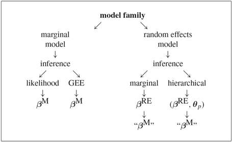
As an important example, consider our GLMM with logit link function, where the only random effects are intercepts bi. It can then be shown that the marginal mean μi=E(Yij) satisfies
h(μi)≈XiβM with
βREβM=√c2σ2+1>1,(5.27)
in which c equals 16√3/15π. Hence, although the parameters βRE in the generalized linear mixed model have no marginal interpretation, they do show a strong relation to their marginal counterparts. Note that, as a consequence of this relation, larger covariate effects are obtained under the random effects model in comparison to the marginal model.
After this longitudinal analysis, we can also restrict attention to the last planned occasion. However, the very nature of MAR implies that one still explicitly wants to consider the incomplete profiles for use in the correct estimation of effects when incompleteness occurs. Thus, one has to consider the full longitudinal model. The analyses considered before will therefore be the basis.
Let αi be the effect of treatment arm i at the last measurement occasion, where i can be A1 or C. We want to test whether at the last measurement occasion the effects of therapy A1 and the nonexperimental drug C are the same. This means αA1 = αC, or similarly αA1 – αC = 0. Using the parameter names as they are used in the SAS code (where C is the reference treatment), this translates to TRT. This hypothesis can easily be tested using the CONTRAST statement. The CONTRAST statement enables one to conduct a statistical test that several expressions simultaneously equal zero. The expressions are typically contrasts–that is, differences whose expected values equal zero under the hypothesis of interest. In the CONTRAST statement you must provide a quoted string to identify the contrast and then a list of valid SAS expressions separated by commas. Multiple CONTRAST statements are permitted, and results from all statements are listed in a common table. PROC NLMIXED constructs approximate F tests for each statement using the delta method to approximate the variance-covariance matrix of the constituent expressions.
In the NLMIXED procedure, we add only the following statement to Program 5.28:
contrast ’last visit’ trt;
Note that the same result is found by looking at the ouput of TRT in the “Parameter Estimates” section.
Output from Program 5.28 with CONTRAST statement added
Contrasts
| Label | Num DF |
Den DF |
F Value | Pr > F |
| last visit | 1 | 169 | 2.81 | 0.0954 |
Since p = 0.0954, we retain a nonsignificant result.
5.11 MNAR and Sensitivity Analysis
Even though the assumption of likelihood ignorability encompasses both MAR and the more stringent and often implausible MCAR mechanisms, it is difficult to exclude the option of a more general missingness mechanism. One solution is to fit an MNAR model as proposed by Diggle and Kenward (1994), who fitted models to the full data using the simplex algorithm (Nelder and Mead, 1965). However, as pointed out by several authors in discussion of Diggle and Kenward (1994), one has to be extremely careful with interpreting evidence for or against MNAR using only the data under analysis. See also Verbeke and Molenberghs (2000, Chapter 18).
A sensible compromise between blindly shifting to MNAR models or ignoring them altogether is to make them a component of a sensitivity analysis. In that sense, it is important to consider the effect on key parameters such as treatment effect or evolution over time. One such route for sensitivity analysis is to consider pattern-mixture models as a complement to selection models (Thijs et al., 2002; Michiels et al., 2002). Further routes to explore sensitivity are based on global and local influence methods (Verbeke et al., 2001; Molenberghs et al., 2001). Robins, Rotnitzky and Scharfstein (1998) discuss sensitivity analysis in a semiparametric context.
The same considerations can be made when compliance data are available. In such a case, arguably, a definitive analysis would not be possible and it might be sensible to resort to sensitivity analysis ideas (Cowles, Carlin and Connett, 1996).
A full treatment of sensitivity analysis is beyond the scope of this chapter.
5.12 Summary
We have indicated that analyzing incomplete (longitudinal) data, both of a Gaussian as well as of a non-Gaussian nature, can easily be conducted under the relatively relaxed assumption of missingness at random (MAR) using standard statistical software tools. Likelihood-based methods include the linear mixed model (e.g., implemented in the SAS procedure MIXED) and generalized linear mixed models (e.g., implemented in the SAS procedure NLMIXED). In addition, weighted generalized estimating equations (WGEE) can be used as a relatively straightforward alteration of ordinary generalized estimating equations (GEE) so that also this technique is valid under MAR. Both theoretical considerations as well as illustrations using two case studies have been given. These methods are highly useful when inferential focus is on the entire longitudinal profile or aspects thereof, as well as when one is interested in a single measurement occasion only, e.g., the last planned one.
Alternative methods which allow ignoring the missing data mechanism under MAR include multiple imputation (MI) and the expectation-maximization (EM) algorithm.
All of this implies that traditionally popular but much more restricted modes of analysis, including complete case (CC) analysis, last observation carried forward (LOCF), or other simple imputation methods, ought to be abandoned, given the highly restrictive assumptions on which they are based.