
Multiple Comparisons and Multiple Endpoints 2
2.4 Fixed-Sequence Testing Methods
2.5 Resampling-Based Testing Methods
2.6 Testing Procedures for Multiple Endpoints
This chapter discusses statistical strategies for handling multiplicity issues arising in clinical trials. It covers basic single-step multiple tests and more advanced closed, fixed-sequence and resampling-based multiple testing procedures. The chapter also reviews methods used in the analysis of multiple endpoints and gatekeeping testing strategies for clinical trials with multiple objectives and for dose-finding studies.
2.1 Introduction
Multiplicity problems arise in virtually every clinical trial. They are caused by multiple analyses performed on the same data. It is well known that performing multiple tests in a univariate manner by using unadjusted p-values increases the overall probability of false-positive outcomes. This problem is recognized by both drug developers and regulators. Regulatory agencies mandate a strict control of the overall Type I error rate in clinical trials because false positive trial findings could lead to approval of inefficacious drugs. The guidance document entitled “Points to consider on multiplicity issues in clinical trials” released by the European Committee for Proprietary Medicinal Products (CPMP) on September 19, 2002, emphasized the importance of addressing multiplicity issues in clinical trials by stating that
a clinical study that requires no adjustment of the Type I error is one that consists of two treatment groups, that uses a single primary variable, and has a confirmatory statistical strategy that prespecifies just one single null hypothesis relating to the primary variable and no interim analysis.
Along the same line, the ICH E9 guidance document on statistical principles for clinical trials states that
in confirmatory analyses, any aspects of multiplicity
… should be identified in the protocol; adjustment should always be considered and the details of any adjustment procedure … should be set out in the analysis plan.
There are several types of multiple testing problems encountered in clinical trials:
1. Multiple treatment comparisons. Most commonly, multiple testing is encountered in clinical trials involving several treatment groups. The majority of Phase II trials are designed to assess the efficacy and safety profile of several doses of an experimental drug compared to a placebo or an active control. Performing multiple comparisons of different dose levels of an experimental drug and a control causes multiplicity problems.
2. Multiple primary endpoints. Multiplicity is also caused by multiple criteria for assessing the efficacy or safety of an experimental drug. The multiple criteria are required to accurately characterize various aspects of the expected therapeutic benefits. For example, the efficacy profile of cardiovascular drugs is typically evaluated using multiple outcome variables such as all-cause mortality, nonfatal myocardial infarction, or refractory angina/urgent revascularization.
3. Multiple secondary analyses. It is commonly accepted that multiplicity issues in the primary analysis must be addressed in all efficacy trials; however, multiplicity adjustments are rarely performed with respect to secondary and subgroup analyses. Recent publications emphasize the need to carefully address these types of multiplicity issues in the trial protocol and to develop a hierarchy of analyses that includes the primary analysis and the most important secondary and subgroup analyses.
Overview
This chapter deals with statistical issues related to multiple comparisons and multiple endpoints in clinical trials. Sections 2.2 and 2.3 discuss single-step tests (e.g., Bonferroni test) and more powerful closed testing procedures such as the Holm and Hommel procedures. Section 2.4 covers fixed-sequence testing methods and Section 2.5 briefly reviews resampling-based methods for multiplicity adjustment with emphasis on clinical trial applications. See Hochberg and Tamhane (1987), Westfall and Young (1993) and Hsu (1996) for a more detailed discussion of issues related to multiple analyses. Westfall et al. (1999) and Westfall and Tobias (2000) provide an excellent overview of multiple comparison procedures with a large number of SAS examples.
Section 2.6 addresses multiplicity problems arising in clinical trials with multiple endpoints. There appears to be no monograph that provides a detailed coverage of statistical issues in the analysis of multiple clinical endpoints. The interested reader is referred to review papers by Pocock, Geller and Tsiatis (1987), Lee (1994) and Wassmer et al. (1999).
Finally, Section 2.7 discusses multiple testing procedures for families of hypotheses with a sequential structure. Sequential families are encountered in clinical trials with multiple objectives (based on primary, secondary and possibly tertiary endpoints) and in dose-finding studies. For a summary of recent research in this area, see Westfall and Krishen (2001) and Dmitrienko, Offen and Westfall (2003).
Weak and Strong Control of Familywise Error Rate
To control the overall error rate in situations involving multiple testing, the statistician needs to answer the billion-dollar question (the billion-dollar part is not an exaggeration in the context of modern drug development!):
How does one define the family of null hypotheses to be tested and the incorrect decisions whose likelihood needs to be controlled?
In most cases, the family of hypotheses is defined at the trial level. This means that all multiple analyses are to be performed in such a way that the trialwise error rate is maintained at the prespecified level.
Further, there are two definitions of the overall (familywise) error rate. We need to understand what inferences we intend to perform in order to choose the right definition of the overall error rate and an appropriate multiple testing method. To illustrate, consider the following example that will be used throughout Sections 2.2 and 2.3.
EXAMPLE: Dose-Finding Hypertension Trial
Suppose that a dose-finding trial has been conducted to compare low, medium and high doses of a new antihypertensive drug (labeled L, M and H) to a placebo (labeled P). The primary efficacy variable is diastolic blood pressure. Doses that provide a clinically relevant mean reduction in diastolic blood pressure will be declared efficacious.
Let μP denote the mean reduction in diastolic blood pressure in the placebo group. Similarly, μL, μM and μH denote the mean reduction in diastolic blood pressure in the low, medium and high dose groups, respectively. The null hypothesis of equality of μP, μL, μM and μH (known as the global null hypothesis) can be tested in the hypertension trial example using the usual F-test. The F-test is said to preserve the overall Type I error rate in the weak sense, which means that it controls the likelihood of rejecting the global null hypothesis when all individual hypotheses are simultaneously true.
The weak control of the familywise error rate is appropriate only if we want to make a statement about the global null hypothesis. In order to test the effects of the individual doses on diastolic blood pressure, we need to control the probability of erroneously rejecting any true null hypothesis regardless of which and how many null hypotheses are true. This is referred to as the strong control of the familywise error rate. For example, the procedure proposed by Dunnett (1955) can be used to test the global null hypothesis and, at the same time, to provide information about individual dose-placebo comparisons (e.g., μP versus μL, μP versus μM and μP versus μH). This procedure controls the familywise error rate in the strong sense. Given the importance of the strong control of Type I outcomes in clinical applications, this chapter will focus only on methods that preserve the familywise error rate in the strong sense.
It is worth noting that there are other definitions of the likelihood of an incorrect decision, such as the false discovery rate introduced by Benjamini and Hochberg (1995). Multiple tests controlling the false discovery rate are more powerful (and more liberal) than tests designed to protect the familywise error rate in the strong sense and are useful in multiplicity problems with a large number of null hypotheses. False discovery rate methods are widely used in preclinical research (e.g., genetics) and have recently been applied to the analysis of clinical trial data. Mehrotra and Heyse (2001) used the false discovery rate methodology to develop an efficient strategy for handling multiplicity issues in the evaluation of safety endpoints. Another interesting strategy is to employ Bayesian methods in multiplicity adjustments. Bayesian approaches to multiple testing with clinical trial applications have been investigated in several publications; see, for example, Westfall et al. (1999, Chapter 13) and Gönen, Westfall and Johnson (2003).
Multiple Tests Based on Marginal p-Values
Sections 2.2 and 2.3 deal with popular multiple tests based on marginal p-values. These tests can be thought of as “distribution-free” tests because they rely on elementary probability inequalities and thus do not depend on the joint distribution of test statistics. Marginal multiple testing procedures are intuitive and easy to apply. These procedures offer a simple way to “fix” Type I error inflation problems in any situation involving multiple testing—e.g., in clinical trials with multiple treatment comparisons, multiple endpoints or interim analyses. Therefore, it should not be surprising that tests based on marginal p-values enjoy much popularity in clinical applications (Chi, 1998).
The obvious downside of marginal tests is that they rely on the marginal distribution of individual test statistics and ignore the underlying correlation structure. As a result, multiple tests that make full use of the joint distribution of test statistics outperform marginal tests, especially when the test statistics are highly correlated or the number of multiple analyses is large.
2.2 Single-Step Tests
There are two important classes of multiple testing procedures that will be considered in this and subsequent sections: single-step and stepwise tests. Both single-step and stepwise tests fall in a very broad class of closed testing procedures that will be reviewed in Section 2.3. Single-step methods (e.g., the Bonferroni method) test each null hypothesis of interest independently of the other hypotheses. In other words, the order in which the null hypotheses are examined is not important and the multiple inferences can be thought of as being performed in a single step. In contrast, stepwise testing procedures (e.g., the Holm stepwise procedure) test one hypothesis at a time in a sequential manner. As a result, some of the null hypotheses may not be tested at all. They may be either retained or rejected by implication. Stepwise procedures are superior to simple single-step tests in the sense that they increase the number of rejected null hypotheses without inflating the familywise error rate.
Suppose we plan to carry out m significance tests corresponding to a family of null hypotheses denoted by H1,…, Hm. The global null hypothesis is defined as the intersection of H1,…, Hm, i.e.,
{H1 and H2 and … and Hm}
Let p1,…, pm denote the individual p-values generated by the significance tests. The ordered p-values p(1),…,p(m) are defined in such a way that
p(1)≤p(2)≤…≤p(m).
We wish to devise a simultaneous test for the family of null hypotheses. The test will be based on a suitable adjustment for multiplicity to keep the familywise error rate at the prespecified α level. Multiplicity adjustments are performed by modifying the individual decision rules—i.e., by adjusting either the individual p-values or significance levels (p-values are adjusted upward or significance levels are adjusted downward). To define adjusted p-values, we adopt the definition proposed by Westfall and Young (1993). According to this definition, the adjusted p-value equals the smallest significance level for which one would reject the corresponding null hypothesis.
There are three popular multiplicity adjustment methods (the Bonferroni, Šidák and Simes methods) that underlie the majority of multiple testing procedures based on marginal p-values. The methods are briefly discussed below.
Bonferroni and Šidák Methods
The Bonferroni and Šidák methods are perhaps the most widely used multiplicity adjustments. These methods are available in a large number of SAS procedures, such as PROC GLM, PROC MIXED, and PROC MULTTEST. Their implementation is very straightforward. The Bonferroni multiple test rejects Hi if pi ≤ α/m, and the Šidák multiple test rejects Hi if pi ≤ 1 – (1 — α)1/m, where i = 1,…,m. The individual adjusted p-values for the two tests are given by
˜pi=mpi(Bonferroni), ˜pi=1−(1−pi)m
Using the Bonferroni inequality, it is easy to show that the Bonferroni multiple test controls the familywise error rate in the strong sense for any joint distribution of the raw p-values. However, the Šidák multiple test does not always preserve the familywise error rate. Šidák (1967) demonstrated that the size of this test does not exceed α when the individual test statistics are either independent or follow a multivariate normal distribution. Holland and Copenhaver (1987) described a broad set of assumptions under which the Šidák test controls the familywise error rate—for example, when the test statistics follow t and some other distributions.
The Bonferroni and Šidák tests can also be used to test the global null hypothesis. The global hypothesis is rejected whenever any of the individual null hypotheses is rejected. This means that the Bonferroni global test rejects the global hypothesis if pi ≤ α/m for at least one i = 1,…, m. Likewise, the Šidák global test rejects the global hypothesis if pi ≤ 1 – (1 — α)1/mfor at least one i = 1,…, m.
The adjusted p-values associated with the Bonferroni and Šidák global tests are given by
˜PB=m min(p1,…,pm)(Bonferroni),
˜PS=1−(1−min(p1,…,pm))m
In other words, the Bonferroni and Šidák global tests reject the global null hypothesis if ˜PB≤α
It is easy to show that the Šidák correction is uniformly better than the Bonferroni correction (Hsu, 1996, Section 1.3.5). The difference between these two corrections is rather small when the raw p-values are small. The two tests are known to be very conservative when the individual test statistics are highly correlated. The adjusted p-values generated by the Bonferroni and Šidák procedures are considerably larger than they need to be to maintain the familywise error rate at the desired level.
To illustrate the Bonferroni and Šidák adjustments (as well as other multiple tests that will be discussed later in this section), consider the dose-finding hypertension trial example. Recall that μP denotes the mean reduction in diastolic blood pressure in the placebo group and μL, μM and μH denote the mean reduction in diastolic blood pressure in the low, medium and high dose groups, respectively. Negative values of μL, μM and μH indicate an improvement in diastolic blood pressure. The following null hypotheses are tested in the trial:
HL={μP−μL≤δ}, HM={μP−μM≤δ}, HH={μP−μH≤δ},
where δ represents a clinically significant improvement over placebo. The treatment means are compared using the two-sample t-test. Table 2.1 shows p-values generated by the three dose-placebo comparisons under three scenarios.
Table 2.1 Dose-placebo comparisons in hypertension trial
| Comparison | L vs. P | M vs. P | H vs. P |
| Scenario 1 | pL = 0.047 | pM = 0.0167 | pH = 0.015 |
| Scenario 2 | pL = 0.047 | pM = 0.027 | pH = 0.015 |
| Scenario 3 | pL = 0.053 | pM = 0.026 | pH = 0.017 |
Program 2.1 computes adjusted p-values produced by the Bonferroni and Šidák tests under Scenario 1. The two tests are requested by the BONFERRONI and SIDAK options in PROC MULTTEST.
Program 2.1 Analysis of the hypertension trial using the Bonferroni and Šidák tests
data antihyp1;
input test $ raw_p @@;
datalines;
L 0.047 M 0.0167 H 0.015
;
proc multtest pdata=antihyp1 bonferroni sidak out=adjp;
axis1 minor=none order=(0 to 0.15 by 0.05) label=(angle=90 "P-value");
axis2 minor=none value=("Low" "Medium" "High") label=("Dose")
order=("L" "M" "H");
symbol1 value=circle color=black i=j;
symbol2 value=diamond color=black i=j;
symbol3 value=triangle color=black i=j;
proc gplot data=adjp;
plot raw_p*test bon_p*test sid_p*test/frame overlay nolegend
haxis=axis2 vaxis=axis1 vref=0.05 lvref=34;
run;
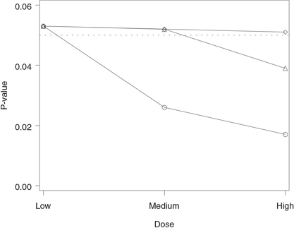
Figure 2.1 Analysis of the hypertension trial using the Bonferroni and Šidák tests. Raw p-value (○), Bonferroni-adjusted p-value (◇) and Šidák-adjusted p-value (△).
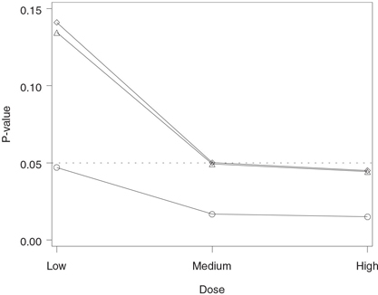
The output of Program 2.1 is shown in Figure 2.1. The figure displays the adjusted p-values produced by the Bonferroni and Šidák tests plotted along with the corresponding raw p-values. The figure indicates that the raw p-values associated with all three dose-placebo comparisons are significant at the 5% level, yet only the high dose is significantly different from placebo after the Bonferroni adjustment for multiplicity (p = 0.045). The Šidák-adjusted p-values are consistently less than the Bonferroni-adjusted p-values; however, the difference is very small. The Šidák-adjusted p-value for the medium dose versus placebo comparison is marginally significant (p = 0.0493), whereas the corresponding Bonferroni-adjusted p-value is only a notch greater than 0.05 (p = 0.0501).
Despite the conservative nature of the Bonferroni adjustment, it has been shown in the literature that the Bonferroni method cannot be improved (Hommel, 1983). One can find fairly exotic p-value distributions for which the Bonferroni inequality turns into an equality and therefore it is impossible to construct a single-step test that will be uniformly more powerful than the simple Bonferroni test. The only way to improve the Bonferroni method is by making additional assumptions about the joint distribution of the individual p-values. Examples of multiple tests that rely on the assumption of independent p-values will be given in the next subsection.
Simes Method
Unlike the Bonferroni and Šidák methods, the Simes method can be used only for testing the global null hypothesis. We will show in Section 2.3 that the Simes global test can be extended to perform inferences on individual null hypotheses, and we will demonstrate how to carry out the extended tests using PROC MULTTEST.
The Simes method is closely related to that proposed by Rüger (1978). Rüger noted that the Bonferroni global test can be written as
Reject the global null hypothesis {H1 and H2 and … and Hm} if p(1) ≤ α/m
and uses only a limited amount of information from the sample. It relies on the most significant p-value and ignores the rest of the p-values. Rüger described a family of generalized Bonferroni global tests based on the ordered p-values p(1),…,p(m). He showed that the global null hypothesis can be tested using any of the following tests:
p(1)≤α/m, p(2)≤2α/m, p(3)≤3α/m, …, p(m)≤α.
For example, one can test the global null hypothesis by comparing p(2) to 2α/m or p(3) to 3α/m as long as one prespecifies which one of these tests will be used. Any one of Rüger’s global tests controls the Type I error rate in the strong sense for arbitrary dependence structures. However, each test suffers from the same problem as the Bonferroni global test: each individual test is based on only one p-value.
Simes (1986) developed a procedure for combining the information from m individual tests. The Simes global test rejects the global null hypothesis if
p(i)≤iα/m for at least one i=1,…,m.
Simes demonstrated that his global test is exact in the sense that its size equals α if p1,…, pm are independent. The adjusted p-value for the global hypothesis associated with this test is equal to
˜pSIM=m min(p(1)/1,p(2)/2,…,p(m)/m).
Since ˜pB=mp(1),
The Simes test achieves higher power by assuming that the individual p-values are independent. Naturally, this assumption is rarely satisfied in clinical applications. What happens if the p-values are correlated? In general, the Simes global test does not preserve the Type I error rate. Hommel (1983) showed that the Type I error rate associated with the Simes test can be considerably higher than α. In fact, it can be as high as
(1+12+…+1m)α,
i.e., 1.5α if m = 2 and 2.08α if m = 4.
The case of independent p-values often represents the worst-case scenario in terms of the amount of Type I error rate inflation. For example, Simes (1986) showed via simulations that the Type I error rate associated with his test decreases with increasing correlation coefficient when the test statistics follow a multivariate normal distribution. Hochberg and Rom (1995) reported the results of a simulation study based on negatively correlated normal variables in which the size of the Simes test was close to the nominal value. Sarkar and Chang (1997) studied the Simes global test and demonstrated that it preserves the Type I error rate when the joint distribution of the test statistics exhibits a certain type of positive dependence. For example, multiple testing procedures based on the Simes test control the familywise error rate in the problem of performing multiple treatment-control comparisons under normal assumptions.
2.2.1 Summary
This section described simple multiplicity adjustment strategies known as single-step methods. Single-step procedures test each null hypothesis of interest independently of the other hypotheses and therefore the order in which the null hypotheses are examined becomes unimportant. Single-step tests are very easy to implement and have enjoyed much popularity in clinical applications.
The following three single-step tests were discussed in the section:
• The Bonferroni test controls the familywise error rate for any joint distribution of the marginal p-values but is known to be rather conservative. Despite the conservative nature of the Bonferroni method, no single-step test is uniformly more powerful than the Bonferroni test. More powerful tests can be constructed only if one is willing to make additional assumptions about the joint distribution of p-values associated with the null hypotheses of interest.
• The Šidák test is uniformly more powerful than the Bonferroni test; however, its size depends on the joint distribution of the marginal p-values and can exceed the nominal level. The Šidák test controls the familywise error rate when the test statistics are independent or follow a multivariate normal distribution.
• The Simes test can be used only for testing the global null hypothesis. The Simes global test is more powerful than the Bonferroni global test but does not always preserve the Type I error rate. Its size is known to be no greater than the nominal level when the individual test statistics are independent or positively dependent in the sense of Sarkar and Chang (1997).
Multiplicity adjustments based on the Bonferroni and Šidák tests are implemented in PROC MULTTEST and are also available in other SAS procedures, such as PROC GLM and PROC MIXED.
2.3 Closed Testing Methods
The closed testing principle was formulated by Marcus, Peritz and Gabriel (1976) and has since provided mathematical foundation for numerous multiple testing methods. It would not be an exaggeration to say that virtually all multiple testing procedures are either derived using this principle or can be rewritten as closed testing procedures. In fact, Liu (1996) showed that any single-step or stepwise multiple test based on marginal p-values can be formulated as a closed testing procedure. This means that one can always construct a closed testing procedure that is at least as powerful as any single-step or stepwise test.
The principle provides statisticians with a very powerful tool for addressing multiplicity problems in numerous settings. Bauer (1991) described a variety of closed testing procedures with applications to multiple comparisons, multivariate endpoints and repeated significance testing. Rom, Costello and Connell (1994) discussed the problem of testing a dose-response effect in dose-finding trials using a closed testing approach. Koch and Gansky (1996) and Chi (1998) reviewed applications of closed testing procedures in the context of clinical trials including multiple treatment comparisons and multiple subgroup analyses. The only major disadvantage of closed testing procedures is that it is generally difficult, if not impossible, to construct associated simultaneous confidence intervals for parameters of interest.
The closed testing principle is based on a hierarchical representation of a multiplicity problem. As an illustration, consider the three null hypotheses HL, HM and HH tested in the dose-finding hypertension trial introduced earlier in this section. To apply the closed testing principle to this multiple testing problem, we need to construct what is known as the closed family of hypotheses associated with the three original hypotheses. This is accomplished by forming all possible intersections of HL, HM and HH. The closed family will contain the following seven intersection hypotheses:
1. Three original hypotheses, HL, HM and HH.
2. Three intersection hypotheses containing two original hypotheses, {HL and HM}, {HL and HH} and {HM and HH}.
3. One intersection hypothesis containing three original hypotheses, {HL and HM and HH}.
The next step is to link the intersection hypotheses. The links are referred to as implication relationships. A hypothesis that contains another hypothesis is said to imply it. For example,
{HL and HM and HH}
implies {HL and HM}, which in turn implies HL. Most commonly, implication relationships are displayed using diagrams similar to that shown in Figure 2.2. Each box in this figure represents a hypothesis in the closed family and is connected to the boxes corresponding to the hypotheses it contains. Note that HLMH denotes the intersection hypothesis {HL and HM and HH}, HLM denotes the intersection hypothesis {HL and HM}, and so on. The hypothesis at the top is the intersection of the three original hypotheses and therefore it implies HLM, HLH and HMH. Likewise, the three boxes at the second level are connected to the boxes representing the original hypotheses HL, HM and HH. Alternatively, we can put together a list of all intersection hypotheses in the closed family implying the three original hypotheses (Table 2.2).
Figure 2.2 Implication relationships in the closed family of null hypotheses from the hypertension trial. Each box in this diagram represents a hypothesis in the closed family and is connected to the boxes corresponding to the hypotheses it implies.
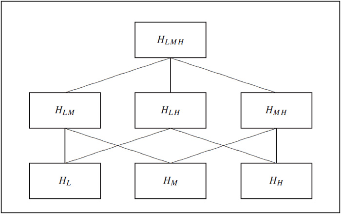
Table 2.2 Intersection hypotheses implying the original hypotheses
| Original hypothesis | Intersection hypotheses implying the original hypothesis |
| HL | HL, HLM, HLH, HLMH |
| HM | HM, HLM, HMH, HLMH |
| HH | HH, HLH, HMH, HLMH |
Closed Testing Principle
The closed testing principle states that one can control the familywise error rate by using the following multiple testing procedure:
Test each hypothesis in the closed family using a suitable α-level significance test that controls the error rate at the hypothesis level. A hypothesis is rejected if its associated test and all tests associated with hypotheses implying it are significant.
According to the closed testing principle, to reject any of the original hypotheses in the left column of Table 2.2, we need to test and reject all associated intersection hypotheses shown in the right column. If any one of the intersection hypotheses is retained then all hypotheses implied by it must also be retained by implication without testing.
Any valid significance test can be used to test intersection hypotheses in the closed family as long as its size does not exceed α at the hypothesis level. One can carry out the global F-test if the individual test statistics are independent or the Bonferroni global test if they are not. Each of these tests will result in a different closed testing procedure. However, as shown by Marcus, Peritz and Gabriel (1976), any multiple test based on the closed testing principle controls the familywise error rate in the strong sense at the prespecified α level.
2.3.1 Stepwise Closed Testing Methods
The reason the closed testing principle has become so popular is that it can be used to construct powerful multiple testing procedures. Consider, for example, the null hypotheses tested in the dose-finding hypertension trial. Choose a single-step test that controls the error rate at the hypothesis level and begin with the global hypothesis HLMH. If the associated test is not significant, we retain the global hypothesis and, according to the closed testing principle, we must retain all other hypotheses in the closed family, including HL, HM and HH. Otherwise, we go on to test the intersection hypotheses HLM, HLH and HMH. If any one of these hypotheses is rejected, we test the hypotheses implied by it and so on. Once we stop, we need to examine the implication relationships to see which of the original hypotheses can be rejected. The obtained closed procedure is more powerful than the single-step test it is based on.
Holm Stepwise Test
In certain cases, the described hierarchical testing algorithm can be significantly simplified. In those cases, the significance testing can be carried out in a straightforward stepwise manner without examining all implication relationships. As an illustration, suppose we wish to enhance the Bonferroni correction by utilizing the closed testing principle. It is a well-known fact that applying the closed testing principle with the Bonferroni global test yields the Bonferroni stepwise procedure introduced by Holm (1979); see Hochberg and Tamhane (1987, Section 2.4).
Choose an arbitrary intersection hypothesis H in the closed family (see Table 2.2). The hypothesis will be tested using the Bonferroni global test; i.e., the following decision rule will be employed:
Compute the p-value associated with the Bonferroni global test. The p-value is equal to the most significant p-value corresponding to the original hypotheses implied by H times the number of original hypotheses implied by H. Denote the obtained p-value by ˜pB
For example, consider the intersection hypothesis HLM. This intersection hypothesis implies two original hypotheses, namely, HL and HM. Therefore, the Bonferroni-adjusted p-value is given by ˜pB=2min(pL,pM)
By the Bonferroni inequality, the size of the Bonferroni global test is no greater than α. This means that we have constructed a family of α-level significance tests for each hypothesis in the closed family. Therefore, applying the closed testing principle yields a multiple test for the original hypotheses HL, HM and HH that protects the overall Type I error rate in the strong sense.
The constructed multiple test looks fairly unwieldy at first glance. Despite this first impression, it has a simple stepwise form. Consider a general family of null hypotheses H1,…,Hm. The Holm multiple test is based on a sequentially rejective algorithm that tests the ordered hypotheses H(1),…,H(m) corresponding to the ordered p-values p(1),…,p(m). The multiple testing procedure begins with the hypothesis associated with the most significant p-value, i.e., with H(1). This hypothesis is rejected if p(1) ≤ α/m. Further, H(i) is rejected at the ith step if p(j) ≤ α/(m – j + 1) for all j = 1,…,i. Otherwise, H(i),…,H(m) are retained and the algorithm terminates. The details of the Holm test are shown in Table 2.3.
To compare the Holm and Bonferroni testing procedures, note that the Bonferroni procedure tests H1,…, Hm at the same α/m level. In contrast, the Holm procedure tests H(1) at the α/m level and the other hypotheses are tested at successively higher significance levels. As a result, the Holm stepwise test rejects at least as many (and possibly more) hypotheses as the Bonferroni test. This means that, by applying the closed testing principle, we have constructed a more powerful test that maintains the familywise error rate at the same level.
Table 2.3 Holm stepwise test
| Step | Condition | Condition is met | Condition is not met |
| 1 | p(1) ≤ α/m | Reject H(1) and go to Step 2 |
Retain H(1),…,H(m) and stop |
| … | … | … | … |
| i | p(i) ≤ α/(m – i + 1) | Reject H(i) and go to Step i + 1 |
Retain H(i),…,H(m) and stop |
| … | … | … | … |
| m | p(m) ≤ α | Reject H(m) | Retain H(m) |
To illustrate this important feature of the Holm stepwise procedure, consider Scenario 1 in Table 2.1. Program 2.2 shows how to compute adjusted p-values produced by the Bonferroni and Holm multiple tests using PROC MULTTEST. The Bonferroni and Holm tests are requested by the BONFERRONI and STEPBON options.
Program 2.2 Analysis of the hypertension trial using the Bonferroni and Holm tests
proc multtest pdata=antihyp1 bonferroni stepbon out=adjp;
axis1 minor=none order=(0 to 0.15 by 0.05) label=(angle=90 "P-value");
axis2 minor=none value=("Low" "Medium" "High") label=("Dose")
order=("L" "M" "H");
symbol1 value=circle color=black i=j;
symbol2 value=diamond color=black i=j;
symbol3 value=triangle color=black i=j;
proc gplot data=adjp;
plot raw_p*test bon_p*test stpbon_p*test/frame overlay nolegend
haxis=axis2 vaxis=axis1 vref=0.05 lvref=34;
run;
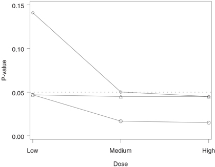
The output of Program 2.2 is displayed in Figure 2.3. Figure 2.3 shows that all three Holm-adjusted p-values are less than 0.05 (note that the adjusted p-value for the low dose versus placebo comparison is equal to the corresponding raw p-value). This means that the Holm stepwise procedure has rejected all three null hypotheses, indicating that all doses of the experimental drug provide a significantly greater reduction in diastolic blood pressure compared to the placebo. In contrast, only the high dose is significantly different from the placebo according to the Bonferroni correction.
2.3.2 Decision Matrix Algorithm
Only a limited number of closed testing procedures have a simple stepwise representation similar to that of the Holm multiple test. Most of the time, the statistician does not have the luxury of being able to set up a stepwise algorithm and needs to carefully review the complex implication relationships to ensure the closed testing principle is applied properly and the familywise error rate is not inflated. Due to the hierarchical nature of closed testing procedures, this can be a challenging task when a large number of hypotheses are being tested.
In this subsection we will introduce the decision matrix algorithm for implementing general closed testing procedures. This algorithm streamlines the decision-making process and simplifies the computation of adjusted p-values associated with the intersection and original hypotheses; see Dmitrienko, Offen and Westfall (2003) for details and examples. To illustrate the decision matrix method, we will show how it can be used to carry out the Holm stepwise test. The method will also be
Figure 2.3 Analysis of the hypertension trial using the Bonferroni and Holm tests. Raw p-value (○), Bonferroni-adjusted p-value (◇) and Holm-adjusted p-value (△).
applied to construct closed testing procedures for the" identification of individual significant outcomes in clinical trials with multiple endpoints in Section 2.6 and for setting up gatekeeping procedures in Section 2.7.
Holm Stepwise Test
Consider the null hypotheses tested in the dose-finding hypertension trial. Table 2.4 presents a decision matrix for the Holm multiple test. It summarizes the algorithm for computing the adjusted p-values that are later used in testing the significance of individual dose-placebo comparisons.
Table 2.4 Decision matrix for the Holm multiple test
| Implied hypotheses | ||||
| Intersection hypothesis |
p-value | HL | HM | HH |
| HLMH | pLMH = 3 min(pL, pM, pH) | pLMH | pLMH | pLMH |
| HLM | pLM = 2 min(pL, pM | pLM | pLM | 0 |
| HLH | pLH = 2 min(pL, pH | pLH | 0 | PLH |
| HL | pL = pL | pL | 0 | 0 |
| HMH | pMH = 2 min(pM, pH) | 0 | pM | 0 |
| HH | pH = pH) | 0 | 0 | pH |
There are seven rows in Table 2.4, each corresponding to a single intersection hypothesis in the closed family. For each of these hypotheses, the three columns on the right side of the table" identify the implied hypotheses, while the second column displays the formula for computing the associated p-values denoted by
pLMH, pLM, pLH, pMH, pL, pM, pH.
In order to make inferences about the three original hypotheses, we first compute these p-values and populate the three columns on the right side of the table. Westfall and Young (1993) stated that the adjusted p-value for each original hypothesis is equal to the largest p-value associated with the intersection hypotheses that imply it. This means that we can obtain the adjusted p-values for HL, HM and HH by computing the largest p-value in the corresponding column on the right side of the table. For example, the adjusted p-value for the low dose versus placebo comparison is equal to
max(pL, pLM, pLH, pLMH)
Program 2.3 computes the Holm-adjusted p-values using the decision matrix algorithm.
Program 2.3 Analysis of the hypertension trial using the Holm multiple test (decision matrix approach)
proc iml;
use antihyp1;
read all var {raw_p} into p;
h=j(7,3,0);
decision_matrix=j(7,3,0);
adjusted_p=j(1,3,0);
do i=1 to 3;
do j=0 to 6;
k=floor(j/2**(3-i));
if k/2=floor(k/2) h[j+1,i]=1;
end;
end;
do i=1 to 7;
decision_matrix[i,]=h[i,]*sum(h[i,])*min(p[loc(h[i,])]);
end;
do i=1 to 3;
adjusted_p[i]=max(decision_matrix[,i]);
end;
title={"L vs P", "M vs P", "H vs P"};
print decision_matrix[colname=title];
print adjusted_p[colname=title];
quit;
Output from Program 2.3
DECISION_MATRIX
| L vs P | M vs P | H vs P |
| 0.045 | 0.045 | 0.045 |
| 0.0334 | 0.0334 | 0 |
| 0.03 | 0 | 0.03 |
| 0.047 | 0 | 0 |
| 0 | 0.03 | 0.03 |
| 0 | 0.0167 | 0 |
| 0 | 0 | 0.015 |
| ADJUSTED_P | ||
| L vs P | M vs P | H vs P |
| 0.047 | 0.045 | 0.045 |
The DECISION MATRIX table in Output 2.3 represents the three columns on the right of Table 2.4 and serves as a helpful tool for visualizing the decision-making process behind the closed testing procedure. As was noted earlier, the adjusted p-values for HL, HM and HH can be obtained by computing the maximum over all p-values in the corresponding column. The computed p-values are shown at the bottom of Output 2.3. Note that these adjusted p-values are" identical to those produced by PROC MULTTEST in Program 2.2.
2.3.3 Popular Closed Testing Procedures
It was shown in the previous subsection that one can significantly improve the performance of the Bonferroni correction by constructing a closed testing procedure based on the Bonferroni global test (i.e., the Holm procedure). The same" idea can be used to enhance any single-step test for the global null hypothesis described in Section 2.2, such as the Šidák or Simes global test. While no one appears to have taken credit for developing a closed testing procedure based on the Šidák global test, several authors have proposed closed testing procedures derived from the Bonferroni and Simes global tests. We will briefly review multiple tests developed by Shaffer (1986), Hommel (1988) and Hochberg (1988).
All of the multiple tests discussed in this subsection are superior to the Holm procedure in terms of power. However, it is important to remember that the Holm procedure is based on the Bonferroni global test, which cannot be sharpened unless additional assumptions about the joint distributions of p-values are made. This means that one needs to pay a price to improve the Holm test. Some of the multiple tests described below are efficient only for certain types of multiple testing problems and some of them lose the strict control of the overall Type I error rate.
Shaffer Multiple Test
Shaffer (1986) proposed an enhanced version of the stepwise Bonferroni procedure by assuming that the hypotheses of interest are linked to each other; i.e., a rejection of one hypothesis immediately implies that another one is rejected. The Shaffer method is highly efficient in multiple testing problems involving a large number of pairwise comparisons, such as dose-finding studies. When the hypotheses being tested are not logically interrelated (e.g., when multiple comparisons with a control are performed), the Shaffer procedure reduces to the Holm procedure.
Hommel Multiple Test
A closed testing procedure based on the Simes test was proposed by Hommel (1986, 1988). Unlike the Simes test, which can be used only for testing the global null hypothesis, the Hommel testing procedure starts with the global hypothesis and then “steps down” to examine the individual hypotheses. Since the Simes global test is more powerful than the Bonferroni global test, the Hommel procedure rejects all hypotheses rejected by the Holm closed procedure based on the Bonferroni procedure, and possibly more. However, the improvement comes with a price. The Hommel test no longer guarantees that the probability of an overall Type I error is at most α. The Hommel procedure protects the familywise error rate only when the Simes global test does—e.g., when the individual test statistics are independent or positively dependent (Sarkar and Chang, 1997).
Unlike the Holm multiple test, the Hommel test cannot be carried out in a simple sequentially rejective manner. The test can be implemented using the decision matrix algorithm and one can write a SAS program similar to Program 2.3 to compute the Hommel-adjusted p-values for HL, HM and HH. Here, we will present an efficient solution that utilizes PROC MULTTEST. The Hommel multiple test is available in PROC MULTTEST in SAS 8.1 and later versions of the SAS System. It can be requested using the HOMMEL option. PROC MULTTEST produces the same adjusted p-values as the decision matrix approach.
Program 2.4 computes the Holm- and Hommel-adjusted p-values for the individual dose-placebo comparisons in the hypertension trial under Scenario 2 shown in Table 2.1.
Program 2.4 Analysis of the hypertension trial using the Holm and Hommel tests
data antihyp2;
input test $ raw_p @@;
datalines;
L 0.047 M 0.027 H 0.015
;
proc multtest pdata=antihyp2 stepbon hommel out=adjp;
axis1 minor=none order=(0 to 0.06 by 0.02) label=(angle=90 "P-value");
axis2 minor=none value=("Low" "Medium" "High") label=("Dose")
order=("L" "M" "H");
symbol1 value=circle color=black i=j;
symbol2 value=diamond color=black i=j;
symbol3 value=triangle color=black i=j;
proc gplot data=adjp;
plot raw_p*test stpbon_p*test hom_p*test/frame overlay nolegend
haxis=axis2 vaxis=axis1 vref=0.05 lvref=34;
run;
Figure 2.4 Analysis of the hypertension trial using the Holm and Hommel tests. Raw p-value (◯), Holm-adjusted p-value (◇) and Hommel-adjusted p-value (△).
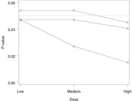
The output of Program 2.4 is displayed in Figure 2.4. The figure demonstrates that the Hommel testing procedure has rejected all three null hypotheses and thus it is clearly more powerful than the Holm procedure, which rejected only one hypothesis (note that the Hommel-adjusted p-value for the low dose versus placebo comparison is equal to the corresponding raw p-value). The figure also illustrates an interesting property of the Hommel procedure. Since the Hommel procedure is based on the Simes test, it rejects all null hypotheses whenever all raw p-values are significant.
Hochberg Multiple Test
Another popular stepwise test supported by PROC MULTTEST is the Hochberg test (Hochberg, 1988). This test is virtually" identical to the Holm test except for the order in which the null hypotheses are tested. As was explained earlier, the Holm multiple test examines the most significant p-value first and then works downward. For this reason, it is commonly referred to as a step-down test. In contrast, the Hochberg procedure examines the ordered p-values p(1),…, p(m) starting with the largest one and thus falls into the class of step-up tests.
The Hochberg multiple test rejects all hypotheses rejected by the Holm test but is uniformly less powerful than the Hommel procedure (Hommel, 1989). Also, like the Hommel test, the Hochberg test does not always preserve the familywise error rate. Its size can potentially exceed α but it is no greater than α when the individual p-values are independent. This means that in all situations when both of these tests can be carried out, the Hommel multiple test should be given a preference.
The Hochberg procedure is available in MULTTEST and can be requested using the HOCHBERG option. Program 2.5 computes the Hochberg- and Hommel-adjusted p-values for the three null hypotheses tested in the dose-finding hypertension trial under Scenario 3 shown in Table 2.1.
Program 2.5 Analysis of the hypertension trial using the Hochberg and Hommel tests
data antihyp3;
input test $ raw_p @@;
datalines;
L 0.053 M 0.026 H 0.017
;
proc multtest pdata=antihyp2 hochberg hommel out=adjp;
axis1 minor=none order=(0 to 0.06 by 0.02) label=(angle=90 "P-value");
axis2 minor=none value=("Low" "Medium" "High") label=("Dose")
order=("L" "M" "H");
symbol1 value=circle color=black i=j;
symbol2 value=diamond color=black i=j;
symbol3 value=triangle color=black i=j;
proc gplot data=adjp;
plot raw_p*test hoc_p*test hom_p*test/frame overlay nolegend
haxis=axis2 vaxis=axis1 vref=0.05 lvref=34;
run;
Figure 2.5 Analysis of the hypertension trial using the Hochberg and Hommel tests. Raw p-value (◯), Hochberg-adjusted p-value (◇) and Hommel-adjusted p-value (△).
The output of Program 2.5 is shown in Figure 2.5. We can see from Figure 2.5 that the Hommel multiple test has rejected more null hypotheses than the Hochberg test. Note that both the Hochberg-and Hommel-adjusted p-values for the low dose versus placebo comparison are equal to the corresponding raw p-value.
Power Comparisons
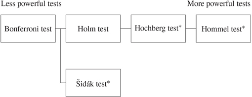
Figure 2.6 displays the relationship among the two single-step and three stepwise multiple tests discussed in this and previous sections. The multiple tests shown in Figure 2.6 are arranged in the order of increasing power. The tests on the right-hand side are uniformly more powerful than the tests on the left-hand side. Although the testing procedures derived from the Simes and related multiple tests (i.e., Hochberg and Hommel procedures) are more powerful than the Holm and Bonferroni tests, one needs to remember that these procedures do not always control the familywise error rate. The familywise error rate is protected if the individual test statistics are independent or positively dependent (Sarkar and Chang, 1997).
Figure 2.6 A comparison of five popular multiple tests. Tests displayed on the right-hand side are uniformly more powerful than tests on the left-hand side. An asterisk indicates that the test does not always control the familywise error rate.
A number of authors investigated the Type I and Type II error rates associated with popular multiple tests. Dunnett and Tamhane (1992) performed a simulation study to compare several stepwise procedures in the context of multiple treatment-control tests under normal theory. Dunnett and Tamhane observed marginal increases in power when they compared the Hommel procedure with the Holm procedure.
Brown and Russell (1997) reported the results of an extensive simulation study of 17 multiple testing procedures based on marginal p-values. The simulation study involved multiple comparisons of equally correlated normal means. Although the authors did not find the uniformly best multiple testing procedure, they generally recommended the empirical modification of the Hochberg test proposed by Hochberg and Benjamini (1990) because it had the smallest Type II error rate and its overall Type I error rate was close to the nominal value. It is worth noting that the performance of the modified Hochberg test was generally comparable to that of the Holm, Hochberg and Hommel procedures.
Sankoh, Huque and Dubey (1997) studied the performance of the Hochberg and Hommel tests. They ran a simulation study to examine familywise error rates associated with the two testing procedures using a multivariate normal model with equally correlated components. The Hochberg and Hommel methods had comparable overall Type I error rates that decreased as the number of endpoints and correlation coefficient increased. For example, the overall Type I error rate associated with the Hommel method was below 0.04 in the three-dimensional case and below 0.03 in the ten-dimensional case when the correlation coefficient was 0.9.
2.3.4 Summary
The closed testing principle provides clinical statisticians with a very powerful tool for addressing multiplicity problems and has found numerous applications in a clinical trial setting. This section discussed three popular closed testing procedures implemented in PROC MULTTEST:
• The Holm test is derived from the Bonferroni test and therefore it controls the familywise error rate for arbitrarily dependent marginal p-values. The Holm testing procedure is based on a sequentially rejective algorithm that tests the hypothesis associated with the most significant p-value at the same level as the Bonferroni test, but tests the other hypotheses at successively higher significance levels. As a consequence, the stepwise Holm test is uniformly more powerful than the single-step Bonferroni test
• The Hochberg test is set up as a step-up test that examines the least significant p-value first and then works upward. This test is superior to the Holm test but its size can potentially exceed the nominal level. The Hochberg test controls the familywise error rate in all situations that the Simes test does.
• The Hommel test is a closed testing procedure derived from the Simes test. This testing procedure is uniformly more powerful than both the Holm and Hochberg tests and, like the Hochberg test, is known to preserve the Type I error rate only when the Simes test does. For this reason, the Hommel multiple test should be given a preference in all situations when one can carry out the Hochberg test.
2.4 Fixed-Sequence Testing Methods
So far we have talked about stepwise multiple tests that rely on a data-driven ordering of p-values. Stepwise multiple testing procedures can also be constructed using any prespecified sequence of hypotheses. Suppose that there is a natural ordering among the null hypotheses H1,…, Hm and the order in which the testing is performed is fixed. If each subsequent hypothesis is tested only if all previously tested hypotheses have been rejected, the principle of closed testing implies that we don’t need to make any adjustments to control the familywise error rate.
There is a very important distinction between the described fixed-sequence testing approach and the closed testing procedures discussed in Section 2.3. Both methodologies can be used to set up hierarchical multiple testing procedures. However, the manner in which the stepwise testing is carried out is completely different. Closed testing procedures are adaptive in the sense that the order in which the null hypotheses of interest are tested is driven by the data. The hypotheses that are likely to be false are tested first and testing ceases when none of the untested hypotheses appears to be false. For example, the Holm multiple test examines the individual p-values from the most significant ones to the least significant ones. The tests stops when all remaining p-values are too large to be significant. In contrast, fixed-sequence testing procedures rely on the assumption that the order in which the null hypotheses are tested is predetermined. As a result, one runs a risk of retaining false hypotheses because they happened to be placed late in the sequence.
2.4.1 Testing a priori Ordered Hypotheses
Fixed-sequence testing procedures can be used in a wide variety of multiplicity problems with a priori ordered hypotheses. Problems of this kind arise in clinical trials when longitudinal measurements are analyzed in a sequential manner to" identify the onset of therapeutic effect or to study its duration.
EXAMPLE: Allergen-Induced Asthma Trial
Consider a trial designed to assess the efficacy profile of a bronchodilator. Twenty patients with mild asthma were enrolled in this trial and were randomly assigned to receive either an experimental drug or a placebo (10 patients in each treatment group). The efficacy of the experimental drug was studied using an allergen-induced asthma model; see Taylor et al. (1991) for a detailed description of an allergen-induced asthma trial. Patients were given a dose of the drug and then asked to inhale allergen to induce bronchoconstriction. Spirometry measurements were taken every 15 minutes for the first hour and every hour up to 3 hours to measure the forced expiratory volume in one second (FEV1). To assess how the drug attenuated the allergen-induced bronchoconstriction, the FEV1 curves were constructed by averaging the FEV1 values at each time point in the placebo and treated groups. The collected FEV1 data are summarized in Table 2.5.
A very important indicator of therapeutic effect is the time to the onset of action—that is, the first time point at which a clinically and statistically significant separation between the FEV1 curves is observed. Since the time points at which spirometry measurements are taken are naturally ordered, the onset of action analyses can be performed using fixed-sequence testing methods. The inferences are performed without an adjustment for multiplicity and without modeling the longitudinal correlation. Thus, the resulting tests are more powerful than the multiple tests introduced in Sections 2.2 and 2.3.
Table 2.5 Reduction in FEV1 measurements from baseline by time after the allergen challenge (L)
| Experimental drug | Placebo | ||||||
| Time (hours) |
n | Mean | SD | n | Mean | SD | |
| 0.25 | 10 | 0.58 | 0.29 | 10 | 0.71 | 0.35 | |
| 0.5 | 10 | 0.62 | 0.31 | 10 | 0.88 | 0.33 | |
| 0.75 | 10 | 0.51 | 0.33 | 10 | 0.73 | 0.36 | |
| 1 | 10 | 0.34 | 0.27 | 10 | 0.68 | 0.29 | |
| 2 | 10 | –0.06 | 0.22 | 10 | 0.37 | 0.25 | |
| 3 | 10 | 0.05 | 0.23 | 10 | 0.43 | 0.28 | |
Program 2.6 computes and plots the mean treatment differences in FEV1 changes, the associated lower 95% confidence limits, and one-sided p-values for the treatment effect from two-sample t-tests at each of the six time points when the spirometry measurements were taken.
Program 2.6 Treatment comparisons in the allergen-induced asthma trial
data fev1;
input time n1 mean1 sd1 n2 mean2 sd2;
datalines;
| 0.25 | 10 | 0.58 | 0.29 | 10 | 0.71 | 0.35 |
| 0.5 | 10 | 0.62 | 0.31 | 10 | 0.88 | 0.33 |
| 0.75 | 10 | 0.51 | 0.33 | 10 | 0.73 | 0.36 |
| 1 | 10 | 0.34 | 0.27 | 10 | 0.68 | 0.29 |
| 2 | 10 | -0.06 | 0.22 | 10 | 0.37 | 0.25 |
| 3 | 10 | 0.05 | 0.23 | 10 | 0.43 | 0.28 |
| ; | ||||||
data summary;
set fev1;
meandif=mean2-mean1;
se=sqrt((1/n1+1/n2)*(sd1*sd1+sd2*sd2)/2);
t=meandif/se;
p=1-probt(t,n1+n2-2);
lower=meandif-tinv(0.95,n1+n2-2)*se;
axis1 minor=none label=(angle=90 "Treatment difference(L)")
order=(-0.2 to 0.5 by 0.1);
axis2 minor=none label=("Time (hours)") order=(0 to 3 by 1);
symbol1 value=none i=j color=black line=1;
symbol2 value=none i=j color=black line=20;
proc gplot data=summary;
plot meandif*time lower*time/overlay frame vaxis=axis1 haxis=axis2
vref=0 lvref=34;
run;
axis1 minor=none label=(angle=90 "Raw p-value") order=(0 to 0.2 by 0.05);
axis2 minor=none label=("Time (hours)") order=(0 to 3 by 1);
symbol1 value=dot i=j color=black line=1;
proc gplot data=summary;
plot p*time/frame vaxis=axis1 haxis=axis2 vref=0.05 lvref=34;
run;
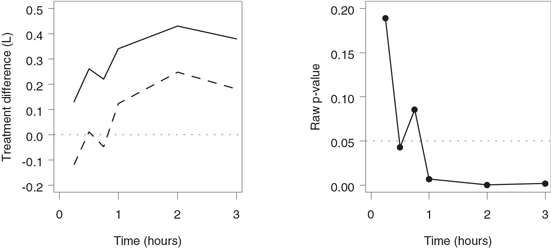
The output of Program 2.6 is shown in Figure 2.7. When reviewing the one-sided confidence limits and raw p-values in Figure 2.7, it is tempting to examine the results in a “step-up” manner—i.e., to start with the first spirometry measurement and stop testing as soon as a statistically significant mean difference is observed (30 minutes after the allergen challenge). However, this approach does not control the familywise error rate. To protect the Type I error rate, fixed-sequence testing should be performed in a sequentially rejective fashion. This means that each subsequent hypothesis is tested only if all previously tested hypotheses have been rejected. This can be achieved if we examine the treatment differences in a “step-down” fashion—i.e., by starting with the last spirometry measurement and working backwards. With the step-down approach, the lower 95% confidence limit includes zero (or, equivalently, a non-significant p-value is observed) for the first time 45 minutes after the allergen inhalation. This means that a statistically significant separation between the mean FEV1 values in the two groups occurs 1 hour after the allergen challenge.
Figure 2.7 Treatment comparisons in the allergen-induced asthma trial. Left-hand panel: Mean treatment difference (—) and lower confidence limit (- - -) by time. Right-hand panel: Raw p-values by time.
This example illustrates the importance of “monotonicity” assumptions in fixed-sequence testing. Fixed-sequence testing methods perform best when the magnitude of the treatment effect can be assumed to change monotonically with respect to time or dose. When the assumption is not met, fixed-sequence tests are prone to producing spurious results. Coming back to the data summarized in Table 2.5, suppose that the mean difference in FEV1 changes between the experimental drug and the placebo is very small at the last spirometry measurement. If the associated p-value is not significant, one cannot determine the onset of therapeutic effect despite the fact that the experimental drug separated from the placebo at several time points.
Similarly, Hsu and Berger (1999) proposed to use intersection-union testing methods to help" identify the minimum effective dose (MED) in dose-finding trials. One starts with comparing the highest dose to the placebo and then steps down to the next dose if the comparison is significant. Testing continues in this manner until an ineffective dose is reached. Hsu and Berger argued that the described algorithm guarantees a contiguous set of efficacious doses. This contiguous set of doses is helpful for establishing a therapeutic window for drug regimens. Note that the outlined testing procedure can be used only if the response increases monotonically with dose. It is clear that one runs a risk of missing the MED if the true dose-response curve is umbrella-shaped.
As a side note, one can also perform multiple inferences in studies with serial measurements per subject by taking into account the longitudinal correlation. See Littell et al. (1996) for a review of repeated-measures models for continuous endpoints and associated multiple testing procedures with a large number of SAS examples.
2.4.2 Hsu-Berger Method for Constructing Simultaneous Confidence Intervals
In the previous subsection, we described the use of fixed-sequence testing in applications with a priori ordered hypotheses and demonstrated how to interpret unadjusted confidence intervals and p-values in order to" identify the onset of therapeutic effect in an allergen-induced asthma trial. An interesting feature of fixed-sequence tests is that, unlike closed tests, they are easily inverted to set up simultaneous confidence intervals for the parameters of interest. In this subsection we will briefly outline a stepwise method proposed by Hsu and Berger (1999) for constructing simultaneous confidence sets.
Consider a clinical trial with two treatment groups (experimental drug and placebo) in which a continuous endpoint is measured at m consecutive time points. The numbers of patients in the two groups are denoted by n1 and n2. Let Yijk denote the measurement collected from the jth patient in the ith treatment group at the kth time point. Assume that Yijk is normally distributed with mean μik and variance σ2k
Hk={μ1k−μ2k≤δ}, k=1,…,m,
where δ denotes the clinically relevant difference. The hypotheses are logically ordered and thus they can be tested in a step-down manner using a fixed-sequence procedure. Let l equal the index of the first retained hypothesis if at least one hypothesis has been retained. If all hypotheses have been rejected, let l = 0.
Hsu and Berger (1999) proposed the following algorithm for setting up lower confidence limits for the true treatment difference at the kth time point, i.e., μ1k — μ2k, k = 1,…, m. First, construct one-sided confidence intervals for the treatment differences at each time point (as was done in Program 2.6). The confidence interval for μ1k — μ2k is given by
Ik={μ1k−μ2k≥ˆμ1k−ˆμ2k−tα,vsk},
where
ˆμik=ni∑j=1Yijk/ni,Sk=ˆαk√1/n1+1/n2
and ˆσk
ˆμ1k−ˆμ2k−tα,vsk≥δ, k=1,…,m,
set the lower limit of the adjusted confidence intervals to the same value, namely,
mink=1,...,m(ˆμ1k−ˆμ2k−tα,vsk).
Otherwise, the adjusted confidence interval Ĩk is defined as
˜Ik={μ1k−μ2k≥min(δ,ˆμ1k−ˆμ2k−tα,vsk)}
for k = l,…,m and Ĩk is empty for k = 1,…, l – 1.
We can see from the outlined algorithm that the adjusted confidence intervals for the treatment difference are constructed in a step-down manner. Beginning with the last time point, the one-sided confidence interval for μ1k — μ2k is given by
{μ1k−μ2k≥δ}
if the fixed-sequence test has rejected the null hypotheses Hk,…, Hm, and the unadjusted one-sided 100(1 — α)% confidence interval is used otherwise. Hsu and Berger (1999) proved that the coverage probability of the constructed set is no less than 100(1 — α)%.
To illustrate the Hsu-Berger method, consider the data collected in the allergen-induced asthma trial (see Table 2.5) and assume that δ is equal to zero; that is, the trial is declared successful if any statistically significant treatment is observed. Program 2.7 employs the Hsu-Berger procedure to construct the adjusted lower 95% confidence limits for the mean difference in FEV1 changes between the two treatment groups (experimental group minus placebo).
Program 2.7 Hsu-Berger simultaneous confidence intervals
proc sort data=summary;
by descending time;
data rejcount;
set summary nobs=m;
retain index 1 minlower 100;
if lower>0 and index=_n_ then index=_n_+1;
if lower<minlower then minlower=lower;
keep index minlower;
if _n_=m;
data adjci;
set summary nobs=m;
if _n_=1 then set rejcount;
if index=m+1 then adjlower=minlower;
if index<=m and _n_<=index then adjlower=min(lower,0);
axis1 minor=none label=(angle=90 "Treatment difference (L)")
order=(-0.2 to 0.5 by 0.1);
axis2 minor=none label=("Time (hours)") order=(0 to 3 by 1);
symbol1 value=none i=j color=black line=1;
symbol2 value=none i=j color=black line=20;
proc gplot data=adjci;
plot meandif*time lower*time/overlay frame vaxis=axis1 haxis=axis2
vref=0 lvref=34;
run;
axis1 minor=none label=(angle=90 "Treatment difference (L)")
order=(-0.2 to 0.5 by 0.1);
axis2 minor=none label=("Time (hours)") order=(0 to 3 by 1);
symbol1 value=none i=j color=black line=1;
symbol2 value=none i=j color=black line=20;
proc gplot data=adjci;
plot meandif*time adjlower*time/overlay frame vaxis=axis1 haxis=axis2
vref=0 lvref=34;
run;
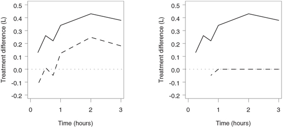
The output of Program 2.7 is shown in Figure 2.8. The left-hand panel of the figure displays the unadjusted lower 95% confidence limits for the treatment difference in FEV1 changes and is" identical to the left-hand panel of Figure 2.6. It is reproduced here to facilitate the comparison with the right-hand panel, which presents the simultaneous 95% confidence limits computed using the Hsu-Berger algorithm. The unadjusted confidence intervals exclude zero at 3 hours, 2 hours and 1 hour after the allergen challenge and thus, according to the Hsu-Berger algorithm, the adjusted lower limits are set to zero at these time points. The hypothesis of no treatment difference is retained for the first time 45 minutes after the allergen inhalation, which implies that the adjusted confidence interval is equal to the unadjusted one at 45 minutes and is undefined at the first two spirometry measurements.
2.4.3 Summary
Fixed-sequence tests introduced in this section provide an attractive alternative to closed tests when the null hypotheses of interest are naturally ordered. In the presence of an a priori ordering, one can test the individual hypotheses in a sequentially rejective fashion without any adjustment for multiplicity. Each subsequent hypothesis is tested only if all previously tested hypotheses have been rejected.
Figure 2.8 Hsu-Berger simultaneous confidence intervals in the allergen-induced asthma trial. Left-hand panel: Mean treatment difference (—) and unadjusted lower confidence limit (- - -) by time. Right-hand panel: Mean treatment difference (—) and Hsu-Berger adjusted lower confidence limit (- - -) by time.
In clinical trials, it is natural to carry out fixed-sequence tests when the endpoint is measured under several different conditions—for instance, when testing is performed over time and thus the order of null hypotheses is predetermined. As an example, it was demonstrated in this section how to perform fixed-sequence inferences to" identify the onset of therapeutic effect in an asthma study. Fixed-sequence testing methods are known to perform best when the magnitude of treatment effect can be assumed to change monotonically with respect to time or dose. When the assumption is not met, fixed-sequence tests are likely to produce spurious results.
Unlike closed testing procedures described in Section 2.3, fixed-sequence procedures are easily inverted to construct simultaneous confidence intervals for the parameters of interest. To illustrate this interesting feature of fixed-sequence tests, this section briefly outlined a stepwise method proposed by Hsu and Berger (1999) for constructing simultaneous confidence sets.
2.5 Resampling-Based Testing Methods
This section provides a brief overview of the method of resampling-based multiplicity adjustment introduced in Westfall and Young (1989) and further developed in Westfall and Young (1993) and Westfall et al. (1999).
Consider the problem of simultaneously testing m null hypotheses H1,…, Hm and let p1,…, pm denote the p-values generated by the associated significance tests. Assume for a moment that we know the exact distribution of the individual p-values. Westfall and Young (1989) proposed to define adjusted p-values ˜p1,…,˜pm
˜pi=P {min(P1,…,Pm)≤pi}, i=1,…,m,
where P1,…,Pm are random variables that follow the same distribution as p1,…, pm assuming that the m null hypotheses are simultaneously true. Once the adjusted p-values have been computed, the null hypotheses can be tested in a straightforward manner. Specifically, the null hypothesis Hi is rejected if ˜pi≤α
Westfall and Young (1993, Section 2.6) also derived adjusted p-values associated with a step-down procedure similar to that proposed by Holm (1979). The adjusted p-values are given by
˜p(1)=P {min(P1,…,Pm)≤p1},
˜p(i)=max[˜p(i−1)P {min(P(i),…,Pm)≤p(i)}], i=2,…,m.
Again, the computations are done under the assumption that H1,…, Hm are simultaneously true. This testing procedure will dominate the Holm, Hommel or any other step-down procedure in terms of power since it incorporates the stochastic dependence among the individual p-values into the decision rule.
Bootstrap Resampling
A natural question that comes up at this point is how to compute the adjusted p-values defined above when we do not know the exact distribution of the p-values observed in an experiment. Westfall and Young (1989, 1993) described a resampling-based solution to this problem. The unknown joint distribution of the p-values can be estimated using the bootstrap.
The bootstrap methods have found a variety of applications since they were introduced in the pioneering paper of Efron (1979). A large number of references on the bootstrap can be found in Efron and Tibshirani (1993). To briefly review the rationale behind the Efron bootstrap methodology, consider a sample
(X1,…, Xn) of independent," identically distributed observations from an unknown distribution. We are interested in computing multiplicity-adjusted p-values using the Westfall-Young formula. The bootstrap methodology relies on resampling with replacement. Let (X*1,…,X*n
Suppose we have generated all possible bootstrap samples and computed raw bootstrap p-values from each of them. For each pi, calculate the proportion of bootstrap samples in which min (p*1,…,p*m) is less than or equal to pi. This quantity is a bootstrap estimate of the true adjusted p-value (it is often called the ideal bootstrap estimate). The total number of all possible bootstrap samples generated from a given sample of observations is extremely large. It grows exponentially with increasing n and thus" ideal bootstrap estimates are rarely available. In all practical applications" ideal bootstrap estimates are approximated using Monte Carlo methods.
EXAMPLE: Ulcerative Colitis Trial
The Westfall-Young resampling-based multiplicity adjustment method is implemented in PROC MULTTEST (in fact, PROC MULTTEST was created to support this methodology). To show how to perform a resampling-based multiplicity adjustment in PROC MULTTEST, consider a data set from a dose-finding ulcerative colitis trial in which a placebo (Dose 0) is compared to three doses of an experimental drug (with 12 patients in each treatment group). The primary trial endpoint is the reduction in a 15-point endoscopy score in the four treatment groups. The endoscopy scores are not normally distributed; however, they are likely to follow a location shift model which is effectively handled by PROC MULTTEST.
Let y0j and yij, i = 1, 2, 3, denote the changes in the endoscopy score in the jth patient in the placebo and ith dose group, respectively. Since there are 12 patients in each treatment group, the within-group residuals εij are defined as
εij=yij−11212∑j=1yij, i=0,1,2,3, j=1,…,12.
Let p1, p2 and p3 be the raw p-values produced by the three two-sample t-tests comparing the individual doses of the experimental drug to the placebo.
The following is an algorithm for computing Monte Carlo approximations to the multiplicity-adjusted p-values in the ulcerative colitis trial example:
• Select a bootstrap sample ε*i j , i = 0, 1, 2, 3, j = 1,…, 12, by sampling with replacement from the pooled sample of 48 within-group residuals. The obtained residuals can be assigned to any treatment group because the sampling process is performed under the assumption that the three doses of the drug are no different from the placebo.
• Let p*1, p*2 and p*3 denote the p-values computed from each bootstrap sample using the two-sample t -tests for the three dose-placebo comparisons.
• Repeat this process a large number of times.
• Lastly, consider each one of the raw p-values (for example, p1) and compute the proportion of bootstrap samples in which min (p*1, p*2, p*3) was less than or equal to p1 . This is a Monte Carlo approximation to the true adjusted p1 . Monte Carlo approximations for the multiplicity-adjusted p2 and p3 are computed in a similar manner.
Program 2.8 estimates the adjusted p-values for the three dose-placebo comparisons using single-step and stepwise algorithms (BOOTSTRAP and STEPBOOT options) that are conceptually similar to single-step and stepwise marginal tests discussed earlier in Sections 2.2 and 2.3. The adjusted p-values are computed based on the two-sample t -test using 10,000 bootstrap samples.
Program 2.8 Resampling-based multiplicity adjustment in the dose-finding ulcerative colitis trial
data colitis;
do dose=″Dose 0″, ″Dose 1″, ″Dose 2″, ″Dose 3″;
do patient=1 to 12;
input reduct @@; output;
end;
end;
datalines;
| -2 | -1 | -1 | -1 | 0 | 0 | 0 | 0 | 0 | 2 | 4 | 5 |
| -1 | 0 | 1 | 1 | 1 | 2 | 3 | 3 | 3 | 4 | 7 | 9 |
| 1 | 2 | 2 | 3 | 3 | 3 | 3 | 3 | 4 | 6 | 8 | 8 |
| 1 | 4 | 5 | 5 | 6 | 7 | 7 | 7 | 8 | 8 | 11 | 12 |
;
proc multtest data=colitis bootstrap stepboot seed=47292 n=10000;
class dose;
test mean(reduct);
contrast ″Dose 0 vs Dose 1″ 1 -1 0 0;
contrast ″Dose 0 vs Dose 2″ 1 0 -1 0;
contrast ″Dose 0 vs Dose 3″ 1 0 0 -1;
run;
Output from Program 2.8
| p-Values | ||||
| Variable | Contrast | Raw | Bootstrap | Stepdown Bootstrap |
| reduct | Dose 0 vs Dose 1 | 0.0384 | 0.0973 | 0.0397 |
| reduct | Dose 0 vs Dose 2 | 0.0028 | 0.0090 | 0.0067 |
| reduct | Dose 0 vs Dose 3 | <.0001 | <.0001 | <.0001 |
Output 2.8 displays the raw and bootstrap-adjusted p-values for each of the three dose-placebo comparisons computed by PROC MULTTEST. The single-step resampling-based procedure has rejected two null hypotheses. The two highest doses of the experimental drug demonstrated a significantly larger mean reduction in the endoscopy score compared to the placebo. The stepwise procedure has produced a smaller adjusted p -value for the placebo versus lowest dose comparison and therefore rejected all three null hypotheses. As in the case of multiple tests based on marginal p-values, the stepwise resampling-based test is more powerful than the single-step resampling-based test. Note that, even though the bootstrap resampling is performed under the assumption that all three null hypotheses are true, the resulting testing procedure controls the familywise error rate in the strong sense.
The resampling-based methodology is sometimes criticized because it relies heavily on Monte Carlo approximations. Westfall and Young (1993) also introduced permutation versions of their bootstrap tests and showed that permutation testing methods often deliver exact solutions. Westfall and Young demonstrated via simulations that permutation multiple testing procedures are generally more conservative than bootstrap procedures. The difference between the two methods is rather small in the continuous case and becomes more pronounced in the binary case. Permutation-based multiplicity adjustments are available in PROC MULTTEST and can be requested using the PERMUTATION and STEPPERM options.
Subset Pivotality Condition
The concept of subset pivotality is one of the key concepts of resampling-based inference. It was introduced by Westfall and Young (1993) to describe conditions under which resampling-based multiple tests control the familywise error rate in the strong sense. To define the subset pivotality condition, consider again the null hypotheses H1 , … , Hm . Partition the hypotheses into two subsets. The subset pivotality condition holds if the joint distribution of the p-values corresponding to the hypotheses in the first subset does not depend on the hypotheses in the second subset for any partitioning scheme. In other words, the hypotheses in the second subset may be true or false but this will not affect our inferences with respect to the hypotheses in the first subset. See Westfall and Young (1993, Section 2.2) for details and examples.
The subset pivotality condition is met in a large number of practical situations. There are, however, some exceptions, the most important of which is the case of binary outcomes. The subset pivotality condition does not hold in problems involving multiple pairwise or treatment-control comparisons of proportions. In simple terms, this is caused by the heteroscedastic nature of binary data. Under normal theory, different populations can have a common variance even if their means are dramatically different. In contrast, the variances of sample proportions are constant across several populations only if the underlying true proportions are all the same. Westfall et al. (1999, Section 12.3) gave an example of a study with a binary endpoint in which a permutation multiple testing procedure based on the Fisher exact test produced a clearly incorrect result.
To alleviate this problem, Westfall and Young (1993) recommended to apply a variance-stabilizing transformation (e.g., the well-known arcsine transformation) before performing a resampling-based multiplicity adjustment. The Freeman-Tukey test in PROC MULTTEST is based on the arcsine transformation and generally does a better job in terms of controlling the overall Type I error rate than the Fisher exact test.
Program 2.9 compares the performance of the one-sided Fisher exact and Freeman-Tukey tests on a data set similar to the one used by Westfall et al. (1999, Program 12.5). The Fisher and Freeman-Tukey tests are requested in the program by using the FISHER and FT options in the TEST statement of PROC MULTTEST.
Program 2.9 Multiple testing procedures based on Fisher exact and Freeman-Tukey tests
data trouble;
input group outcome count @@;
datalines;
| 1 0 4 | 1 1 0 | 2 0 1 | 2 1 3 | 3 0 3 | 3 1 1 |
;
proc multtest data=trouble stepboot seed=443 n=20000;
title ″Adjustment based on the Fisher exact test″;
class group;
freq count;
test fisher(outcome/lower);
contrast ″1 vs 2″ 1 -1 0;
contrast ″1 vs 3″ 1 0 -1;
contrast ″2 vs 3″ 0 1 -1;
proc multtest data=trouble stepboot seed=443 n=20000;
title ″Adjustment based on the Freeman-Tukey test″;
class group;
freq count;
test ft(outcome/lower);
contrast ″1 vs 2″ 1 -1 0;
contrast ″1 vs 3″ 1 0 -1;
contrast ″2 vs 3″ 0 1 -1;
run;
Output from Program 2.9
Adjustment based on the Fisher exact test
| p-Values | |||
| Variable | Contrast | Raw | Bootstrap Stepdown |
| outcome | 1 vs 2 | 0.0714 | 0.0698 |
| outcome | 1 vs 3 | 0.5000 | 0.4956 |
| outcome | 2 vs 3 | 0.9857 | 0.7972 |
Adjustment based on the Freeman-Tukey test
| p-Values | |||
| Variable | Contrast | Raw | Bootstrap Stepdown |
| outcome | 1 vs 2 | 0.0109 | 0.0698 |
| outcome | 1 vs 3 | 0.1522 | 0.3361 |
| outcome | 2 vs 3 | 0.8975 | 0.9162 |
Output 2.9 shows that all three adjusted p-values produced by the Fisher exact test are less than the corresponding raw p-values. This is obviously a serious error. In repeated sampling, this procedure will demonstrate excessive Type I error rates. In contrast, the adjusted p-values associated with the Freeman-Tukey test are greater than the raw p-values. Generally, multiple testing procedures based on the Freeman-Tukey test have a more reasonable Type I error rate. See Westfall and Wolfinger (2000) for more details about subset pivotality and PROC MULTTEST documentation, and Westfall et al. (1999, Section 12.3) for other approaches to resampling-based multiple inference in binary applications.
2.5.1 Summary
This section briefly described the method of resampling-based multiplicity adjustment introduced by Westfall and Young (1989). The resampling-based methodology is very appealing in clinical applications because it combines the simplicity of marginal tests and the power of tests that make distributional assumptions. Resampling-based multiple tests are easy to implement and yet they can be applied to a wide variety of settings including univariate and multivariate models. PROC MULTTEST has extensive capabilities for carrying out bootstrap- and permutation-based multiple tests. For a further discussion of resampling-based multiplicity adjustments, their applications and PROC MULTTEST examples, see Westfall et al. (1999).
2.6 Testing Procedures for Multiple Endpoints
A large number of clinical trials employ multiple co-primary endpoints to study the efficacy or safety of new therapies. Multiple endpoints are popular in a clinical trial setting for several reasons. In their review of clinical trials with multiple outcome measures, Huque and Sankoh (1997) pointed out that it is often difficult to fully characterize the efficacy profile of an experimental therapy using a single endpoint when the disease of interest has a complex etiology. They illustrated their point using ulcerative colitis trials, which commonly include a variety of patient and physician assessments. Drug developers encounter similar problems in many other areas. For example, it is known that no single outcome variable defines a clinically relevant therapeutic benefit for patients with lupus (Siegel, 1999). This section describes several approaches to the simultaneous analysis of multiple endpoints in a clinical trial setting. We will discuss parametric and resampling-based testing procedures for multiple endpoints.
2.6.1 Global Tests for Multiple Endpoints
Consider a clinical trial in which g therapies are compared to each other and the therapeutic effect of each of them is assessed using m continuous endpoints. There are ni patients in the ith treatment group and n=∑gi=1ni. Let Xijk denote a normally distributed measurement taken from the jth patient in the ith treatment group with respect to the kth endpoint. Let μ ik and ơk denote the mean and standard deviation of Xijk , respectively. Further, assume a common correlation matrix in the g treatment groups and denote it by R . We are interested in constructing a test that combines the evidence from the individual endpoints, i.e., a test that evaluates the drug effect in a global fashion.
In a clinical trial setting, there is an important distinction between favorable and unfavorable treatment differences. A good global test needs to be able to detect the direction of treatment differences with respect to the individual endpoints. Assume that larger values of Xijk reflect a clinical improvement. In mathematical terms, we wish to test the global null hypothesis H of no treatment effect,
H={μ1k=μ2k=…=μgk, k=1,…,m},
against a “one-sided” alternative hypothesis H* that represents an improvement with respect to some or all of the m endpoints,
H*={μtk≤μuk with at least one strict inequalityfor some t and u, k=1,…,m}.
Note that directionless tests such as the Hotelling T2 test will not work in clinical applications because they test the global null hypothesis H against a “two-sided” alternative representing any departure from H . Clinical statisticians are interested in methods for directing Hotelling-type tests toward narrow, clinically important alternatives.
Tests Based on Marginal p-Values
As we stressed in Sections 2.2 and 2.3, multiple tests based on marginal p-values are widely used in the analysis of multiple endpoints. Single-step and stepwise marginal tests such as the Bonferroni or Holm tests are easy to implement in SAS using PROC MULTTEST. It is important to remember that marginal tests for multiple endpoints ignore the stochastic dependence among the individual endpoints. As a result, these tests are often very conservative in a clinical setting because multiple endpoints are typically biologically related and thus likely to exhibit a significant amount of correlation. Several authors presented the results of Monte Carlo simulations conducted to assess the performance of marginal tests such as the Bonferroni test and to compare it to the performance of tests that account for the correlation among the endpoints. Pocock, Geller and Tsiatis (1987) indicated that the Bonferroni test is most powerful when a significant improvement is observed only with respect to one of the endpoints, which is rarely the case in clinical applications. On the other hand, the Bonferroni test seriously lacks power in more realistic scenarios involving favorable changes in all of the endpoints.
EXAMPLE: Rheumatoid Arthritis Trial
We will illustrate the limitations of marginal tests for multiple endpoints using a small “proof-of-concept” trial in patients with rheumatoid arthritis. The efficacy of rheumatoid arthritis therapies is typically assessed using the American College of Rheumatology (ACR) definition of improvement (Felson et al., 1995). This definition was derived from seven measures of disease activity, including joint counts, patient and physician assessments, and an inflammation biomarker. The ACR response criterion is typically defined based on a 20% improvement in some or all of the listed measures. The use of this response criterion is required in registration trials for therapies aimed at improving the signs and symptoms of rheumatoid arthritis.
Note that the ACR response criterion is constructed by dichotomizing continuous outcome variables. It is well known that one should generally expect a loss of power in the statistical analysis when a continuous endpoint is converted into a categorical one. For this reason, the ACR response criterion is less frequently used as the primary endpoint in early proof-of-concept trials in patients with rheumatoid arthritis. Global tests based on some of the continuous endpoints comprising the ACR definition of improvement are generally more powerful than ACR response analyses in this setting.
Consider a clinical trial conducted to compare a new rheumatoid arthritis therapy to a placebo. Twenty-four rheumatoid arthritis patients were enrolled in the trial. The primary analysis in this trial was based on the number of swollen joints (SJC), number of tender joints (TJC), physician global assessment (PHA) and patient global assessment (PTA). The number of swollen and tender joints was computed using a 28-joint count, and the physician and patient global assessments were performed on a 100-mm visual analog scale. The changes from baseline in the four efficacy measures are summarized in Program 2.10.
Program 2.10 Rheumatoid arthritis data
data ra;
input group $ sjc tjc pta pha @@;
datalines;
| Placebo | -5 | -9 | -14 | -21 | Placebo | -3 | -7 | -5 | -25 |
| Placebo | -7 | -4 | -28 | -15 | Placebo | -3 | 0 | -17 | -6 |
| Placebo | -4 | -1 | -5 | 5 | Placebo | 0 | 5 | -8 | -11 |
| Placebo | -3 | 1 | 15 | 0 | Placebo | 2 | 6 | 15 | 27 |
| Placebo | -1 | -4 | -11 | -8 | Placebo | 0 | 1 | 8 | 12 |
| Placebo | 2 | -2 | 6 | -9 | Placebo | 8 | 2 | 11 | 33 |
| Therapy | -7 | -1 | -21 | -9 | Therapy | -6 | -11 | -36 | -12 |
| Therapy | -3 | -7 | -14 | -21 | Therapy | -4 | 2 | 10 | -10 |
| Therapy | -11 | -4 | -28 | -45 | Therapy | -4 | -1 | -11 | -23 |
| Therapy | -3 | -1 | -7 | -15 | Therapy | -5 | -9 | -36 | -15 |
| Therapy | -4 | -9 | -35 | -32 | Therapy | -11 | -10 | -47 | -31 |
| Therapy | 3 | -1 | 6 | 17 | Therapy | -1 | -9 | -5 | -27 |
| ; |
The four selected outcome measures represent closely related aspects of patient outcome and it should not be surprising that they are highly correlated. The sample correlation matrix is equal to
ˆR=[10.510.750.760.5110.720.650.750.7210.670.760.650.671].
Program 2.11 performs simple univariate analyses of the four efficacy endpoints using the two-sample t -tests under the assumption of equal variances (we used ods listing close to suppress the regular PROC TTEST output and ods listing to enable printing in PROC PRINT).
Program 2.11 Analysis of the rheumatoid arthritis data using univariate two-sample t-tests
ods listing close;
proc ttest data=ra;
class group;
var sjc tjc pta pha;
ods output ttests=ttest(where=(method=″Pooled″));
proc print data=ttest noobs label;
ods listing;
run;
Output from Program 2.11
| Variable | Method | Variances | t Value | DF | Pr >|t| |
| sjc | Pooled | Equal | 2.18 | 22 | 0.0403 |
| tjc | Pooled | Equal | 2.21 | 22 | 0.0375 |
| pta | Pooled | Equal | 2.43 | 22 | 0.0239 |
| pha | Pooled | Equal | 2.50 | 22 | 0.0205 |
Note that all four raw p-values in Output 2.11 are significant at the usual 5% level. However, if we employ a crude Bonferroni correction for multiplicity, our conclusions about the overall effect of the experimental therapy will change. The Bonferroni global test produces a non-significant p -value of 0.082 (this p -value equals 4 times the smallest raw p -value in Output 2.11).
Likelihood-Based Tests
Under normal theory, a natural choice for a hypothesis-testing problem with multiple endpoints is a likelihood ratio test. As pointed out in Wassmer, Reitmeir, Kieser and Lehmacher (1999), several authors (including Perlman (1969)) considered likelihood ratio tests for the one-sided problem outlined above. However, the likelihood-based solutions turned out to be very complex, especially in the case when the correlation matrix R is unknown. Since the likelihood ratio test for the multiple endpoint problem is computationally intractable, alternative solutions based on approximations were proposed in the literature. For instance, Tang, Gnecco and Geller (1989a) derived an approximation to the likelihood ratio test by suitably transforming the original data. Although the proposed approximate likelihood ratio test is more attractive than the full-blown likelihood ratio test, it still presents considerable computational problems. The null distribution of the test statistic developed by Tang, Gnecco and Geller belongs to the class of chi-bar-squared distributions and numerical integration is required to compute the associated critical points and p-values.
Ordinary Least Squares Test
A different and more flexible approach was proposed by O’Brien (1984). O’Brien developed a general method for testing for the global null hypothesis of no treatment effect based on a weighted sum of the individual test statistics. Suppose that the effect sizes associated with the individual endpoints are equal within each treatment group, i.e.,
μi1σ1=μi2σ2=…=μimσm, i=1,…,g.
Let λi denote the common effect size in the ith treatment group.
When the assumption of equal effect sizes is met, the complex multivariate problem of analyzing the m endpoints reduces to a simpler univariate problem of comparing the common effect sizes across the treatment groups. O’Brien (1984) proposed to estimate λ1, … ,λg using the method of ordinary least squares (OLS) and then perform across-group comparisons with the help of standard ANOVA techniques.
First, individual observations need to be standardized to ensure that the m endpoints are expressed in common units. Let
Yijk=(Xijk−mk)/sk,
where mk is the overall mean and sk is the usual pooled sample standard deviation for the kth endpoint. To carry out the O’Brien OLS test, combine the standardized observations across the m endpoints by defining
Y*ij=m∑k=1Yijk
and perform a one-way analysis of variance on these composite scores. The resulting F -test statistic follows the F distribution with g – 1 and n — mg degrees of freedom (it is worth noting that the F -test in a one-way ANOVA setting has more degrees of freedom in the denominator).
In two-arm studies, the two-sample t -test can be employed. It is interesting to note that the OLS t -test statistics can be expressed as
tOLS=1√J′ˆRJm∑k=1tk,
where tk is the usual t-test statistic for the kth endpoint, i.e.,
tk=ˆX1.k−ˆX2.kSk√1/n1+1/n2,
ˆR is the sample correlation matrix of the original observations, and J =[1 1 … 1]. (In other words, J′ˆRJ is the sum of all entries in the sample correlation matrix.) This representation of tOLS highlights the fact that the O’Brien OLS method simply combines the individual t -test statistics for each of the m endpoints with equal weights.
Let us now analyze the rheumatoid arthritis data introduced earlier in this section using the O’Brien OLS test. Figure 2.9 presents a simple plot of the data that indicates that the effect sizes associated with
Figure 2.9 Plot of the effect sizes associated with the physician global assessment (PHA), patient global assessment (PTA), number of swollen joints (SJC) and number of tender joints (TJC) in the placebo (△) and experimental (◯) groups in the rheumatoid arthritis trial the four efficacy measures are fairly consistent within the experimental and placebo groups. It is safe to conclude that the assumption of equal effect sizes is met.
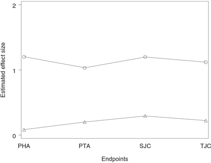
Program 2.12 assesses the overall effect of the experimental therapy on the selected efficacy measures of disease activity using the O’Brien OLS test. The program is based on the %GlobTest macro given in the Appendix. This powerful macro implements the O’Brien OLS test as well as three other global tests that will be introduced later in this section.
Program 2.12 Analysis of the rheumatoid arthritis data using the O’Brien OLS test
%GlobTest(dataset=ra,group=group,ngroups=2,varlist=sjc tjc pta pha,
test=″OLS″);
The %GlobTest macro has five arguments described below:
• DATASET is the data set to be analyzed.
• GROUP is the name of the group variable in the data set.
• NGROUPS is the number of groups in the data set.
• VARLIST is the list of variable names corresponding to the multiple endpoints of interest.
• TEST is the name of the test to be used, OLS test (“OLS”), GLS test (“GLS”), modified GLS test (“MGLS”) or rank-sum test (“RS”), respectively.
Output from Program 2.12
| F-value | ndf | ddf | Global p-value |
| 7.73 | 1 | 16 | 0.0134 |
Output 2.12 shows that the p -value associated with the O’Brien OLS test equals 0.0134. Comparing this finding with the Bonferroni-adjusted p -value of 0.082 displayed in Output 2.11, we see that incorporating the correlation structure into the decision rule has resulted in a substantial increase in power. Moreover, due to strong positive dependence among the four variables, the O’Brien OLS p -value is more significant than any of the raw p-values from the univariate t -tests. Based on the OLS test, we conclude that the experimental therapy is statistically superior to the placebo when the four efficacy measures are treated as one instrument.
We have considered a multiple endpoint scenario in which the effect sizes were fairly similar within the treatment groups. The O’Brien OLS test also performs well when the effect sizes associated with the multiple endpoints vary within treatment groups. However, it loses power as the spread in the effect sizes increases. One needs to carefully examine both the univariate p-values and the global OLS p -value when no treatment effect is observed with respect to some of the endpoints, because the OLS test may break down in this situation.
Generalized Least Squares Test
Along with the OLS test, O’Brien (1984) proposed a global test based on a generalized least squares (GLS) estimate of the treatment effect under the assumption of equal effect sizes. The GLS test is more efficient than the OLS test in the presence of heteroscedasticity because it better accounts for the underlying correlation structure.
The important difference between the OLS and GLS approaches is that the GLS test statistic is based on a weighted sum of individual test statistics with the weights reflecting the correlation among multiple endpoints. To define the test statistic, consider again normally distributed observations Xijk . As with the OLS test, we first standardize the individual observations and let
Yijk=(Xijk−mk)/sk.
Now, to combine the standardized observations across the m endpoints, we will take into account the correlation structure. Let rtu denote the ( t , u ) entry in the inverse of the sample correlation matrix ˆR,
ˆR−1=[r11⋯r1m⋮⋱⋮rm1⋯rmm].
The composite scores Y*ij are defined as
Y*ij=m∑t=1m∑u=1rtuYiju
and thus endpoints receive greater weights when they are less correlated with the other endpoints. The computed composite scores are analyzed using a one-way analysis of variance. The GLS F -test statistic follows the F distribution with g – 1 and n — mg degrees of freedom.
Although the GLS test is generally more powerful than the OLS test, it may be less attractive in clinical applications because it is prone to producing uninterpretable results. As shown above, the weighting scheme in the GLS test is based on the inverse of the sample correlation matrix and it is theoretically possible that some of the endpoints can receive negative weights. Clinically, this means that the GLS test can reject the global null hypothesis of no treatment effect even if the new therapy is inferior to the control on all of the endpoints. See Pocock, Geller and Tsiatis (1987) and Follmann (1995) for a detailed discussion of this phenomenon and examples.
To fix the outlined problem, Tang, Geller and Pocock (1993) proposed to modify the O’Brien GLS test in such a way that individual endpoints always receive non-negative weights. The modified GLS test is based on the composite scores given by
Y*ij=m∑t=1√rttYijt.
As explained in Tang, Geller and Pocock (1993), this choice of weights often possesses an important maximin property. The modified GLS test maximizes the minimum power over all treatment differences in the favorable direction.
Program 2.13 analyzes the rheumatoid arthritis data using both the GLS test and its modification proposed by Tang, Geller and Pocock (1993). The program utilizes the %GlobTest macro.
Program 2.13 Analysis of the rheumatoid arthritis data using the O’Brien GLS test and modified GLS test proposed by Tang, Geller and Pocock (1993)
%GlobTest(dataset=ra,group=group,ngroups=2,varlist=sjc tjc pta pha,
test=″GLS″);
%GlobTest(dataset=ra,group=group,ngroups=2,varlist=sjc tjc pta pha,
test=″MGLS″);
Output from Program 2.13
| O’Brien GLS test | |||
| F-value | ndf | ddf | Global p-value |
| 7.41 | 1 | 16 | 0.0151 |
| Modified O’Brien GLS test | |||
| F-value | ndf | ddf | Global p-value |
| 7.71 | 1 | 16 | 0.0135 |
Output 2.13 lists the p-values produced by the regular and modified GLS tests. The modified GLS p-value equals 0.0135 and is virtually identical to that produced by the OLS test (see Output 2.12). The p-value associated with the GLS test is slightly less significant.
It is important to check whether the GLS test assigned non-negative weights to the four individual endpoints. The inverse of the sample correlation matrix ˆR is given by
ˆR−1=[3.450.87−1.95−1.880.872.56−1.7−1.19−1.95−1.73.560.18−1.88−1.190.183.08]
and it is easy to verify that the column sums in this matrix are positive. This implies that all four endpoints received positive weights and the GLS test is a valid test for comparing the experimental drug to the placebo with respect to the four selected endpoints.
The introduced O’Brien OLS and GLS methods can be extended to a variety of multiple endpoint problems involving normally distributed test statistics. For example, the next subsection introduces a nonparametric version of the O’Brien methods. Further, Pocock, Geller and Tsiatis (1987) demonstrated how the O’Brien GLS test can be applied to the analysis of binary and survival data. Other interesting extensions of this methodology are found in Follmann (1996) and Läauter (1996).
Rank-Sum Test
When clinical measurements are not normally distributed, one can perform an analysis of multiple endpoints using a nonparametric test proposed by O’Brien (1984). This rank-sum test is similar to the OLS and GLS testing procedures introduced earlier in the sense that it reduces the dimensionality of the multiple endpoint problem by combining data across the endpoints in a straightforward manner.
Consider the kth endpoint, and let Rijk denote the rank of Xijk in the pooled sample of g treatment groups with respect to the kth endpoint. The composite score Y*ij is defined for the jth patient in the ith treatment group as the sum of the obtained ranks, i.e.,
Y*ij=m∑t=1Rijt.
O’Brien proposed to analyze the composite scores by a one-way analysis of variance. The constructed test is conceptually similar to the Kruskal-Wallis test for a nonparametric comparison of multiple samples.
Program 2.14 carries out the O’Brien rank-sum test to compare the experimental drug to the placebo in the rheumatoid arthritis trial example. The rank-sum test statistic is computed by calling the %GlobTest macro.
Output 2.14 shows that the nonparametric p-value equals 0.0087 and is highly significant, which indicates that the experimental drug is clearly superior to the placebo when the four selected endpoints are examined simultaneously.
Program 2.14 Analysis of the rheumatoid arthritis data using the O’Brien rank-sum test
%GlobTest(dataset=ra,group=group,ngroups=2,varlist=sjc tjc pta pha,
test=″RS″);
Output from Program 2.14
| F-value | ndf | ddf | Global p-value |
| 8.28 | 1 | 22 | 0.0087 |
Resampling-Based Tests
Section 2.5 outlined applications of the Westfall-Young resampling-based methodology to multiplicity problems arising in the context of multiple comparisons. It is easy to extend this powerful methodology to the analysis of multiple endpoints. Westfall et al. (1999, Section 11.3) discussed the use of bootstrap and permutation tests in clinical trials with multiple outcome measures and showed how to carry out these tests using PROC MULTTEST.
Following Westfall et al. (1999), we will utilize resampling-based multiplicity adjustment techniques in the analysis of the rheumatoid arthritis data. As we have shown earlier in this section, a univariate approach to the analysis of the four outcome measures in the rheumatoid arthritis trial lacks power because it ignores the multivariate nature of the problem. To simultaneously test the four null hypotheses associated with the outcome measures of interest, we need to account for the stochastic dependence among the individual t -test statistics. The resampling-based methodology provides a way to estimate the underlying correlation structure and to compute adjusted p-values for each of the endpoints.
Program 2.15 computes adjusted p-values for the four endpoints in the rheumatoid arthritis trial example using the stepwise bootstrap algorithm.
Program 2.15 Analysis of the rheumatoid arthritis data using the resampling-based test
proc multtest data=ra stepboot n=10000 seed=57283;
class group;
test mean(sjc tjc pta pha);
contrast ″Treatment effect″ 1 -1;
run;
Output from Program 2.15
| p-Values | |||
| Variable | Contrast | Raw | Stepdown Bootstrap |
| sjc | Treatment effect | 0.0403 | 0.0702 |
| tjc | Treatment effect | 0.0375 | 0.0702 |
| pta | Treatment effect | 0.0239 | 0.0646 |
| pha | Treatment effect | 0.0205 | 0.0646 |
Output 2.15 demonstrates that the bootstrap-based multiplicity adjustment is not very efficient in this example. The global p-value associated with the bootstrap algorithm equals 0.0646 and is much larger than the O’Brien p-values in Output 2.12 and Output 2.13. It is important to point out that the disproportionately large adjusted p-values produced by the resampling-based procedure in this example do not imply that resampling-based inferences always lack power in statistical problems involving multiple endpoints. The observed difference between the resampling-based and O’Brien tests may simply reflect the fact that the latter testing procedures are very powerful under the assumption of equal effect sizes.
2.6.2 Individual Tests for Multiple Endpoints
The goal of global tests is to examine a significant overall difference across treatment groups with respect to the endpoints of interest. Global tests provide no information about the significance of treatment differences for individual endpoints. However, if the overall analysis yields a significant result, both the trial sponsor and regulatory reviewers are naturally interested in determining which of the individual treatment differences are significant after a proper adjustment for multiplicity.
Statistical inferences about individual endpoints are also very important in clinical trials designed to pursue multiple regulatory claims. It may not be appropriate to combine endpoints if they describe unrelated aspects of the patient response, in which case a global test of the endpoints needs to be replaced with suitably adjusted individual tests.
The easiest way to" identify individual significant outcome variables is to analyze the data using a multiple rather than a global test. For example, Troendle and Legler (1998) discussed the application of marginal tests in a multiple endpoint setting. All of the marginal tests described earlier in Sections 2.2 and 2.3 allow the clinical statistician to test the null hypotheses associated with each of the endpoints. Resampling-based tests for multiple endpoints also support inferences for individual outcome measures.
Alternatively, one can start with a global test (e.g., O’Brien and related tests) and utilize the closed testing principle introduced in Section 2.3 to step down to the individual hypotheses; see Lehmacher, Wassmer and Reitmeir (1991) and Westfall and Tobias (2000, Chapter 8) for more details. As we pointed out in Section 2.3, the closed testing principle provides clinical statisticians with a powerful tool for extending global tests to the level of individual hypotheses.
As an illustration, we will apply the method based on the closed testing principle to analyze the data from the rheumatoid arthritis trial example. The primary analysis in this trial was based on four efficacy measures, the swollen joint count, tender joint count, physician global assessment and patient global assessment. Let H1 , H2 , H3 , and H4 denote the null hypotheses of no treatment effect for the four endpoints. Consider a closed family of hypotheses associated with the four null hypotheses. The closed family contains 15 hypotheses representing all possible intersections of H1 , H2 , H3 and H4 (see Section 2.3 for a more detailed description of closed families of hypotheses). Each member of the closed family can be viewed as a global hypothesis and, therefore, can be tested using a global test, e.g., the O’Brien OLS test. To test the individual null hypotheses, we will need to combine the results and compute the adjusted p-values associated with H1 , H2 , H3 and H4 . The adjusted p-value for each individual null hypothesis is defined as the largest p-value for the intersection hypotheses that imply it.
In practice, adjusted p-values for H1 , H2 , H3 and H4 can be computed using the decision matrix algorithm introduced in Section 2.3.2. Program 2.16 utilizes the decision matrix approach to compute the adjusted p-values for the four efficacy variables in the rheumatoid arthritis trial. The %GlobTest macro is invoked in Program 2.16 to carry out the O’Brien OLS test for each member of the closed family of hypotheses associated with H1 , H2 , H3 and H4 .
Program 2.16 Analysis of the rheumatoid arthritis data using the closed version of the O’Brien OLS test
%let varname=sjc tjc pta pha;
data hyp;
length varlist $50;
array h{*} h1-h4;
do i=15 to 1 by -1;
string=put(i,binary4.);
hypnum=16-i;
do j=1 to 4;
h{j}=substr(string,j,1);
end;
varlist=″ ″;
do j=1 to 4;
if h{j}=1 then varlist=
trim(varlist) ||″ ″ || scan(″&varname″,j);
end;
output;
end;
keep hypnum h1-h4 varlist;
data pvalcomb;
%macro pval;
%do j=1 %to 15;
data _null_;
set hyp;
if hypnum=&j then call symput(″varlist″,trim(varlist));
run;
%GlobTest(ra,group,2,&varlist,″OLS″);
data pvalcomb;
set pvalcomb pval;
keep adjp;
run;
%end;
%mend pval;
%pval;
data decrule;
merge hyp pvalcomb(where=(adjp^=.));
array h{*} h1-h4;
array hyp{*} hyp1-hyp4;
do i=1 to 4;
hyp{i}=adjp*h{i};
end;
keep hyp1-hyp4;
proc means data=decrule noprint;
var hyp1-hyp4;
output out=indadjp(keep=adjp1-adjp4)
max(hyp1-hyp4)=adjp1-adjp4;
data indadjp;
set indadjp;
format adjp1-adjp4 6.4;
proc print data=indadjp noobs;
title ″Adjusted p-values for individual hypotheses″;
run;
Output from Program 2.16
| Adjusted p-values for individual hypotheses | |||
| adjp1 | adjp2 | adjp3 | adjp4 |
| 0.0403 | 0.0375 | 0.0239 | 0.0205 |
Output 2.16 lists the adjusted p-values for the individual null hypotheses in the rheumatoid trial example. The p-values correspond to the swollen joint count, tender joint count, physician global assessment and patient global assessment, respectively. It is instructive to compare these adjusted p-values to the raw p-values displayed in Output 2.11. Output 2.16 indicates that here we are dealing with a unique situation in which the adjusted p-values generated by the O’Brien OLS test are equal to the raw p-values produced by the univariate t -tests. Due to a common treatment effect across the variables considered, not only has the global OLS test yielded a significant result, but also the treatment differences with respect to all four endpoints are significant.
Needless to say, scenarios in which adjusted p-values are equal to raw p-values are very uncommon in clinical applications. Adjusted p-values for the individual endpoints are typically larger than the corresponding raw univariate p-values. In fact, one is likely to see non-significant adjusted p-values in univariate analyses following a significant global test. This happens because global tests are generally substantially more powerful than univariate inferences with respect to each individual endpoint. Theoretically, one may run into situations when the global test yields a significant result yet none of the adjusted univariate analyses is even remotely significant.
2.6.3 Summary
In this section we discussed statistical methods for the analysis of clinical trials with multiple endpoints and described the following testing procedures used in a clinical trial setting:
• Tests based on marginal p-values (e.g., the Bonferroni test) are often very conservative in clinical applications because they ignore the correlation among multiple endpoints.
• The ordinary least squares (OLS) test is an example of a global test for a simultaneous analysis of multiple endpoints. The OLS method combines equally weighted test statistics for the individual endpoints. The OLS test is most powerful under the assumption of equal effect sizes.
• The generalized least squares (GLS) test is a global test based on a weighted sum of individual test statistics. The test statistics are weighted to account for heteroscedasticity. The GLS test is generally more efficient than the OLS test but can sometimes produce uninterpretable results when it assigns negative weights to some of the endpoints.
• The modified generalized least squares test is similar to the GLS test. This test is set up in such a way that individual endpoints always receive non-negative weights.
• The rank-sum test is a natural extension of the OLS test to a nonparametric setting.
• Resampling-based testing procedures account for the stochastic dependence among multiple endpoints via bootstrap or permutation methods. These procedures can be used both for testing the global hypothesis and for testing the effects of individual endpoints.
The listed testing procedures for the analysis of clinical trials with multiple endpoints are easy to implement in SAS using PROC MULTTEST or the %GlobTest macro introduced in this section.
The section also addressed the issue of making inferences with respect to the individual endpoints after a global test has been carried out. Univariate analyses of this type are based on the closed testing principle and can be performed using the decision matrix algorithm.