

Chapter Four
USING THE DERIVATIVE
Contents
What Derivatives Tell Us About a Function and Its Graph
Detecting a Local Maximum or Minimum
Testing For Local Maxima and Minima
Concavity and Inflection Points
How Do You Locate an Inflection Point?
A Graphical Example: Minimizing Gas Consumption
Revenue and Elasticity of Demand
Elasticity of Demand for Different Products
The Carrying Capacity and the Point of Diminishing Returns
4.8 The Surge Function and Drug Concentration
4.1 LOCAL MAXIMA AND MINIMA
What Derivatives Tell Us About a Function and Its Graph
As we saw in Chapter 2, values of a function and its derivatives are related as follows:
- If f′ > 0 on an interval, then f is increasing on that interval.
- If f′ < 0 on an interval, then f is decreasing on that interval.
- If f″ > 0 on an interval, then the graph of f is concave up on that interval.
- If f″ < 0 on an interval, then the graph of f is concave down on that interval.
We now use these principles in conjunction with the derivative formulas from Chapter 3. For example, when we graph a function on a computer or calculator, we often see only part of the picture. The first and second derivatives can help identify regions with interesting behavior.
| Example 1 | Use a computer or calculator to sketch a useful graph of the function
|
| Solution | Since f is a cubic polynomial, we expect a graph that is roughly S-shaped. Graphing this function with −10 ≤ x ≤ 10, −10 ≤ y ≤ 10 gives the two nearly vertical lines in Figure 4.1. We know that there is more going on than this, but how do we know where to look?
Figure 4.1: Unhelpful graph of f (x) = x3 − 9x2 − 48x + 52 We use the derivative to determine where the function is increasing and where it is decreasing. The derivative of f is
To find where f′ > 0 or f′ < 0, we first find where f′ = 0; that is, where 3x2 − 18x − 48 = 0. Factoring gives
so x = −2 or x = 8. Since f′ = 0 only at x = −2 and x = 8, and since f′ is continuous, f′ cannot change sign on any of the three intervals x < −2, or −2 < x < 8, or 8 < x. How can we tell the sign of f′ on each of these intervals? The easiest way is to pick a point and substitute into f′. For example, since f′(−3) = 33 > 0, we know f′ is positive for x < −2, so f is increasing for x < −2. Similarly, since f′(0) = −48 and f′(10) = 72, we know that f decreases between x = −2 and x = 8 and increases for x > 8. Summarizing:
We find that f(−2) = 104 and f(8) = −396. Hence, on the interval −2 < x < 8 the function decreases from a high of 104 to a low of −396. (Now we see why not much showed up in our first calculator graph.) One more point on the graph is easy to get: the y-intercept, f(0) = 52. With just these three points we can get a much more helpful graph. By setting the plotting window to −10 ≤ x ≤ 20 and −400 ≤ y ≤ 400, we get Figure 4.2, which gives much more insight into the behavior of f(x) than the graph in Figure 4.1. In Figure 4.2, we see that part of the graph is concave up and part is concave down. We can use the second derivative to analyze concavity. We have
Thus, f″(x) < 0 when x < 3 and f″(x) > 0 when x > 3, so the graph of f is concave down for x < 3 and concave up for x > 3. At x = 3, we have f″(x) = 0. See Figure 4.2. Summarizing:
Figure 4.2: Useful graph of f(x) = x3 − 9x2 − 48x + 52. Notice that the scales on the x-and y-axes are different. |


Local Maxima and Minima
We are often interested in points such as those marked local maximum and local minimum in Figure 4.2. We have the following definition:
Suppose p is a point in the domain of f:
- f has a local minimum at p if f(p) is less than or equal to the values of f for points near p.
- f has a local maximum at p if f(p) is greater than or equal to the values of f for points near p.
We use the adjective “local” because we are describing only what happens near p. Local maxima and minima are sometimes called local extrema.
How Do We Detect a Local Maximum or Minimum?
In the preceding example, the points x = −2 and x = 8, where f′(x) = 0, played a key role in leading us to local maxima and minima. We give a name to such points:
For any function f, a point p in the domain of f where f′(p) = 0 or f′(p) is undefined is called a critical point of the function. In addition, the point (p, f (p)) on the graph of f is also called a critical point. A critical value of f is the value, f(p), at a critical point, p.
Notice that “critical point of f” can refer either to points in the domain of f or to points on the graph of f. You will know which meaning is intended from the context. A function may have any number of critical points or none at all. (See Figures 4.3–4.5.)

Figure 4.3: A quadratic: One critical point

Figure 4.4: f(x) = x3 + x + 1: No critical points
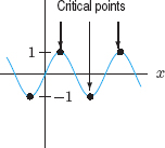
Figure 4.5: g(x) = sin x: Many critical points
Geometrically, at a critical point where f′(p) = 0, the line tangent to the graph of f at p is horizontal. At a critical point where f′(p) is undefined, there is no horizontal tangent to the graph—there is either a vertical tangent or no tangent at all. (For example, x = 0 is a critical point for the absolute value function f(x) = |x|.) However, most of the functions we will work with will be differentiable everywhere, and therefore most of our critical points will be of the f′(p) = 0 variety.
The critical points divide the domain of f into intervals on which the sign of the derivative remains the same, either positive or negative. Therefore, if f is defined on the interval between two successive critical points, its graph cannot change direction on that interval; it is either going up or going down. We have the following result:
If a function, continuous on the real line, has a local maximum or minimum at p, then p is a critical point of the function.
If a continuous function f has domain the interval a ≤ x ≤ b, then f may have local maxima or minima at the endpoints x = a and x = b, even if these points are not critical points of f.
Testing For Local Maxima and Minima
If f′ has different signs on either side of a critical point p with f′(p) = 0, then the graph changes direction at p and looks like one of those in Figure 4.6. We have the following criteria:
The First-Derivative Test for Local Maxima and Minima
Suppose p is a critical point of a continuous function f. Moving from left to right:
- If f′ changes from negative to positive at p, then f has a local minimum at p.
- If f′ changes from positive to negative at p, then f has a local maximum at p.

Figure 4.6: Changes in direction at a critical point, p: Local maxima and minima
Knowing the concavity of a function can also be useful in testing if a critical point is a local maximum or a local minimum. Suppose p is a critical point of f, with f′(p) = 0, so that the graph of f has a horizontal tangent line at p. If the graph is concave up at p, then f has a local minimum at p. Likewise, if the graph is concave down, f has a local maximum. (See Figure 4.7.) This suggests:

Figure 4.7: Local maxima and minima and concavity
The Second-Derivative Test for Local Maxima and Minima
Suppose p is a critical point of a continuous function f, and f′(p) = 0.
- If f″(p) > 0, then f has a local minimum at p.
- If f″(p) < 0, then f has a local maximum at p.
- If f″(p) = 0, then the test tells us nothing.
| Example 2 | Use the second-derivative test to confirm that f(x) = x3 − 9x2 − 48x + 52 has a local maximum at x = −2 and a local minimum at x = 8. |
| Solution | In Example 1, we calculated f′(x) = 3x2 − 18x − 48 = 3(x − 8)(x + 2), so f′(8) = f′(−2) = 0. Differentiating again gives f″(x) = 6x − 18. Since
the second-derivative test confirms that x = 8 is a local minimum and x = −2 is a local maximum. |
| Example 3 | (a) Graph a function f with the following properties:
|
| (b) Identify the critical points as local maxima, local minima, or neither. | |
| Solution | (a) We know that f(x) is increasing when f′(x) is positive, and f(x) is decreasing when f′(x) is negative. The function is increasing to the left of 2 and increasing to the right of 5, and it is decreasing between 2 and 5. A possible sketch is given in Figure 4.8. |
| (b) We see that the function has a local maximum at x = 2 and a local minimum at x = 5. |

Figure 4.8: A function with critical points at x = 2 and x = 5
Warning!
Not every critical point of a function is a local maximum or minimum. For instance, consider f(x) = x3, graphed in Figure 4.9. The derivative is f′(x) = 3x2 so x = 0 is a critical point. But f′(x) = 3x2 is positive on both sides of x = 0, so f increases on both sides of x = 0. There is neither a local maximum nor a local minimum for f(x) at x = 0.

Figure 4.9: A critical point that is neither a local maximum nor minimum.
| Example 4 | The value of an investment at time t is given by S(t). The rate of change, S′(t), of the value of the investment is shown in Figure 4.10. |
| (a) What are the critical points of the function S(t)? | |
| (b) Identify each critical point as a local maximum, a local minimum, or neither. | |
| (c) Explain the financial significance of each of the critical points. |
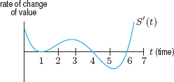
Figure 4.10: Graph of S′(t), the rate of change of the value of the investment
| Solution | (a) The critical points of S occur at times t when S′(t) = 0. We see in Figure 4.10 that S′(t) = 0 at t = 1, 4, and 6, so the critical points occur at t = 1, 4, and 6. |
| (b) In Figure 4.10, we see that S′(t) is positive to the left of 1 and between 1 and 4, that S′(t) is negative between 4 and 6, and that S′(t) is positive to the right of 6. Therefore S(t) is increasing to the left of 1 and between 1 and 4 (with a slope of zero at 1), decreasing between 4 and 6, and increasing again to the right of 6. A possible sketch of S(t) is given in Figure 4.11. We see that S has neither a local maximum nor a local minimum at the critical point t = 1, but that it has a local maximum at t = 4 and a local minimum at t = 6.
Figure 4.11: Possible graph of the function representing the value of the investment at time t |
|
| (c) At time t = 1 the investment momentarily stopped increasing in value, though it started increasing again immediately afterward. At t = 4, the value peaked and began to decline. At t = 6, it started increasing again. |

| Example 5 | Find the critical point of the function f(x) = x2 + bx + c. What is its graphical significance? |
| Solution | Since f′(x) = 2x + b, the critical point x satisfies the equation 2x + b = 0. Thus, the critical point is at x = −b/2. The graph of f is a parabola and the critical point is its vertex. See Figure 4.12. |

Figure 4.12: Critical point of the parabola f(x) = x2 + bx + c. (Sketched with b, c > 0)
Problems for Section 4.1
In Problems 1–4, indicate all critical points of the function f. How many critical points are there? Identify each critical point as a local maximum, a local minimum, or neither.
1.
2.
3.

4.

5. (a) Graph a function with two local minima and one local maximum.
(b) Graph a function with two critical points. One of these critical points should be a local minimum, and the other should be neither a local maximum nor a local minimum.
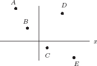
6. Graph two continuous functions f and g, each of which has exactly five critical points, the points A–E in Figure 4.13, and that satisfy the following conditions:
(a) f(x) → ∞ as x → −∞ and f(x) → ∞ as x → ∞
(b) g(x) → −∞ as x → −∞ and g(x) → 0 as x → ∞
7. During an illness a person ran a fever. His temperature rose steadily for eighteen hours, then went steadily down for twenty hours. When was there a critical point for his temperature as a function of time?
Using a calculator or computer, graph the functions in Problems 8–13. Describe in words the interesting features of the graph, including the location of the critical points and where the function is monotonic (that is, increasing or decreasing). Then use the derivative and algebra to explain the shape of the graph.
8. f(x) = x3 + 6x + 1
9. f(x) = x3 − 6x + 1
10. f(x) = 3x5 − 5x3
11. f(x) = ex − 10x
12. f(x) = x ln x, x > 0
13. f(x) = x + 2 sin x
In Problems 14–15, find the critical points of the function and classify them as local maxima or local minima or neither.
14. g(x) = xe−3x
15. h(x) = x + 1/x
In Problems 16–19, find all critical points and then use the first-derivative test to determine local maxima and minima. Check your answer by graphing.
16. f(x) = 3x4 − 4x3 + 6
17. f(x) = (x2 − 4)7
18. f(x) = (x3 − 8)4
19. ![]()
20. The function f(x) = x4 − 4x3 + 8x has a critical point at x = 1. Use the second-derivative test to identify it as a local maximum or local minimum.
21. Find and classify the critical points of f(x) = x3(1 − x)4 as local maxima and minima.
22. If U and V are positive constants, find all critical points of
![]()
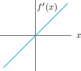
23. Indicate on the graph of the derivative function f′ in Figure 4.14 the x-values that are critical points of the function f itself. At which critical points does f have local maxima, local minima, or neither?

In Problems 24–27, the function f is defined for all x. Use the graph of f′ to decide:
(a) Over what intervals is f increasing? Decreasing?
(b) Does f have local maxima or minima? If so, which, and where?
24.
25.

26.
27.

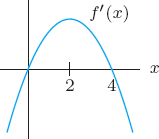
28. Figure 4.15 is a graph of f′. For what values of x does f have a local maximum? A local minimum?

Figure 4.15: Graph of f′ (not f)
29. Consumer demand for a product is changing over time, and the rate of change of demand, f′(t), in units/week, is given, in week t, for 0 ≤ t ≤ 10, in the following table.

(a) When is the demand for this product increasing? When is it decreasing?
(b) Approximately when is demand at a local maximum? A local minimum?
30. Suppose f has a continuous derivative whose values are given in the following table.
(a) Estimate the x-coordinates of critical points of f for 0 ≤ x ≤ 10.
(b) For each critical point, indicate if it is a local maximum of f, local minimum, or neither.

31. The derivative of f(t) is given by f′(t) = t3 − 6t2 + 8t for 0 ≤ t ≤ 5. Graph f′(t), and describe how the function f(t) changes over the interval t = 0 to t = 5. When is f(t) increasing and when is it decreasing? Where does f(t) have a local maximum and where does it have a local minimum?
In Problems 32–33, find constants a and b so that the minimum for the parabola f(x) = x2 + ax + b is at the given point. [Hint: Begin by finding the critical point in terms of a.]
32. (3, 5)
33. (−2, −3)
34. Find the value of a so that the function f(x) = xeax has a critical point at x = 3.
35. For what values of a and b does f(x) = a(x − b ln x) have a local minimum at the point (2, 5)? Figure 4.16 shows a graph of f(x) with a = 1 and b = 1.

36. Sketch several members of the family y = x3 − ax2 on the same axes. Discuss the effect of the parameter a on the graph. Find all critical points for this function.
37. (a) For a a positive constant, find all critical points of f(x) = x − a![]() .
.
(b) What value of a gives a critical point at x = 5? Does f(x) have a local maximum or a local minimum at this critical point?
38. Find constants a and b in the function f(x) = axebx such that f(![]() ) = 1 and the function has a local maximum at x =
) = 1 and the function has a local maximum at x = ![]() .
.
In Problems 39–41, investigate the one-parameter family of functions. Assume that a is positive.
(a) Graph f(x) using three different values for a.
(b) Using your graph in part (a), describe the critical points of f and how they appear to move as a increases.
(c) Find a formula for the x-coordinates of the critical point(s) of f in terms of a.
39. f(x) = (x − a)2
40. f(x) = x3 − ax
41. f(x) = x2e−ax
42. If m, n ≥ 2 are integers, find and classify the critical points of f(x) = xm(1 − x)n.
4.2 INFLECTION POINTS
Concavity and Inflection Points
A study of the points on the graph of a function where the slope changes sign led us to critical points. Now we will study the points on the graph where the concavity changes, either from concave up to concave down, or from concave down to concave up.
A point at which the graph of a function f changes concavity is called an inflection point of f.
The words “inflection point of f” can refer either to a point in the domain of f or to a point on the graph of f. The context of the problem will tell you which is meant.
How Do You Locate an Inflection Point?
Since the concavity of the graph of f changes at an inflection point, the sign of f″ changes there: it is positive on one side of the inflection point and negative on the other. Thus, at the inflection point, f″ is zero or undefined. (See Figure 4.17.)
Suppose f″ is defined on both sides of a point p:
- If f″ is zero or undefined at p, then p is a possible inflection point.
- To test whether p is an inflection point, check whether f″ changes sign at p.

Figure 4.17: Change in concavity (from positive to negative or vice versa) at point p
| Example 1 | Find the inflection points of f(x) = x3 − 9x2 − 48x + 52. |
| Solution | In Figure 4.18, part of the graph of f is concave up and part is concave down, so the function must have an inflection point. However, it is difficult to locate the inflection point accurately by examining the graph. To find the inflection point exactly, we calculate where the second derivative is zero. Since f′(x) = 3x2 − 18x − 48,
We can see that the graph of f(x) changes concavity at x = 3, so x = 3 is an inflection point.
Figure 4.18: Graph of f(x) = x3 − 9x2 − 48x + 52 showing the inflection point at x = 3 |

| Example 2 | Graph a function f with the following properties: f has a critical point at x = 4 and an inflection point at x = 8; the value of f′ is negative to the left of 4 and positive to the right of 4; the value of f″ is positive to the left of 8 and negative to the right of 8. |
| Solution | Since f′ is negative to the left of 4 and positive to the right of 4, the value of f(x) is decreasing to the left of 4 and increasing to the right of 4. The values of f″ tell us that the graph of f(x) is concave up to the left of 8 and concave down to the right of 8. A possible sketch is given in Figure 4.19. |

Figure 4.19: A function with a critical point at x = 4 and an inflection point at x = 8
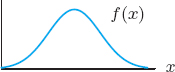
| Example 3 | Figure 4.20 shows a population growing toward a limiting population, L. There is an inflection point on the graph at the point where the population reaches L/2. What is the significance of the inflection point to the population?
Figure 4.20: Inflection point on graph of a population growing toward a limiting population, L |
| Solution | At times before the inflection point, the population is increasing faster every year. At times after the inflection point, the population is increasing slower every year. At the inflection point, the population is growing fastest. |

| Example 4 | (a) How many critical points and how many inflection points does the function f(x) = xe−x have? |
| (b) Use derivatives to find the critical points and inflection points exactly.
|
|
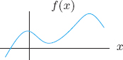
| Solution | (a) Figure 4.21 shows the graph of f(x) = xe−x. It appears to have one critical point, which is a local maximum. Are there any inflection points? Since the graph of the function is concave down at the critical point and concave up for large x, the graph of the function changes concavity, so there must be an inflection point to the right of the critical point. |
| (b) To find the critical point, find the point where the first derivative of f is zero or undefined. The product rule gives
We have f′(x) = 0 when x = 1, so the critical point is at x = 1. To find the inflection point, we find where the second derivative of f changes sign. Using the product rule on the first derivative, we have
We have f″(x) = 0 when x = 2. Since f″(x) > 0 for x > 2 and f″(x) < 0 for x < 2, the concavity changes sign at x = 2. So the inflection point is at x = 2. |

Warning!
Not every point x where f″(x) = 0 (or f″ is undefined) is an inflection point (just as not every point where f′ = 0 is a local maximum or minimum). For instance, f(x) = x4 has f″(x) = 12x2 so f″(0) = 0, but f″ > 0 when x > 0 and when x < 0, so the graph of f is concave up on both sides of x = 0. There is no change in concavity at x = 0. (See Figure 4.22.)

Figure 4.22: Graph of f(x) = x4
| Example 5 | Suppose that water is being poured into the vase in Figure 4.23 at a constant rate measured in liters per minute. Graph y = f(t), the depth of the water against time, t. Explain the concavity, and indicate the inflection points. |
| Solution | Notice that the volume of water in the vase increases at a constant rate.
At first the water level, y, rises quite slowly because the base of the vase is wide, and so it takes a lot of water to make the depth increase. However, as the vase narrows, the rate at which the water level rises increases. This means that initially y is increasing at an increasing rate, and the graph is concave up. The water level is rising fastest, so the rate of change of the depth y is at a maximum, when the water reaches the middle of the vase, where the diameter is smallest; this is an inflection point. (See Figure 4.24.) After that, the rate at which the water level changes starts to decrease, and so the graph is concave down. |


Figure 4.24: Graph of depth of water in the vase, y, against time, t
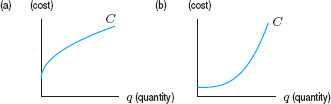
| Example 6 | What is the concavity of the graph of f(x) = ax2 + bx + c? |
| Solution | We have f′(x) = 2ax + b and f″(x) = 2a. The second derivative of f has the same sign as a. If a > 0, the graph is concave up everywhere, an upward-opening parabola. If a < 0, the graph is concave down everywhere, a downward-opening parabola. (See Figure 4.25.) If a = 0, the function is linear and the graph is a straight line. |

Problems for Section 4.2
In Problems 1–4, indicate the approximate locations of all inflection points. How many inflection points are there?
1.

2.

3.

4.

5. Graph a function with only one critical point (at x = 5) and one inflection point (at x = 10). Label the critical point and the inflection point on your graph.
6. (a) Graph a polynomial with two local maxima and two local minima.
(b) What is the least number of inflection points this function must have? Label the inflection points.
7. Graph a function which has a critical point and an inflection point at the same place.
8. During a flood, the water level in a river first rose faster and faster, then rose more and more slowly until it reached its highest point, then went back down to its pre-flood level. Consider water depth as a function of time.
(a) Is the time of highest water level a critical point or an inflection point of this function?
(b) Is the time when the water first began to rise more slowly a critical point or an inflection point?
9. When I got up in the morning I put on only a light jacket because, although the temperature was dropping, it seemed that the temperature would not go much lower. But I was wrong. Around noon a northerly wind blew up and the temperature began to drop faster and faster. The worst was around 6 pm when, fortunately, the temperature started going back up.
(a) When was there a critical point in the graph of temperature as a function of time?
(b) When was there an inflection point in the graph of temperature as a function of time?
10. For f(x) = x3 − 18x2 − 10x + 6, find the inflection point algebraically. Graph the function with a calculator or computer and confirm your answer.
11. Find the inflection points of f(x) = x4 + x3 − 3x2 + 2.
In each of Problems 12–21, use the first derivative to find all critical points and use the second derivative to find all inflection points. Use a graph to identify each critical point as a local maximum, a local minimum, or neither.
12. f(x) = x2 − 5x + 3
13. f(x) = x3 − 3x + 10
14. f(x) = 2x3 + 3x2 − 36x + 5
15. f(x) = ![]() − x + 2
− x + 2
16. f(x) = x4 − 2x2
17. f(x) = 3x4 − 4x3 + 6
18. f(x) = x4 − 8x2 + 5
19. f(x) = x4 − 4x3 + 10
20. f(x) = x5 − 5x4 + 35
21. f(x) = 3x5 − 5x3
22. (a) Use a graph to estimate the x-values of any critical points and inflection points of f(x) = e−x2.
(b) Use derivatives to find the x-values of any critical points and inflection points exactly.
23. (a) Find all critical points and all inflection points of the function f(x) = x4 − 2ax2 + b. Assume a and b are positive constants.
(b) Find values of the parameters a and b if f has a critical point at the point (2, 5).
(c) If there is a critical point at (2, 5), where are the inflection points?
24. Indicate on the graph of the derivative f′ in Figure 4.26 the x-values that are inflection points of the function f.

25. Indicate on the graph of the second derivative f″ in Figure 4.27 the x-values that are inflection points of the function f.

For Problems 26–29, sketch a possible graph of y = f(x), using the given information about the derivatives y′ = f′(x) and y″ = f″(x). Assume that the function is defined and continuous for all real x.
26.

27.


29.

30. Indicate on Figure 4.28 approximately where the inflection points of f(x) are if the graph shows
(a) The function f(x)
(b) The derivative f′(x)
(c) The second derivative f″(x)

Problems 31–34 concern f(t) in Figure 4.29, which gives the length of a human fetus as a function of its age.

31. (a) What are the units of f′(24)?
(b) What is the biological meaning of f′(24) = 1.6?
32. (a) Which is greater, f′(20) or f′(36)?
(b) What does your answer say about fetal growth?
33. (a) At what time does the inflection point occur?
(b) What is the biological significance of this point?
34. Estimate
(a) f′(20)
(b) f′(36)
(c) The average rate of change of length over the 40 weeks shown.
35. (a) Water is flowing at a constant rate (i.e., constant volume per unit time) into a cylindrical container standing vertically. Sketch a graph showing the depth of water against time.
(b) Water is flowing at a constant rate into a cone-shaped container standing on its point. Sketch a graph showing the depth of the water against time.
36. If water is flowing at a constant rate (i.e., constant volume per unit time) into the Grecian urn in Figure 4.30, sketch a graph of the depth of the water against time. Mark on the graph the time at which the water reaches the widest point of the urn.

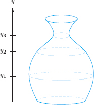
37. The vase in Figure 4.31 is filled with water at a constant rate (i.e., constant volume per unit time).
(a) Graph y = f(t), the depth of the water, against time, t. Show on your graph the points at which the concavity changes.
(b) At what depth is y = f(t) growing most quickly? Most slowly? Estimate the ratio between the growth rates at these two depths.
Find formulas for the functions described in Problems 38–40.
38. A cubic polynomial, ax3 + bx2 + cx + d, with a critical point at x = 2, an inflection point at (1,4), and a leading coefficient of 1.
39. A function of the form y = ![]() with y-intercept 2 and an inflection point at t = 1.
with y-intercept 2 and an inflection point at t = 1.
40. A curve of the form y = e−(x–a)2/b for b > 0 with a local maximum at x = 2 and points of inflection at x = 1 and x = 3.
4.3 GLOBAL MAXIMA AND MINIMA
Global Maxima and Minima
The techniques for finding maximum and minimum values make up the field called optimization. Local maxima and minima occur where a function takes larger or smaller values than at nearby points. However, we are often interested in where a function is larger or smaller than at all other points. For example, a firm trying to maximize its profit may do so by minimizing its costs. We make the following definition:
For any function f:
- f has a global minimum at p if f(p) is less than or equal to all values of f.
- f has a global maximum at p if f(p) is greater than or equal to all values of f.
How Do We Find Global Maxima and Minima?
If f is a continuous function defined on an interval a ≤ x ≤ b (including its endpoints), Figure 4.32 illustrates that the global maximum or minimum of f occurs at a local maximum or a local minimum, respectively, which could be at one of the endpoints, x = a or x = b.
To find the global maximum and minimum of a continuous function on an interval including endpoints: Compare values of the function at all the critical points in the interval and at the endpoints.
What if the continuous function is defined on an interval a < x < b (excluding its endpoints), or on the entire real line which has no endpoints? The function graphed in Figure 4.33 has no global maximum because the function has no largest value. The global minimum of this function coincides with one of the local minima and is marked. A function defined on the entire real line or on an interval excluding endpoints may or may not have a global maximum or a global minimum.
To find the global maximum and minimum of a continuous function on an interval excluding endpoints or on the entire real line: Find the values of the function at all the critical points and sketch a graph.

Figure 4.32: Global maximum and minimum on an interval domain, a ≤ x ≤ b

Figure 4.33: Global maximum and minimum on the entire real line
| Example 1 | Find the global maximum and minimum of f(x) = x3 − 9x2 − 48x + 52 on the interval −5 ≤ x ≤ 14. |
| Solution | We have calculated the critical points of this function previously using
so x = −2 and x = 8 are critical points. Since the global maxima and minima occur at a critical point or at an endpoint of the interval, we evaluate f at these four points:
Comparing these four values, we see that the global maximum is 360 and occurs at x = 14, and that the global minimum is −396 and occurs at x = 8. See Figure 4.34. |

Figure 4.34: Global maximum and minimum on the interval −5 ≤ x ≤ 14

Figure 4.35: Maximum rate of photosynthesis
| Example 2 | For time, t ≥ 0, in days, the rate at which photosynthesis takes place in the leaf of a plant, represented by the rate at which oxygen is produced, is approximated by1
When is photosynthesis occurring fastest? What is that rate? |
| Solution | To find the global maximum value of p(t), we first find critical points. We differentiate, set equal to zero, and solve for t:
Differentiating again gives
and substituting t = 20.12 gives p″(20.12) = −0.107, so t = 20.12 is a local maximum. Since t = 20.12 is the only critical point and it is a local maximum, t = 20.12 must give the global maximum. See Figure 4.35. The maximum rate is
Photosynthesis occurs fastest after about 20 days. The maximum rate is about 53.5 units of oxygen per day. |

A Graphical Example: Minimizing Gas Consumption
Next we look at an example in which a function is given graphically and the maximum and minimum values are read from a graph. We already know how to estimate the maximum and minimum values of f(x) from a graph of f(x)—read off the highest and lowest values. In this example, we see how to estimate the minimum value of the quantity f(x)/x from a graph of f(x) against x.
The question we investigate is how to set driving speeds to maximize fuel efficiency.2 We assume that gas consumption, g (in gallons/hour), as a function of velocity, v (in mph) is as shown in Figure 4.36. We want to minimize the gas consumption per mile, not the gas consumption per hour. Notice that
![]()
suggesting we minimize G = g/v.
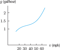
Figure 4.36: Gas consumption versus velocity
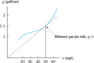
| Example 3 | Using Figure 4.36, estimate the velocity which minimizes G = g/v. |
| Solution | We want to find the minimum value of G = g/v when g and v are related by the graph in Figure 4.36. We could use Figure 4.36 to sketch a graph of G against v and estimate a critical point. But there is an easier way. Figure 4.37 shows that g/v is the slope of the line from the origin to the point P. Where on the curve should P be to make the slope a minimum? From the possible positions of the line shown in Figure 4.37, we see that the slope of the line is both a local and global minimum when the line is tangent to the curve. From Figure 4.38, we can see that the velocity at this point is about 50 mph. Thus to minimize gas consumption per mile, we should drive about 50 mph. |

Figure 4.37: Graphical representation of gas consumption per mile, G = g/v
Problems for Section 4.3
For Problems 1–2, indicate all critical points on the given graphs. Determine which correspond to local minima, local maxima, global minima, global maxima, or none of these. (Note that the graphs are on closed intervals.)
1.

2.

3. For each interval, use Figure 4.39 to choose the statement that gives the location of the global maximum and global minimum of f on the interval.
(a) 4 ≤ x ≤ 12
(b) 11 ≤ x ≤ 16
(c) 4 ≤ x ≤ 9
(d) 8 ≤ x ≤ 18
(I) Maximum at right endpoint, minimum at left end point.
(II) Maximum at right endpoint, minimum at critical point.
(III) Maximum at left endpoint, minimum at right endpoint.
(IV) Maximum at left endpoint, minimum at critical point.

In Problems 4–7, graph a function with the given properties.
4. Has local minimum and global minimum at x = 3 but no local or global maximum.
5. Has local minimum at x = 3, local maximum at x = 8, but no global maximum or minimum.
6. Has no local or global maxima or minima.
7. Has local and global minimum at x = 3, local and global maximum at x = 8.
8. True or false? Give an explanation for your answer. The global maximum of f(x) = x2 on every closed interval is at one of the endpoints of the interval.
9. Plot the graph of f(x) = x3−ex using a graphing calculator or computer to find all local and global maxima and minima for: (a) −1 ≤ x ≤ 4 (b) −3 ≤ x ≤ 2
In Problems 10–13, sketch the graph of a function on the interval 0 ≤ x ≤ 10 with the given properties.
10. Has local minimum at x = 3, local maximum at x = 8, but global maximum and global minimum at the endpoints of the interval.
11. Has local and global maximum at x = 3, local and global minimum at x = 10.
12. Has global maximum at x = 0, global minimum at x = 10, and no other local maxima or minima.
13. Has local and global minimum at x = 3, local and global maximum at x = 8.
14. The function y = t(x) is positive and continuous with a global maximum at the point (3, 3). Graph t(x) if t′(x) and t″(x) have the same sign for x < 3, but opposite signs for x > 3.
15. Figure 4.40 shows the rate at which photosynthesis is taking place in a leaf.
(a) At what time, approximately, is photosynthesis proceeding fastest for t ≥ 0?
(b) If the leaf grows at a rate proportional to the rate of photosynthesis, for what part of the interval 0 ≤ t ≤ 200 is the leaf growing? When is it growing fastest?

For the functions in Problems 16–19, do the following:
(a) Find f′ and f″.
(b) Find the critical points of f.
(c) Find any inflection points of f.
(d) Evaluate f at its critical points and at the endpoints of the given interval. Identify local and global maxima and minima of f in the interval.
(e) Graph f.
16. f(x) = x3 − 3x2 (−1 ≤ x ≤ 3)
17. f(x) = 2x3 − 9x2 + 12x + 1 (−0.5 ≤ x ≤ 3)
18. f(x) = x3 − 3x2 − 9x + 15 (−5 ≤ x ≤ 4)
19. f(x) = x + sin x (0 ≤ x ≤ 2π)
20. Find the value of x that maximizes y = 12 + 18x − 5x2 and the corresponding value of y, by
(a) Estimating the values from a graph of y.
(b) Finding the values using calculus.
21. Find the value(s) of x that give critical points of y = ax2 + bx + c, where a, b, c are constants. Under what conditions on a, b, c is the critical value a maximum? A minimum?
22. A grapefruit is tossed straight up with an initial velocity of 50 ft/sec. The grapefruit is 5 feet above the ground when it is released. Its height, in feet, at time t seconds is given by
![]()
How high does it go before returning to the ground?
23. The sum of two nonnegative numbers is 100. What is the maximum value of the product of these two numbers?
24. The product of two positive numbers is 784. What is the minimum value of their sum?
25. The sum of three nonnegative numbers is 36, and one of the numbers is twice one of the other numbers. What is the maximum value of the product of these three numbers?
26. The perimeter of a rectangle is 64 cm. Find the lengths of the sides of the rectangle giving the maximum area.
In Problems 27–32, find the exact global maximum and minimum values of the function. The domain is all real numbers unless otherwise specified.
27. g(x) = 4x − x2 − 5
28. f(x) = x + 1/x for x > 0
29. g(t) = te−t for t > 0
30. f(x) = x − ln x for x > 0
31. f(t) = ![]()
32. f(t) = (sin2 t + 2) cos t
33. What value of w minimizes S if S −5pw = 3qw2 − 6pq and p and q are positive constants?
34. The energy expended by a bird per day, E, depends on the time spent foraging for food per day, F hours. Foraging for a shorter time requires better territory, which then requires more energy for its defense.3 Find the foraging time that minimizes energy expenditure if
![]()
35. A rectangular swimming pool is to be built with an area of 1800 square feet. The owner wants 5-foot-wide decks along either side and 10-foot-wide decks at the two ends. Find the dimensions of the smallest piece of property on which the pool can be built satisfying these conditions.
36. If you have 100 feet of fencing and want to enclose a rectangular area up against a long, straight wall, what is the largest area you can enclose?
37. An apple tree produces, on average, 400 kg of fruit each season. However, if more than 200 trees are planted per km2, crowding reduces the yield by 1 kg for each tree over 200.
(a) Express the total yield, y, from one square kilometer as a function of the number of trees on it. Graph this function.
(b) How many trees should a farmer plant on each square kilometer to maximize yield?
38. On the west coast of Canada, crows eat whelks (a shell-fish). To open the whelks, the crows drop them from the air onto a rock. If the shell does not smash the first time, the whelk is dropped again.4 The average number of drops, n, needed when the whelk is dropped from a height of x meters is approximated by
![]()
(a) Give the total vertical distance the crow travels upward to open a whelk as a function of drop height, x.
(b) Crows are observed to drop whelks from the height that minimizes the total vertical upward distance traveled per whelk. What is this height?
39. During a flu outbreak in a school of 763 children, the number of infected children, I, was expressed in terms of the number of susceptible (but still healthy) children, S, by the function5
![]()
What is the maximum possible number of infected children?
40. The number of offspring in a population may not be a linear function of the number of adults. The Ricker curve, used to model fish populations, claims that y = axe−bx, where x is the number of adults, y is the number of offspring, and a and b are positive constants.
(a) Find and classify all critical points of the Ricker curve.
(b) Is there a global maximum? What does this imply about populations?
41. The oxygen supply, S, in the blood depends on the hematocrit, H, the percentage of red blood cells in the blood:
![]()
(a) What value of H maximizes the oxygen supply? What is the maximum oxygen supply?
(b) How does increasing the value of the constants a and b change the maximum value of S?
42. The quantity of a drug in the bloodstream t hours after a tablet is swallowed is given, in mg, by
![]()
(a) How much of the drug is in the bloodstream at time t = 0?
(b) When is the maximum quantity of drug in the bloodstream? What is that maximum?
(c) In the long run, what happens to the quantity?
43. When birds lay eggs, they do so in clutches of several at a time. When the eggs hatch, each clutch gives rise to a brood of baby birds. We want to determine the clutch size which maximizes the number of birds surviving to adulthood per brood. If the clutch is small, there are few baby birds in the brood; if the clutch is large, there are so many baby birds to feed that most die of starvation. The number of surviving birds per brood as a function of clutch size is shown by the benefit curve in Figure 4.41.6
(a) Estimate the clutch size which maximizes the number of survivors per brood.
(b) Suppose also that there is a biological cost to having a larger clutch: the female survival rate is reduced by large clutches. This cost is represented by the dotted line in Figure 4.41. If we take cost into account by assuming that the optimal clutch size in fact maximizes the vertical distance between the curves, what is the new optimal clutch size?

44. Let f(v) be the amount of energy consumed by a flying bird, measured in joules per second (a joule is a unit of energy), as a function of its speed v (in meters/sec). Let a(v) be the amount of energy consumed by the same bird, measured in joules per meter.
(a) Suggest a reason in terms of the way birds fly for the shape of the graph of f(v) in Figure 4.42.
(b) What is the relationship between f(v) and a(v)?
(c) Where on the graph is a(v) a minimum?
(d) Should the bird try to minimize f(v) or a(v) when it is flying? Why?

45. A person's blood pressure, p, in millimeters of mercury (mm Hg) is given, for t in seconds, by
![]()
(a) What are the maximum and minimum values of blood pressure?
(b) What is the time between successive maxima?
(c) Show your answers on a graph of blood pressure against time.
46. A chemical reaction converts substance A to substance Y. At the start of the reaction, the quantity of A present is a grams. At time t seconds later, the quantity of Y present is y grams. The rate of the reaction, in grams/sec, is given by
![]()
(a) For what values of y is the rate nonnegative? Graph the rate against y.
(b) For what values of y is the rate a maximum?
47. In a chemical reaction, substance A combines with substance B to form substance Y. At the start of the reaction, the quantity of A present is a grams, and the quantity of B present is b grams. At time t seconds after the start of the reaction, the quantity of Y present is y grams. Assume a < b and y ≤ a. For certain types of reactions, the rate of the reaction, in grams/sec, is given by
![]()
(a) For what values of y is the rate nonnegative? Graph the rate against y.
(b) Use your graph to find the value of y at which the rate of the reaction is fastest.
4.4 PROFIT, COST, AND REVENUE
Maximizing Profit
A fundamental issue for a producer of goods is how to maximize profit. For a quantity, q, the profit π(q) is the difference between the revenue, R(q), and the cost, C(q), of supplying that quantity. Thus, π(q) = R(q) − C(q). The marginal cost, MC = C′, is the derivative of C; marginal revenue is MR = R′.
Now we look at how to maximize total profit, given functions for revenue and cost. The next example suggests a criterion for identifying the optimal production level.
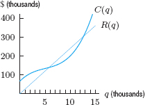
| Example 1 | Estimate the maximum profit if the revenue and cost are given by the curves R and C, respectively, in Figure 4.43.
|
| Solution | Since profit is revenue minus cost, the profit is represented by the vertical distance between the cost and revenue curves, marked by the vertical arrows in Figure 4.43. When revenue is below cost, the company is taking a loss; when revenue is above cost, the company is making a profit. The maximum profit must occur between about q = 70 and q = 200, which is the interval in which the company is making a profit. Profit is maximized when the vertical distance between the curves is largest (and revenue is above cost). This occurs at approximately q = 140.
The profit accrued at q = 140 is the vertical distance between the curves, so the maximum profit = $80,000 − $60,000 = $20,000. |

Maximum Profit Can Occur Where MR = MC
We now analyze the marginal costs and marginal revenues near the optimal point. Zooming in on Figure 4.43 around q = 140 gives Figure 4.44.
At a production level q1 to the left of 140 in Figure 4.44, marginal cost is less than marginal revenue. The company would make more money by producing more units, so production should be increased (toward a production level of 140). At any production level q2 to the right of 140, marginal cost is greater than marginal revenue. The company would lose money by producing more units and would make more money by producing fewer units. Production should be adjusted down toward 140.
What about the marginal revenue and marginal cost at q = 140? Since MC < MR to the left of 140, and MC > MR to the right of 140, we expect MC = MR at 140. In this example, profit is maximized at the point where the slopes of the cost and revenue graphs are equal.

Figure 4.44: Example 1: Maximum profit occurs where MC = MR
We can get the same result analytically. Global maxima and minima of a function can only occur at critical points of the function or at the endpoints of the interval. To find critical points of π, look for zeros of the derivative:
![]()
So
![]()
that is, the slopes of the graphs of R(q) and C(q) are equal at q. In economic language,
The maximum (or minimum) profit can occur where
![]()
that is, where
![]()
Of course, maximum or minimum profit does not have to occur where MR = MC; either one could occur at an endpoint. Example 2 shows how to visualize maxima and minima of the profit on a graph of marginal revenue and marginal cost.
| Example 2 | The total revenue and total cost curves for a product are given in Figure 4.45.
(a) Sketch the marginal revenue and marginal cost, MR and MC, on the same axes. Mark the two quantities where marginal revenue equals marginal cost. What is the significance of these two quantities? At which quantity is profit maximized? (b) Graph the profit function π(q).
|
| Solution | (a) Since R(q) is a straight line with positive slope, the graph of its derivative, MR, is a horizontal line. (See Figure 4.46.) Since C(q) is always increasing, its derivative, MC, is always positive. As q increases, the cost curve changes from concave down to concave up, so the derivative of the cost function, MC, changes from decreasing to increasing. (See Figure 4.46.) The local minimum on the marginal cost curve corresponds to the inflection point of C(q).
Where is profit maximized? We know that the maximum profit can occur when Marginal revenue = Marginal cost, that is where the curves in Figure 4.46 cross at q1 and q2. Do these points give the maximum profit? We first consider q1. To the left of q1, we have MR < MC, so π′ = MR − MC is negative and the profit function is decreasing there. To the right of q1, we have MR > MC, so π′ is positive and the profit function is increasing. This behavior, decreasing and then increasing, means that the profit function has a local minimum at q1. This is certainly not the production level we want. What happens at q2? To the left of q2, we have MR > MC, so π′ is positive and the profit function is increasing. To the right of q2, we have MR < MC, so π′ is negative and the profit function is decreasing. This behavior, increasing and then decreasing, means that the profit function has a local maximum at q2. The global maximum profit occurs either at the production level q2 or at an endpoint (the largest and smallest possible production levels). Since the profit is negative at the endpoints (see Figure 4.45), the global maximum occurs at q2.
Figure 4.46: Marginal revenue and marginal cost
(b) The graph of the profit function is in Figure 4.47. At the maximum and minimum, the slope of the profit curve is zero:
Note that since R(0) = 0 and C(0) represents the fixed costs of production, we have
Therefore the vertical intercept of the profit function is a negative number, equal in magnitude to the size of the fixed cost. |


| Example 3 | Find the quantity which maximizes profit if the total revenue and total cost (in dollars) are given by
where q is quantity and 0 ≤ q ≤ 1000 units. What production level gives the minimum profit? |
| Solution | We begin by looking for production levels that give Marginal revenue = Marginal cost. Since
MR = MC leads to
Does this represent a local maximum or minimum of the profit π? To decide, look to the left and right of 650 units. When q = 649, we have MR = $1.106 per unit, which is greater than MC = $1.10 per unit. Thus, producing one more unit (the 650th) brings in more revenue than it costs, so profit increases. When q = 651, we have M R = $1.094 per unit, which is less than M C = $1.10 per unit. It is not profitable to produce the 651st unit. We conclude that q = 650 gives a local maximum for the profit function π. To check whether q = 650 gives a global maximum, we compare the profit at the endpoints, q = 0 and q = 1000, with the profit at q = 650. At q = 0, the only cost is $300 (the fixed costs) and there is no revenue, so π(0) = −$300. At q = 1000, we have R(1000) = $2000 and C(1000) = $1400, so π(1000) = $600. At q = 650, we have R(650) = $1982.50 and C(650) = $1015, so π(650) = $967.50. Therefore, the maximum profit is obtained at a production level of q = 650 units. The minimum profit (a loss) occurs when q = 0 and there is no production at all. |


Maximizing Revenue
For some companies, costs do not depend on the number of items sold. For example, a city bus company with a fixed schedule has the same costs no matter how many people ride the buses. In such a situation, profit is maximized by maximizing revenue.
| Example 4 | At a price of $80 for a half-day trip, a white-water rafting company attracts 300 customers. Every $5 decrease in price attracts an additional 30 customers.
(a) Find the demand equation. (b) Express revenue as a function of price. (c) What price should the company charge per trip to maximize revenue? |
| Solution | (a) We first find the equation relating price to demand. If price, p, is 80, the number of trips sold, q, is 300. If p is 75, then q is 330, and so on. See Table 4.1. Because demand changes by a constant (30 people) for every $5 drop in price, q is a linear function of p. Then
so the demand equation is q = −6p + b. Since p = 80 when q = 300, we have
The demand equation is q = −6p + 780. (b) Since revenue R = p · q, revenue as a function of price is
(c) Figure 4.48 shows this revenue function has a maximum. To find it, we differentiate:
The maximum revenue is achieved when the price is $65. |

Table 4.1 Demand for rafting trips


Figure 4.48: Revenue for a rafting company as a function of price
Problems for Section 4.4
1. Figure 4.49 shows cost and revenue. For what production levels is the profit function positive? Negative? Estimate the production at which profit is maximized.
2. The revenue from selling q items is R(q) = 500q − q2, and the total cost is C(q) = 150 + 10q. Write a function that gives the total profit earned, and find the quantity which maximizes the profit.
3. Revenue is given by R(q) = 450q and cost is given by C(q) = 10,000 + 3q2. At what quantity is profit maximized? What is the total profit at this production level?
4. Using the cost and revenue graphs in Figure 4.50, sketch the following functions. Label the points q1 and q2.
(a) Total profit
(b) Marginal cost
(c) Marginal revenue

5. Figure 4.46 in Section 4.4 shows the points, q1 and q2, where marginal revenue equals marginal cost.
(a) On the graph of the corresponding total cost and total revenue functions in Figure 4.51, label the points q1 and q2. Using slopes, explain the significance of these points.
(b) Explain in terms of profit why one is a local minimum and one is a local maximum.

6. Let C(q) be the total cost of producing a quantity q of a certain product. See Figure 4.52.
(a) What is the meaning of C(0)?
(b) Describe in words how the marginal cost changes as the quantity produced increases.
(c) Explain the concavity of the graph (in terms of economics).
(d) Explain the economic significance (in terms of marginal cost) of the point at which the concavity changes.
(e) Do you expect the graph of C(q) to look like this for all types of products?

7. Let C(q) represent the cost, R(q) the revenue, and π(q) the total profit, in dollars, of producing q items.
(a) If C′(50) = 75 and R′(50) = 84, approximately how much profit is earned by the 51st item?
(b) If C′(90) = 71 and R′(90) = 68, approximately how much profit is earned by the 91st item?
(c) If π(q) is a maximum when q = 78, how do you think C′(78) and R′(78) compare? Explain.
8. Table 4.2 shows cost, C(q), and revenue, R(q).
(a) At approximately what production level, q, is profit maximized? Explain your reasoning.
(b) What is the price of the product?
(c) What are the fixed costs?

9. Table 4.3 shows marginal cost, M C, and marginal revenue, M R.
(a) Use the marginal cost and marginal revenue at a production of q = 5000 to determine whether production should be increased or decreased from 5000.
(b) Estimate the production level that maximizes profit.

10. Figure 4.53 shows graphs of marginal cost and marginal revenue. Estimate the production levels that could maximize profit. Explain your reasoning.

11. The marginal cost and marginal revenue of a company are MC(q) = 0.03q2 − 1.4q + 34 and MR(q) = 30, where q is the number of items manufactured. To increase profits, should the company increase or decrease production from each of the following levels?
(a) 25 items
(b) 50 items
(c) 80 items
12. A manufacturing process has marginal costs given in the table; the item sells for $30 per unit. At how many quantities, q, does the profit appear to be a maximum? In what intervals do these quantities appear to lie?

13. Cost and revenue functions are given in Figure 4.54. Approximately what quantity maximizes profits?

14. Cost and revenue functions are given in Figure 4.54.
(a) At a production level of q = 3000, is marginal cost or marginal revenue greater? Explain what this tells you about whether production should be increased or decreased.
(b) Answer the same questions for q = 5000.
15. When production is 2000, marginal revenue is $4 per unit and marginal cost is $3.25 per unit. Do you expect maximum profit to occur at a production level above or below 2000? Explain.
16. Revenue and cost functions for a company are given in Figure 4.55.
(a) Estimate the marginal cost at q = 400.
(b) Should the company produce the 500th item? Why?
(c) Estimate the quantity which maximizes profit.

17. A company estimates that the total revenue, R, in dollars, received from the sale of q items is R = ln(1 + 1000q2). Calculate and interpret the marginal revenue if q = 10.
18. The demand equation for a product is p = 45 − 0.01q. Write the revenue as a function of q and find the quantity that maximizes revenue. What price corresponds to this quantity? What is the total revenue at this price?
19. The demand for tickets to an amusement park is given by p = 70 − 0.02q, where p is the price of a ticket in dollars and q is the number of people attending at that price.
(a) What price generates an attendance of 3000 people? What is the total revenue at that price? What is the total revenue if the price is $20?
(b) Write the revenue function as a function of attendance, q, at the amusement park.
(c) What attendance maximizes revenue?
(d) What price should be charged to maximize revenue?
(e) What is the maximum revenue? Can we determine the corresponding profit?
20. An ice cream company finds that at a price of $4.00, demand is 4000 units. For every $0.25 decrease in price, demand increases by 200 units. Find the price and quantity sold that maximize revenue.
21. At a price of $8 per ticket, a musical theater group can fill every seat in the theater, which has a capacity of 1500. For every additional dollar charged, the number of people buying tickets decreases by 75. What ticket price maximizes revenue?
22. The demand equation for a quantity q of a product at price p, in dollars, is p = −5q + 4000. Companies producing the product report the cost, C, in dollars, to produce a quantity q is C = 6q + 5 dollars.
(a) Express a company's profit, in dollars, as a function of q.
(b) What production level earns the company the largest profit?
(c) What is the largest profit possible?
23. (a) Production of an item has fixed costs of $10,000 and variable costs of $2 per item. Express the cost, C, of producing q items.
(b) The relationship between price, p, and quantity, q, demanded is linear. Market research shows that 10,100 items are sold when the price is $5 and 12,872 items are sold when the price is $4.50. Express q as a function of price p.
(c) Express the profit earned as a function of q.
(d) How many items should the company produce to maximize profit? (Give your answer to the nearest integer.) What is the profit at that production level?
24. An online seller of knitted sweaters finds that it costs $35 to make her first sweater. Her cost for each additional sweater goes down until it reaches $25 for her 100th sweater, and after that it starts to rise again. If she can sell each sweater for $35, is the quantity sold that maximizes her profit less than 100? Greater than 100?
25. A landscape architect plans to enclose a 3000 square-foot rectangular region in a botanical garden. She will use shrubs costing $45 per foot along three sides and fencing costing $20 per foot along the fourth side. Find the minimum total cost.
26. You run a small furniture business. You sign a deal with a customer to deliver up to 400 chairs, the exact number to be determined by the customer later. The price will be $90 per chair up to 300 chairs, and above 300, the price will be reduced by $0.25 per chair (on the whole order) for every additional chair over 300 ordered. What are the largest and smallest revenues your company can make under this deal?
27. A warehouse selling cement has to decide how often and in what quantities to reorder. It is cheaper, on average, to place large orders, because this reduces the ordering cost per unit. On the other hand, larger orders mean higher storage costs. The warehouse always reorders cement in the same quantity, q. The total weekly cost, C, of ordering and storage is given by
![]()
(a) Which of the terms, a/q and bq, represents the ordering cost and which represents the storage cost?
(b) What value of q gives the minimum total cost?
28. A demand function is p = 400 − 2q, where q is the quantity of the good sold for price $p.
(a) Find an expression for the total revenue, R, in terms of q.
(b) Differentiate R with respect to q to find the marginal revenue, MR, in terms of q. Calculate the marginal revenue when q = 10.
(c) Calculate the change in total revenue when production increases from q = 10 to q = 11 units. Confirm that a one-unit increase in q gives a reasonable approximation to the exact value of MR obtained in part (b).
29. A business sells an item at a constant rate of r units per month. It reorders in batches of q units, at a cost of a + bq dollars per order. Storage costs are k dollars per item per month, and, on average, q/2 items are in storage, waiting to be sold. [Assume r, a, b, k are positive constants.]
(a) How often does the business reorder?
(b) What is the average monthly cost of reordering?
(c) What is the total monthly cost, C of ordering and storage?
(d) Obtain Wilson's lot size formula, the optimal batch size which minimizes cost.
30. (a) A cruise line offers a trip for $2000 per passenger. If at least 100 passengers sign up, the price is reduced for all the passengers by $10 for every additional passenger (beyond 100) who goes on the trip. The boat can accommodate 250 passengers. What number of passengers maximizes the cruise line's total revenue? What price does each passenger pay then?
(b) The cost to the cruise line for n passengers is 80,000+400n. What is the maximum profit that the cruise line can make on one trip? How many passengers must sign up for the maximum to be reached and what price will each pay?
31. A company manufactures only one product. The quantity, q, of this product produced per month depends on the amount of capital, K, invested (i.e., the number of machines the company owns, the size of its building, and so on) and the amount of labor, L, available each month. We assume that q can be expressed as a Cobb-Douglas production function:
![]()
where c, α, β are positive constants, with 0 < α < 1 and 0 < β < 1. In this problem we will see how the Russian government could use a Cobb-Douglas function to estimate how many people a newly privatized industry might employ. A company in such an industry has only a small amount of capital available to it and needs to use all of it, so K is fixed. Suppose L is measured in man-hours per month, and that each man-hour costs the company w rubles (a ruble is the unit of Russian currency). Suppose the company has no other costs besides labor, and that each unit of the good can be sold for a fixed price of p rubles. How many man-hours of labor per month should the company use in order to maximize its profit?
32. A company can produce and sell f(L) tons of a product per month using L hours of labor per month. The wage of the workers is w dollars per hour, and the finished product sells for p dollars per ton.
(a) The function f(L) is the company's production function. Give the units of f(L). What is the practical significance of f(1000) = 400?
(b) The derivative f′(L) is the company's marginal product of labor. Give the units of f′(L). What is the practical significance of f′(1000) = 2?
(c) The real wage of the workers is the quantity of product that can be bought with one hour's wages. Show that the real wage is w/p tons per hour.
(d) Show that the monthly profit of the company is
![]()
(e) Show that when operating at maximum profit, the company's marginal product of labor equals the real wage:
![]()
4.5 AVERAGE COST
To stay in business, a company needs to know whether it can turn a profit—which is possible if the price of its product can be set above the average cost of production.
In this section, we see how average cost can be calculated and visualized, and the relationship between average cost and marginal cost.
What Is Average Cost?
The average cost is the cost per unit of producing a certain quantity; it is the total cost divided by the number of units produced.
If the cost of producing a quantity q is C(q), then the average cost, a(q), of producing a quantity q is given by

Although both are measured in the same units, for example, dollars per item, be careful not to confuse the average cost with the marginal cost (the cost of producing the next item).
| Example 1 | A salsa company has cost function C(q) = 0.01q3 − 0.6q2 + 13q + 1000 (in dollars), where q is the number of cases of salsa produced. If 100 cases are produced, find the average cost per case. |
| Solution | The total cost of producing the 100 cases is given by
We find the average cost per case by dividing by 100, the number of cases produced.
If 100 cases of salsa are produced, the average cost is $63 per case. |
Visualizing Average Cost on the Total Cost Curve
We know that average cost is a(q) = C(q)/q. Since we can subtract zero from any number without changing it, we can write

This expression gives the slope of the line joining the points (0, 0) and (q, C(q)) on the cost curve. See Figure 4.56.

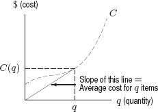
Figure 4.56: Average cost is the slope of the line from the origin to a point on the cost curve
Minimizing Average Cost
We use the graphical representation of average cost to investigate the relationship between average and marginal cost, and to identify the production level which minimizes average cost.
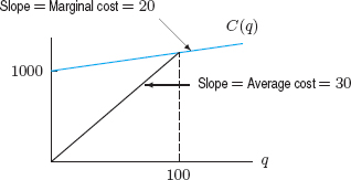
| Example 2 | A cost function, in dollars, is C(q) = 1000 + 20q, where q is the number of units produced. Find and compare the marginal cost to produce the 100th unit and the average cost of producing 100 units. Illustrate your answer on a graph. |
| Solution | The cost function is linear with fixed costs of $1000 and variable costs of $20 per unit. Thus,
This means that after 99 units have been produced, it costs an additional $20 to produce the next unit. In contrast,
Notice that the average cost includes the fixed costs of $1000 spread over the entire production, whereas marginal cost does not. Thus, the average cost is greater than the marginal cost in this example. See Figure 4.57.
|
| Example 3 | Mark on the cost graph in Figure 4.58 the quantity at which the average cost is minimized. |
| Solution | In Figure 4.59, the average costs at q1, q2, q3, and q4 are given by the slopes of the lines from the origin to the curve. These slopes are steep for small q, become less steep as q increases, and then get steeper again. Thus, as q increases, the average cost decreases and then increases, so there is a minimum value. In Figure 4.59 the minimum occurs at the point q0 where the line from the origin is tangent to the cost curve. |


Figure 4.59: Minimum average cost occurs at q0 where line is tangent to cost curve
In Figure 4.59, notice that average cost is a minimum (at q0) when average cost equals marginal cost. The next example shows what happens when marginal cost and average cost are not equal.
| Example 4 | Suppose 100 items are produced at an average cost of $2 per item. Find the average cost of producing 101 items if the marginal cost to produce the 101st item is: (a) $1 (b) $3. |
| Solution | If 100 items are produced at an average cost of $2 per item, the total cost of producing the items is 100 · $2 = $200.
(a) Since the marginal, or additional, cost to produce the 101st item is $1, the total cost of producing 101 items is $200 + $1 = $201. The average cost to produce these items is 201/101, or $1.99 per item. The average cost has gone down. (b) In this case, the marginal cost to produce the 101st item is $3. The total cost to produce 101 items is $203 and the average cost is 203/101, or $2.01 per item. The average cost has gone up. |
Notice that in Example 4(a), where it costs less than the average to produce an additional item, average cost decreases as production increases. In Example 4(b), where it costs more than the average to produce an additional item, average cost increases with production. We summarize:
Relationship Between Average Cost and Marginal Cost
- If marginal cost is less than average cost, then increasing production decreases average cost.
- If marginal cost is greater than average cost, then increasing production increases average cost.
- Marginal cost equals average cost at critical points of average cost.


| Example 6 | A total cost function, in thousands of dollars, is given by C(q) = q3 − 6q2 + 15q, where q is in thousands and 0 ≤ q ≤ 5.
(a) Graph C(q). Estimate visually the quantity at which average cost is minimized. (b) Graph the average cost function. Use it to estimate the minimum average cost. (c) Determine analytically the exact value of q at which average cost is minimized. (d) Graph the marginal cost function on the same axes as the average cost. (e) Show that at the minimum average cost, Marginal cost = Average cost. Explain how you can see this result on your graph of average and marginal costs. |
| Solution | (a) A graph of C(q) is in Figure 4.60. Average cost is minimized at the point where a line from the origin to the point on the curve has minimum slope. This occurs where the line is tangent to the curve, which is at approximately q = 3, corresponding to a production of 3000 units. |
| (b) Since average cost is total cost divided by quantity, we have
Figure 4.61 suggests that the minimum average cost occurs at q = 3. |
|
| (c) Average cost is minimized at a critical point of a(q) = q2 − 6q + 15. Differentiating gives
The minimum occurs at q = 3. |
|
| (d) See Figure 4.61. Marginal cost is the derivative of C(q) = q3 − 6q2 + 15q,
|
|
| (e) At q = 3, we have
|


Thus, marginal and average cost are equal at q = 3. This result can be seen in Figure 4.61 since the marginal cost curve cuts the average cost curve at the minimum average cost.

Figure 4.60: Cost function, showing the minimum average cost

Figure 4.61: Average and marginal cost functions, showing minimum average cost
Problems for Section 4.5
1. For each cost function in Figure 4.62, is there a value of q at which average cost is minimized? If so, approximately where? Explain your answer.
2. Figure 4.63 shows cost with q = 10,000 marked.
(a) Find the average cost when the production level is 10,000 units and interpret it.
(b) Represent your answer to part (a) graphically.
(c) At approximately what production level is average cost minimized?

3. The graph of a cost function is given in Figure 4.64.
(a) At q = 25, estimate the following quantities and represent your answers graphically.
(i) Average cost
(ii) Marginal cost
(b) At approximately what value of q is average cost minimized?

4. The cost of producing q items is C(q) = 2500 + 12q dollars.
(a) What is the marginal cost of producing the 100th item? the 1000th item?
(b) What is the average cost of producing 100 items? 1000 items?
5. The cost function is C(q) = 1000 + 20q. Find the marginal cost to produce the 200th unit and the average cost of producing 200 units.
6. Graph the average cost function corresponding to the total cost function shown in Figure 4.65.

7. The total cost of production, in thousands of dollars, is C(q) = q3 − 12q2 + 60q, where q is in thousands and 0 ≤ q ≤ 8.
(a) Graph C(q). Estimate visually the quantity at which average cost is minimized.
(b) Determine analytically the exact value of q at which average cost is minimized.
8. You are the manager of a firm that produces slippers that sell for $20 a pair. You are producing 1200 pairs of slippers each month, at an average cost of $2 each. The marginal cost at a production level of 1200 is $3 per pair.
(a) Are you making or losing money?
(b) Will increasing production increase or decrease your average cost? Your profit?
(c) Would you recommend that production be increased or decreased?
9. The average cost per item to produce q items is given by
![]()
(a) What is the total cost, C(q), of producing q goods?
(b) What is the minimum marginal cost? What is the practical interpretation of this result?
(c) At what production level is the average cost a minimum? What is the lowest average cost?
(d) Compute the marginal cost at q = 30. How does this relate to your answer to part (c)? Explain this relationship both analytically and in words.
10. The marginal cost at a production level of 2000 units of an item is $10 per unit and the average cost of producing 2000 units is $15 per unit. If the production level were increased slightly above 2000, would the following quantities increase or decrease, or is it impossible to tell?
(a) Average cost
(b) Profit
11. An agricultural worker in Uganda is planting clover to increase the number of bees making their home in the region. There are 100 bees in the region naturally, and for every acre put under clover, 20 more bees are found in the region.
(a) Draw a graph of the total number, N(x), of bees as a function of x, the number of acres devoted to clover.
(b) Explain, both geometrically and algebraically, the shape of the graph of:
(i) The marginal rate of increase of the number of bees with acres of clover, N′(x).
(ii) The average number of bees per acre of clover, N(x)/x.
12. A developer has recently purchased a laundromat and an adjacent factory. For years, the laundromat has taken pains to keep the smoke from the factory from soiling the air used by its clothes dryers. Now that the developer owns both the laundromat and the factory, she could install filters in the factory's smokestacks to reduce the emission of smoke, instead of merely protecting the laundromat from it. The cost of filters for the factory and the cost of protecting the laundromat against smoke depend on the number of filters used, as shown in the table.

(a) Make a table which shows, for each possible number of filters (0 through 7), the marginal cost of the filter, the average cost of the filters, and the marginal savings in protecting the laundromat from smoke.
(b) Since the developer wishes to minimize the total costs to both her businesses, what should she do? Use the table from part (a) to explain your answer.
(c) What should the developer do if, in addition to the cost of the filters, the filters must be mounted on a rack which costs $100?
(d) What should the developer do if the rack costs $50?
13. Show analytically that if marginal cost is less than average cost, then the derivative of average cost with respect to quantity satisfies a′(q) < 0.
14. Show analytically that if marginal cost is greater than average cost, then the derivative of average cost with respect to quantity satisfies a′(q) > 0.
15. A reasonably realistic model of a firm's costs is given by the short-run Cobb-Douglas cost curve
![]()
where a is a positive constant, F is the fixed cost, and K measures the technology available to the firm.
(a) Show that C is concave down if a > 1.
(b) Assuming that a < 1, find what value of q minimizes the average cost.
4.6 ELASTICITY OF DEMAND
The sensitivity of demand to changes in price varies with the product. For example, a change in the price of light bulbs may not affect the demand for light bulbs much, because people need light bulbs no matter what their price. However, a change in the price of a particular make of car may have a significant effect on the demand for that car, because people can switch to another make.
Elasticity of Demand
We want to find a way to measure this sensitivity of demand to price changes. Our measure should work for products as diverse as light bulbs and cars. The prices of these two items are so different that it makes little sense to talk about absolute changes in price: Changing the price of light bulbs by $1 is a substantial change, whereas changing the price of a car by $1 is not. Instead, we use the percent change in price. How, for example, does a 1% increase in price affect the demand for the product?
Let Δp denote the change in the price p of a product and Δq denote the corresponding change in quantity q demanded. The percent change in price is Δp/p and the percent change in quantity demanded is Δq/q. We assume in this book that Δp and Δq have opposite signs (because increasing the price usually decreases the quantity demanded). Then the effect of a price change on demand is measured by the absolute value of the ratio

For small changes in p, we approximate Δq/Δp by the derivative dq/dp. We define:
The elasticity of demand7 for a product, E, is given approximately by

Increasing the price of an item by 1% causes a drop of approximately E% in the quantity of goods demanded. For small changes, Δp, in price,

If E > 1, a 1% increase in price causes demand to drop by more than 1%, and we say that demand is elastic. If 0 ≤ E < 1, a 1% increase in price causes demand to drop by less than 1%, and we say that demand is inelastic. In general, a larger elasticity causes a larger percent change in demand for a given percent change in price.

| Example 2 | The demand curve for a product is given by q = 1000 − 2p2, where p is the price. Find the elasticity at p = 10 and at p = 15. Interpret your answers. |
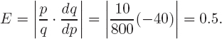
| Solution | We first find the derivative dq/dp = −4p. At a price of p = 10, we have dq/dp = −4 · 10 = −40, and the quantity demanded is q = 1000 − 2 · 102 = 800. At this price, the elasticity is
The demand is inelastic at a price of p = 10: a 1% increase in price results in approximately a 0.5% decrease in demand. At a price of $15, we have q = 550 and dq/dp = −60. The elasticity is
The demand is elastic: a 1% increase in price results in approximately a 1.64% decrease in demand. |

Revenue and Elasticity of Demand
Elasticity enables us to analyze the effect of a price change on revenue. An increase in price usually leads to a fall in demand. However, the revenue may increase or decrease. The revenue R = pq is the product of two quantities, and as one increases, the other decreases. Elasticity measures the relative significance of these two competing changes.
Elasticity allows us to predict whether revenue increases or decreases with a price increase.
| Example 4 | The item in Example 3(a) is wool whose demand equation is q = 400 − 10p. The item in Example 3(b) is houseplants, whose demand equation is q = 1300 − 100p. Find the elasticity of wool and houseplants. |
| Solution | For wool, q = 400 − 10p, so dq/dp = −10. Thus,
|
| For houseplants, q = 1300 − 100p, so dq/dp = −100. Thus,
|


Notice that EWool < 1 and revenue increases with an increase in price; EHouseplants > 1 and revenue decreases with an increase in price. In the next example we see the relationship between elasticity and maximum revenue.
| Example 5 | Table 4.4 shows the demand, q, revenue, R, and elasticity, E, for the product in Example 2 at several prices. What price brings in the greatest revenue? What is the elasticity at that price? |
| Solution | Table 4.4 suggests that maximum revenue is achieved at a price of about $13, and at that price, E is about 1. At prices below $13, we have E < 1, so the reduction in demand caused by a price increase is small; thus, raising the price increases revenue. At prices above $13, we have E > 1, so the increase in demand caused by a price decrease is relatively large; thus lowering the price increases revenue. |

Example 6 shows that revenue does have a local maximum when E = 1. We summarize as follows:
Relationship Between Elasticity and Revenue
- If E < 1, demand is inelastic and revenue is increased by raising the price.
- If E > 1, demand is elastic and revenue is increased by lowering the price.
- E = 1 occurs at critical points of the revenue function.
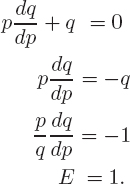
Elasticity of Demand for Different Products
Different products generally have different elasticities. See Table 4.5. If there are close substitutes for a product, or if the product is a luxury rather than a necessity, a change in price generally has a large effect on demand, and the demand for the product is elastic. On the other hand, if there are no close substitutes or if the product is a necessity, changes in price have a relatively small effect on demand, and the demand is inelastic. For example, demand for salt, penicillin, eyeglasses, and lightbulbs is inelastic over the usual range of prices for these products.
Table 4.5 Elasticity of demand (with respect to price) for selected farm products8

Problems for Section 4.6
1. The elasticity of a good is E = 0.5. What is the effect on the quantity demanded of:
(a) A 3% price increase?
(b) A 3% price decrease?
2. The elasticity of a good is E = 2. What is the effect on the quantity demanded of:
(a) A 3% price increase?
(b) A 3% price decrease?
3. What are the units of elasticity if:
(a) Price p is in dollars and quantity q is in tons?
(b) Price p is in yen and quantity q is in liters?
(c) What can you conclude in general?
4. There are many brands of laundry detergent. Would you expect the elasticity of demand for any particular brand to be high or low? Explain.
5. Would you expect the demand for high-definition television sets to be elastic or inelastic? Explain.
6. There is only one company offering local telephone service in a town. Would you expect the elasticity of demand for telephone service to be high or low? Explain.
7. What is the elasticity for peaches in Table 4.5? Explain what this number tells you about the effect of price increases on the demand for peaches. Is the demand for peaches elastic or inelastic? Is this what you expect? Explain.
8. What is the elasticity for potatoes in Table 4.5? Explain what this number tells you about the effect of price increases on the demand for potatoes. Is the demand for potatoes elastic or inelastic? Is this what you expect? Explain.
9. The demand for a product is given by q = 200 − 2p2. Find the elasticity of demand when the price is $5. Is the demand inelastic or elastic, or neither?
10. The demand for a product is given by p = 90 − 10q. Find the elasticity of demand when p = 50. If this price rises by 2%, calculate the corresponding percentage change in demand.
11. School organizations raise money by selling candy door to door. The table shows p, the price of the candy, and q, the quantity sold at that price.

(a) Estimate the elasticity of demand at a price of $1.00. At this price, is the demand elastic or inelastic?
(b) Estimate the elasticity at each of the prices shown. What do you notice? Give an explanation for why this might be so.
(c) At approximately what price is elasticity equal to 1?
(d) Find the total revenue at each of the prices shown. Confirm that the total revenue appears to be maximized at approximately the price where E = 1.
12. The demand for yams is given by q = 5000 − 10p2, where q is in pounds of yams and p is the price of a pound of yams.
(a) If the current price of yams is $2 per pound, how many pounds will be sold?
(b) Is the demand at $2 elastic or inelastic? Is it more accurate to say “People want yams and will buy them no matter what the price” or “Yams are a luxury item and people will stop buying them if the price gets too high”?
13. The demand for yams is given in Problem 12.
(a) At a price of $2 per pound, what is the total revenue for the yam farmer?
(b) Write revenue as a function of price, and then find the price that maximizes revenue.
(c) What quantity is sold at the price you found in part (b), and what is the total revenue?
(d) Show that E = 1 at the price you found in part (b).
14. It has been estimated that the elasticity of demand for slaves in the American South before the Civil War was equal to 0.86 (fairly high) in the cities and equal to 0.05 (very low) in the countryside.9
(a) Why might this be?
(b) Where do you think the staunchest defenders of slavery were from, the cities or the countryside?
15. Find the exact price that maximizes revenue for sales of the product in Example 2.
16. If E = 2 for all prices p, how can you maximize revenue?
17. If E = 0.5 for all prices p, how can you maximize revenue?
18. (a) Let p be the price and q be the quantity sold of a good with a high elasticity of demand, E. Explain intuitively (without formulas) the effect of raising the price on the revenue, R.
(b) Derive an expression for dR/dp in terms of q and E. Show all the steps and reasoning.
(c) Explain how your answer to part (b) confirms your answer to part (a).
19. (a) If the demand equation is pq = k for a positive constant k, compute the elasticity of demand.
(b) Explain the answer to part (a) in terms of the revenue function.
20. Show that a demand equation q = k/pr, where r is a positive constant, gives constant elasticity E = r.
21. If p is price and E is the elasticity of demand for a good, show analytically that
![]()
22. Suppose cost is proportional to quantity, C(q) = kq. Show that a firm earns maximum profit when
![]()
[Hint: Combine the result of Problem 21 with the fact that profit is maximized when MR = MC.]
23. A linear demand function is given in Figure 4.66. Economists compute elasticity of demand E for any quantity q0 using the formula
![]()
where d1 and d2 are the vertical distances shown in Figure 4.66.
(a) Explain why this formula works.
(b) Determine the prices, p, at which (i) E > 1 (ii) E < 1 (iii) E = 1

24. Show analytically that if elasticity of demand satisfies E > 1, then the derivative of revenue with respect to price satisfies dR/dp < 0.
25. Show analytically that if elasticity of demand satisfies E < 1, then the derivative of revenue with respect to price satisfies dR/dp > 0.
26. If q is the quantity of chicken demanded as a function of the price p of beef, the cross-price elasticity of demand for chicken with respect to the price of beef is defined as Ecross = |p/q · dq/dp|. What does Ecross tell you about the sensitivity of the quantity of chicken bought to changes in the price of beef?
27. Dwell time, t, is the time in minutes that shoppers spend in a store. Sales, s, is the number of dollars they spend in the store. The elasticity of sales with respect to dwell time is 1.3. Explain what this means in simple language.
28. Elasticity of cost with respect to quantity is defined as EC,q = q/C · dC/dq.
(a) What does this elasticity tell you about sensitivity of cost to quantity produced?
(b) Show that EC,q = Marginal cost/Average cost.
29. The income elasticity of demand for a product is defined as Eincome = |I/q · dq/dI| where q is the quantity demanded as a function of the income I of the consumer. What does Eincome tell you about the sensitivity of the quantity of the product purchased to changes in the income of the consumer?
4.7 LOGISTIC GROWTH
In 1923, eighteen koalas were introduced to Kangaroo Island, off the coast of Australia.10 The koalas thrived on the island and their population grew to about 5000 in 1997. Is it reasonable to expect the population to continue growing exponentially? Since there is only a finite amount of space on the island, the population cannot grow without bound forever. Instead we expect that there is a maximum population that the island can sustain. Population growth with an upper bound can be modeled with a logistic or inhibited growth model.
Modeling the US Population
Population projections first became important to political philosophers in the late eighteenth century. As concern for scarce resources has grown, so has the interest in accurate population projections. In the US, the population is recorded every ten years by a census. The first such census was in 1790. Table 4.6 contains the census data from 1790 to 2010.
Table 4.6 US population,11 in millions, 1790-2010


Figure 4.67: US population, 1790-1860

Figure 4.68: US population, 1790-1940
Figure 4.67 suggests that the population grew exponentially during the years 1790-1860. However, after 1860 the rate of growth began to decrease. See Figure 4.68.
The Years 1790-1860: An Exponential Model
We begin by modeling the US population for the years 1790-1860 using an exponential function. If t is the number of years since 1790 and P is the population in millions, regression gives the exponential function that fits the data as approximately12
![]()
Thus, between 1790 and 1860, the US population was growing at an annual rate of about 3%.
The function P = 3.9(1.03)t is plotted in Figure 4.69 with the data; it fits the data remarkably well. Of course, since we used the data from throughout the 70-year period, we should expect good agreement throughout that period. What is surprising is that if we had used only the populations in 1790 and 1800 to create our exponential function, the predictions would still be very accurate. It is amazing that a person in 1800 could predict the population 60 years later so accurately, especially when one considers all the wars, recessions, epidemics, additions of new territory, and immigration that took place from 1800 to 1860.

Figure 4.69: An exponential model for the US population, 1790-1860

Figure 4.70: The exponential model and the US population, 1790-1940. Not a good fit beyond 1860
The Years 1790-1940: A Logistic Model
How well does the exponential function fit the US population beyond 1860? Figure 4.70 shows a graph of the US population from 1790 until 1940 with the exponential function P = 3.9(1.03)t. The exponential function which fit the data so well for the years 1790-1860 does not fit very well beyond 1860. We must look for another way to model this data.
The graph of the function given by the data in Figure 4.68 is concave up for small values of t, but then appears to become concave down and to be leveling off. This kind of growth is modeled with a logistic function. If t is in years since 1790, the function
![]()
which is graphed in Figure 4.71, fits the data well up to 1940. Such a formula is found by logistic regression on a calculator or computer.13

Figure 4.71: A logistic model for US population, 1790-1940
The Logistic Function
A logistic function, such as that used to model the US population, is everywhere increasing. Its graph is concave up at first, then becomes concave down, and levels off at a horizontal asymptote. As we saw in the US population model, a logistic function is approximately exponential for small14 values of t. A logistic function can be used to model the sales of a new product and the spread of a virus.
For positive constants L, C, and k, a logistic function has the form
![]()
The general logistic function has three parameters: L, C, and k. In Example 1, we investigate the effect of two of these parameters on the graph; Problem 2 at the end of the section considers the third.
| Example 1 | Consider the logistic function (a) Let k = 1. Graph P for several values for L. Explain the effect of the parameter L. (b) Now let L = 1. Graph P for several values for k. Explain the effect of the parameter k. |
| Solution | (a) See Figure 4.72. Notice that the graph levels off at the value L. The parameter L determines the horizontal asymptote and the upper bound for P.
Figure 4.72: Graph of
|
| (b) See Figure 4.73. Notice that as k increases, the curve approaches the asymptote more rapidly. The parameter k affects the steepness of the curve. |


The Carrying Capacity and the Point of Diminishing Returns
Example 1 suggests that the parameter L of the logistic function is the value at which P levels off, where
![]()
This value L is called the carrying capacity and represents the largest population an environment can support.
One way to estimate the carrying capacity is to find the inflection point. The graph of a logistic curve is concave up at first and then concave down. At the inflection point, where the concavity changes, the slope is largest. To the left of this point, the graph is concave up and the rate of growth is increasing. To the right of this point, the graph is concave down and the rate of growth is diminishing. The inflection point is called the point of diminishing returns. Problem 70 in the Review Problems shows that this point is at P = L/2. See Figure 4.74. Companies sometimes watch for this concavity change in the sales of a new product and use it to estimate the maximum potential sales.
Properties of the logistic function ![]() :
:
- The limiting value L represents the carrying capacity for P.
- The point of diminishing returns is the inflection point where P is growing the fastest. It occurs where P = L/2.
- The logistic function is approximately exponential for small values of t, with growth rate k.

The Years 1790-2010: Another Look at the US Population
We used a logistic function to model the US population between 1790 and 1940. How well does this model fit the US population since 1940? We now look at all the population data from 1790 to 2010.
| Example 2 | If t is in years since 1790 and P is in millions, we used the following logistic function to model the US population between 1790 and 1940:
According to this function, what is the maximum US population? Is this prediction accurate? How well does this logistic model fit the growth of the US population since 1940? Table 4.7 Predicted versus actual US population, in millions, 1940-2010 (logistic model)
|
| Solution | Table 4.7 shows the actual US population between 1940 and 2010 and the predicted values using this logistic model. According to the formula for the logistic function, the upper bound for the population is L = 192 million. However, Table 4.7 shows that the actual US population was above this figure by 1970. The fit between the logistic function and the actual population is not a good one beyond 1940. See Figure 4.75. |


Figure 4.75: The logistic model and the US population, 1790-2010
Despite World War II, which depressed population growth between 1942 and 1945, in the last half of the 1940s the US population surged. The 1950s saw a population growth of 28 million, leaving our logistic model in the dust. This surge in population is referred to as the baby boom.
Once again we have reached a point where our model is no longer useful. This should not lead you to believe that a reasonable mathematical model cannot be found; rather, it points out that no model is perfect and that when one model fails, we seek a better one. Just as we abandoned the exponential model in favor of the logistic model for the US population, we could look further.
Sales Predictions
Total sales of a new product often follow a logistic model. For example, when a new application (app) for a mobile device comes on the market, sales first increase rapidly as word of the app spreads. Eventually, most of the people who want the app have already bought it and sales slow down. The graph of total sales against time is concave up at first and then concave down, with the upper bound L equal to the maximum potential sales.
| Example 3 | Table 4.8 shows the total sales (in thousands) of new app since it was introduced.
(a) Find the point where concavity changes in this function. Use it to estimate the maximum potential sales, L. (b) Using logistic regression, fit a logistic function to this data. What maximum potential sales does this function predict? |
| Solution | (a) The rate of change of total sales increases until t = 5 and decreases after t = 5, so the inflection point is at approximately t = 5, when P = 258. So L/2 = 258 and L = 516. The maximum potential sales for this app are estimated to be 516,000. |
| (b) Logistic regression gives the following function:
Maximum potential sales predicted by this function are L = 532, or about 532,000. See Figure 4.76. |
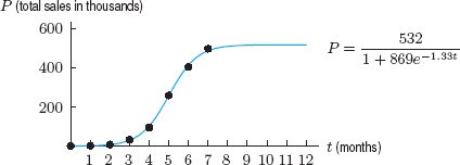
Dose-Response Curves
A dose-response curve plots the intensity of physiological response to a drug as a function of the dose administered. As the dose increases, the intensity of the response increases, so a dose-response function is increasing. The intensity of the response is generally scaled as a percentage of the maximum response. The curve cannot go above the maximum response (or 100%), so the curve levels off at a horizontal asymptote. Dose-response curves are generally concave up for low doses and concave down for high doses. A dose-response curve can be modeled by a logistic function with the independent variable being the dose of the drug, not time.
A dose-response curve shows the amount of drug needed to produce the desired effect, as well as the maximum effect attainable and the dose required to obtain it. The slope of the dose-response curve gives information about the therapeutic safety margin of the drug.
Drugs need to be administered in a dose which is large enough to be effective but not so large as to be dangerous. Figure 4.77 shows two different dose-response curves: one with a small slope and one with a large slope. In Figure 4.77(a), there is a broad range of dosages at which the drug is both safe and effective. In Figure 4.77(b), where the slope of the curve is steep, the range of dosages at which the drug is both safe and effective is small. If the slope of the dose-response curve is steep, a small mistake in the dosage can have dangerous results. Administration of such a drug is difficult.

Figure 4.77: What does the slope of the dose-response curve tell us?
| Example 4 | Figure 4.78 shows dose-response curves for three different drugs used for the same purpose. Discuss the advantages and disadvantages of the three drugs.
Figure 4.78: What are the advantages and disadvantages of each of these drugs? |
| Solution | Drugs A and B show the same maximum response, both above the maximum safe level. Drug A reaches this level more quickly. The maximum response of Drug C is significantly lower, while still reaching the minimum desired level. Thus, Drug C may be the preferred drug despite its lower maximum effect because it is the safest to administer. |

Problems for Section 4.7
1. If t is in years since 1990, one model for the population of the world, P, in billions, is
![]()
(a) What does this model predict for the maximum sustainable population of the world?
(b) Graph P against t.
(c) According to this model, when will the earth's population reach 20 billion? 39.9 billion?
2. Investigate the effect of the parameter C on the logistic curve
![]()
Substitute several values for C and explain, with a graph and with words, the effect of C on the graph.
3. The following table shows the total sales, in thousands, since a new game was brought to market.
(a) Plot this data and mark on your plot the point of diminishing returns.
(b) Predict total possible sales of this game, using the point of diminishing returns.

4. Write a paragraph explaining why sales of a new product often follow a logistic curve. Explain the benefit to the company of watching for the point of diminishing returns.
5. (a) Draw a logistic curve. Label the carrying capacity L and the point of diminishing returns t0.
(b) Draw the derivative of the logistic curve. Mark the point t0 on the horizontal axis.
(c) A company keeps track of the rate of sales (for example, sales per week) rather than total sales. Explain how the company can tell on a graph of rate of sales when the point of diminishing returns is reached.
6. The following table gives the percentage, P, of households with cable television between 1977 and 2003.15

(a) Explain why a logistic model is reasonable for this data.
(b) Estimate the point of diminishing returns. What limiting value L does this point predict? Does this limiting value appear to be accurate, given the percentages for 2002 and 2003?
(c) If t is in years since 1977, the best fitting logistic function for this data turns out to be
![]()
What limiting value does this function predict?
(d) Explain in terms of percentages of households what the limiting value is telling you. Do you think your answer to part (c) is an accurate prediction?
7. The Tojolobal Mayan Indian community in Southern Mexico has available a fixed amount of land.16 The proportion, P, of land in use for farming t years after 1935 is modeled with the logistic function
![]()
(a) What proportion of the land was in use for farming in 1935?
(b) What is the long-run prediction of this model?
(c) When was half the land in use for farming?
(d) When is the proportion of land used for farming increasing most rapidly?
8. In the spring of 2003, SARS (Severe Acute Respiratory Syndrome) spread rapidly in several Asian countries and Canada. Table 4.9 gives the total number, P, of SARS cases reported in Hong Kong17 by day t, where t = 0 is March 17, 2003.
(a) Find the average rate of change of P for each interval in Table 4.9.
(b) In early April 2003, there was fear that the disease would spread at an ever-increasing rate for a long time. What is the earliest date by which epidemiologists had evidence to indicate that the rate of new cases had begun to slow?
(c) Explain why an exponential model for P is not appropriate.
(d) It turns out that a logistic model fits the data well. Estimate the value of t at the inflection point. What limiting value of P does this point predict?
(e) The best-fitting logistic function for this data turns out to be
![]()
What limiting value of P does this function predict?
Table 4.9 Total number of SARS cases in Hong Kong by day t (where t = 0 is March 17, 2003)

9. Substitute t = 0, 10, 20, . . . , 70 into the exponential function used in this section to model the US population 1790–1860. Compare the predicted values of the population with the actual values.
10. On page 214, a logistic function was used to model the US population. Use this function to predict the US population in each of the census years from 1790–1940. Compare the predicted and actual values.
11. A curve representing the total number of people, P, infected with a virus often has the shape of a logistic curve of the form
![]()
with time t in weeks. Suppose that 10 people originally have the virus and that in the early stages the number of people infected is increasing approximately exponentially, with a continuous growth rate of 1.78. It is estimated that, in the long run, approximately 5000 people will become infected.
(a) What should we use for the parameters k and L?
(b) Use the fact that when t = 0, we have P = 10, to find C.
(c) Now that you have estimated L, k, and C, what is the logistic function you are using to model the data? Graph this function.
(d) Estimate the length of time until the rate at which people are becoming infected starts to decrease. What is the value of P at this point?
12. Find the point where the following curve is steepest:
![]()
13. A dose-response curve is given by R = f(x), where R is percent of maximum response and x is the dose of the drug in mg. The curve has the shape shown in Figure 4.77. The inflection point is at (15, 50) and f′(15) = 11.
(a) Explain what f′(15) tells you in terms of dose and response for this drug.
(b) Is f′(10) greater than or less than 11? Is f′(20) greater than or less than 11? Explain.
14. If R is percent of maximum response and x is dose in mg, the dose-response curve for a drug is given by
![]()
(a) Graph this function.
(b) What dose corresponds to a response of 50% of the maximum? This is the inflection point, at which the response is increasing the fastest.
(c) For this drug, the minimum desired response is 20% and the maximum safe response is 70%. What range of doses is both safe and effective for this drug?
15. Dose-response curves for three different products are given in Figure 4.79.
(a) For the desired response, which drug requires the largest dose? The smallest dose?
(b) Which drug has the largest maximum response? The smallest?
(c) Which drug is the safest to administer? Explain.

16. Explain why it is safer to use a drug for which the derivative of the dose-response curve is smaller.
There are two kinds of dose-response curves. One type, discussed in this section, plots the intensity of response against the dose of the drug. We now consider a dose-response curve in which the percentage of subjects showing a specific response is plotted against the dose of the drug. In Problems 17–18, the curve on the left shows the percentage of subjects exhibiting the desired response at the given dose, and the curve on the right shows the percentage of subjects for which the given dose is lethal.
17. In Figure 4.80, what range of doses appears to be both safe and effective for 99% of all patients?

18. In Figure 4.81, discuss the possible outcomes and what percent of patients fall in each outcome when 50 mg of the drug is administered.

19. A population, P, growing logistically is given by
![]()
(a) Show that
![]()
(b) Explain why part (a) shows that the ratio of the additional population the environment can support to the existing population decays exponentially.
20. Cell membranes contain ion channels. The fraction, f, of channels that are open is a function of the membrane potential V (the voltage inside the cell minus voltage outside), in millivolts (mV), given by
![]()
(a) Find the values of L, k, and C in the logistic formula for f:
![]()
(b) At what voltages V are 10%, 50% and 90% of the channels open?
4.8 THE SURGE FUNCTION AND DRUG CONCENTRATION
Nicotine in the Blood
When a person smokes a cigarette, the nicotine from the cigarette enters the body through the lungs, is absorbed into the blood, and spreads throughout the body. Most cigarettes contain between 0.5 and 2.0 mg of nicotine; approximately 20% (between 0.1 and 0.4 mg) is actually inhaled and absorbed into the person's bloodstream. As the nicotine leaves the blood, the smoker feels the need for another cigarette. The half-life of nicotine in the bloodstream is about two hours. The lethal dose is considered to be about 60 mg.
The nicotine level in the blood rises as a person smokes, and tapers off when smoking ceases. Table 4.10 shows blood nicotine concentration (in ng/ml) during and after the use of cigarettes. (Smoking occurred during the first ten minutes and the experimental data shown represent average values for ten people.)18
The points in Table 4.10 are plotted in Figure 4.82. Functions with this behavior are called surge functions. They have equations of the form y = ate−bt, where a and b are positive constants.
Table 4.10 Blood nicotine concentrations during and after the use of cigarettes
![]()

Figure 4.82: Blood nicotine concentrations during and after the use of cigarettes

Figure 4.83: One member of the family y = ate−bt, with a = 1 and b = 1
The Family of Functions y = ate−bt
What effect do the positive parameters a and b have on the shape of the graph of y = ate−bt? Start by looking at the graph with a = 1 and b = 1. See Figure 4.83. We consider the effect of the parameter b on the graph of y = ate−bt now; the parameter a is considered in Problem 2 of this section.
The Effect of the Parameter b on y = te−bt
Graphs of y = te−bt for different positive values of b are shown in Figure 4.84. The general shape of the curve does not change as b changes, but as b decreases, the curve rises for a longer period of time and to a higher value.

Figure 4.84: Graph of y = te−bt, with b varying

Figure 4.85: How does the maximum depend on b?
We see in Figure 4.85 that, when b = 1, the maximum occurs at about t = 1. When b = 2, it occurs at about t = ![]() , and when b = 3, it occurs at about t =
, and when b = 3, it occurs at about t = ![]() . The next example shows that the maximum of the function y = te−bt occurs at t = 1/b.
. The next example shows that the maximum of the function y = te−bt occurs at t = 1/b.

The surge function y = ate−bt, for positive constants a and b, increases rapidly and then decreases toward zero with a maximum at t = 1/b. See Figure 4.86.

Figure 4.86: Curve showing drug concentration as a function of time
Drug Concentration Curves
As with nicotine, the graph of concentration against time is called the drug concentration curve. If t is the time since the drug was administered, the concentration, C, can be modeled by the surge function C = ate−bt, where a and b are positive constants. (See Figure 4.86.)
Factors Affecting Drug Absorption
Drug interactions and the age of the patient can affect the drug concentration curve. In Problems 11 and 13, we see that food intake can also affect the rate of absorption of a drug, and (perhaps most surprising) that drug concentration curves can vary markedly between different commercial versions of the same drug.
| Example 2 | Figure 4.87 shows the drug concentration curves for paracetamol (acetaminophen) alone and for paracetamol taken in conjunction with propantheline. Figure 4.88 shows drug concentration curves for patients known to be slow absorbers of the drug, for paracetamol alone and for paracetamol in conjunction with metoclopramide. Discuss the effects of the additional drugs on peak concentration and the time to reach peak concentration.19
Figure 4.87: Drug concentration curves for paracetamol, normal patients
Figure 4.88: Drug concentration curves for paracetamol, patients with slow absorption |
| Solution | Figure 4.87 shows it takes about 1.5 hours for the paracetamol to reach its peak concentration, and that the maximum concentration reached is about 23 μg of paracetamol per ml of blood. However, if propantheline is administered with the paracetamol, it takes much longer to reach the peak concentration (about three hours, or approximately double the time), and the peak concentration is much lower, at about 16 μg/ml.
Comparing the curves for paracetamol alone in Figures 4.87 and 4.88 shows that the time to reach peak concentration is the same (about 1.5 hours), but the maximum concentration is lower for patients with slow absorption. When metoclopramide is given with paracetamol in Figure 4.88, the peak concentration is reached faster and is higher. |


Minimum Effective Concentration
The minimum effective concentration of a drug is the blood concentration necessary to achieve a pharmacological response. The time at which this concentration is reached is referred to as onset; termination occurs when the drug concentration falls below this level. See Figure 4.89.

Figure 4.89: When is the drug effective?
| Example 3 | Depo-Provera was approved for use in the US in 1992 as a contraceptive. Figure 4.90 shows the drug concentration curve for a dose of 150 mg given intramuscularly.20 The minimum effective concentration is about 4 ng/ml. How often should the drug be administered?
Figure 4.90: Drug concentration curve for Depo-Provera
|
| Solution | The minimum effective concentration on the drug concentration curve is plotted as a dotted horizontal line at 4 ng/ml. See Figure 4.91. We see that the drug becomes effective almost immediately and ceases to be effective after about four months. Doses should be given about every four months.
Although the dosage interval is four months, notice that it takes ten months after injections are discontinued for Depo-Provera to be entirely eliminated from the body. Fertility during that period is unpredictable. |


Problems for Section 4.8
1. If time, t, is in hours and concentration, C, is in ng/ml, the drug concentration curve for a drug is given by
![]()
(a) Graph this curve.
(b) How many hours does it take for the drug to reach its peak concentration? What is the concentration at that time?
(c) If the minimum effective concentration is 10 ng/ml, during what time period is the drug effective?
(d) Complications can arise whenever the level of the drug is above 4 ng/ml. How long must a patient wait before being safe from complications?
2. Let b = 1, and graph C = ate−bt using different values for a. Explain the effect of the parameter a.
3. If t is in hours, the drug concentration curve for a drug is given by C = 17.2te−0.4t ng/ml. The minimum effective concentration is 10 ng/ml.
(a) If the second dose of the drug is to be administered when the first dose becomes ineffective, when should the second dose be given?
(b) If you want the onset of effectiveness of the second dose to coincide with termination of effectiveness of the first dose, when should the second dose be given?
4. Figure 4.92 shows drug concentration curves for anhydrous ampicillin for newborn babies and adults.21 Discuss the differences between newborns and adults in the absorption of this drug.

5. Absorption of different forms of the antibiotic erythromycin may be increased, decreased, delayed or not affected by food. Figure 4.93 shows the drug concentration levels of erythromycin in healthy, fasting human volunteers who received single oral doses of 500 mg erythromycin tablets, together with either large (250 ml) or small (20 ml) accompanying volumes of water.22 Discuss the effect of the water on the concentration of erythromycin in the blood. How are the peak concentration and the time to reach peak concentration affected? When does the effect of the volume of water wear off?

6. Hydrocodone bitartrate is a cough suppressant usually administered in a 10 mg oral dose. The peak concentration of the drug in the blood occurs 1.3 hours after consumption and the peak concentration is 23.6 ng/ml. Draw the drug concentration curve for hydrocodone bitartrate.
7. Figure 4.82 shows the concentration of nicotine in the blood during and after smoking a cigarette. Figure 4.94 shows the concentration of nicotine in the blood during and after using chewing tobacco or nicotine gum. (The chewing occurred during the first 30 minutes and the experimental data shown represent the average values for ten patients.)23 Compare the three nicotine concentration curves (for cigarettes, chewing tobacco and nicotine gum) in terms of peak concentration, the time until peak concentration, and the rate at which the nicotine is eliminated from the bloodstream.

8. If t is in minutes since the drug was administered, the concentration, C(t) in ng/ml, of a drug in a patient's bloodstream is given by
![]()
(a) How long does it take for the drug to reach peak concentration? What is the peak concentration?
(b) What is the concentration of the drug in the body after 15 minutes? After an hour?
(c) If the minimum effective concentration is 10 ng/ml, when should the next dose be administered?
9. For time t ≥ 0, the function C = ate−bt with positive constants a and b gives the concentration, C, of a drug in the body. Figure 4.95 shows the maximum concentration reached (in nanograms per milliliter, ng/ml) after a 10 mg dose of the cough medicine hydrocodone bitartrate. Find the values of a and b.
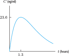
10. This problem shows how a surge can be modeled with a difference of exponential decay functions.
(a) Using graphs of e−t and e−2t, explain why the graph of f(t) = e−t − e−2t has the shape of a surge.
(b) Find the critical point and inflection point of f.
11. Figure 4.96 shows the plasma levels of canrenone in a healthy volunteer after a single oral dose of spironolactone given on a fasting stomach and together with a standardized breakfast. (Spironolactone is a diuretic agent that is partially converted into canrenone in the body.)24 Discuss the effect of food on peak concentration and time to reach peak concentration. Is the effect of the food strongest during the first 8 hours, or after 8 hours?

12. The method of administering a drug can have a strong influence on the drug concentration curve. Figure 4.97 shows drug concentration curves for penicillin following various routes of administration. Three milligrams per kilogram of body weight were dissolved in water and administered intravenously (IV), intramuscularly (IM), subcutaneously (SC), and orally (PO). The same quantity of penicillin dissolved in oil was administered intramuscularly (P-IM). The minimum effective concentration (MEC) is labeled on the graph.25
(a) Which method reaches peak concentration the fastest? The slowest?
(b) Which method has the largest peak concentration? The smallest?
(c) Which method wears off the fastest? The slowest?
(d) Which method has the longest effective duration? The shortest?
(e) When penicillin is administered orally, for approximately what time interval is it effective?

13. Figure 4.98 shows drug concentration curves after oral administration of 0.5 mg of four digoxin products. All the tablets met current USP standards of potency, disintegration time, and dissolution rate.26
(a) Discuss differences and similarities in the peak concentration and the time to reach peak concentration.
(b) Give possible values for minimum effective concentration and maximum safe concentration that would make Product C or Product D the preferred drug.
(c) Give possible values for minimum effective concentration and maximum safe concentration that would make Product A the preferred drug.

14. Figure 4.99 shows a graph of the percentage of drug dissolved against time for four tetracycline products A, B, C, and D. Figure 4.100 shows the drug concentration curves for the same four tetracycline products.27 Discuss the effect of dissolution rate on peak concentration and time to reach peak concentration.


CHAPTER SUMMARY
- Using the first derivative
Critical points, local maxima and minima
- Using the second derivative
Inflection points, concavity
- Optimization
Global maxima and minima
- Maximizing profit and revenue
- Average cost
Minimizing average cost
- Elasticity
- Families of functions
Parameters. The surge function, drug concentration curves. The logistic function, carrying capacity, point of diminishing returns.
REVIEW PROBLEMS FOR CHAPTER FOUR
For Problems 1–2, indicate all critical points on the given graphs. Which correspond to local minima, local maxima, global maxima, global minima, or none of these? (Note that the graphs are on closed intervals.)
1.

2.

In Problems 3–7, use derivatives to find the critical points and inflection points.
3. f(x) = x3 − 9x2 + 24x + 5
4. f(x) = x5 − 10x3 − 8
5. f(x) = x5 + 15x4 + 25
6. f(x) = 5x − 3 ln x
7. f(x) = 4xe3x
In Problems 8–9, find the value(s) of x for which:
(a) f(x) has a local maximum or local minimum. Indicate which ones are maxima and which are minima.
(b) f(x) has a global maximum or global minimum.
8. f(x) = x10 − 10x, and 0 ≤ x ≤ 2
9. f(x) = x − ln x, and 0.1 ≤ x ≤ 2
10. (a) Find the critical points of p(1 − p)4.
(b) Classify the critical points as local maxima, local minima, or neither.
(c) What are the maximum and minimum values of p(1 − p)4 on 0 ≤ x ≤ 1?
11. On July 1, the price of a stock had a critical point. How could the price have been changing during the time around July 1?
12. (a) Show that if a is a positive constant, then x = 0 is the only critical point of f(x) = x + a![]() .
.
(b) Use derivatives to show that f is increasing and its graph is concave down for all x > 0.
13. On the graph of f′ in Figure 4.101, indicate the x-values that are critical points of the function f itself. Are they local maxima, local minima, or neither?

Figure 4.101: Graph of f′ (not f)
Problems 14–15 show the graph of a derivative function f′. Indicate on a sketch the x-values that are critical points of the function f itself. Identify each critical point as a local maximum, a local minimum, or neither.
14.

15.

16. Suppose f has a continuous derivative. From the values of f′ (θ) in the following table, estimate the θ values with 1 < θ < 2.1 at which f(θ) has a local maximum or minimum. Identify which is which.

17. (a) Find the derivative of f(x) = x5 + x + 7. What is its sign?
(b) How many real roots does the equation x5 + x + 7 = 0 have? How do you know?
[Hint: How many critical points does this function have?]
18. (a) If b is a positive constant and x > 0, find all critical points of f(x) = x − b ln x.
(b) Use the second-derivative test to determine whether the function has a local maximum or local minimum at each critical point.
19. If a and b are nonzero constants, find the domain and all critical points of
![]()
20. (a) On a computer or calculator, graph f(θ) = θ − sin θ. Can you tell whether the function has any zeros in the interval 0 ≤ θ ≤ 1?
(b) Find f′. What does the sign of f′ tell you about the zeros of f in the interval 0 ≤ θ ≤ 1?
21. For the function, f, graphed in Figure 4.102:
(a) Sketch f′(x).
(b) Where does f′(x) change its sign?
(c) Where does f′(x) have local maxima or minima?

22. Using your answer to Problem 21 as a guide, write a short paragraph (using complete sentences) which describes the relationships between the following features of a function f:
- The local maxima and minima of f.
- The points at which the graph of f changes concavity.
- The sign changes of f′.
- The local maxima and minima of f′.
23. The graphs of f(x) = 1 + e−ax for a = 1, 2, and 5, are in Figure 4.103. Without a calculator, identify the graphs by looking at f′(0).
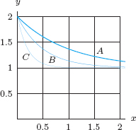
24. The graphs of f(x) = xe−ax for a = 1, 2, and 3, are in Figure 4.104. Without a calculator, identify the graphs by locating the critical points of f(x).

25. If water is flowing at a constant rate (i.e., constant volume per unit time) into the vase in Figure 4.105, sketch a graph of the depth of the water against time. Mark on the graph the time at which the water reaches the corner of the vase.

26. Water flows at a constant rate into the left side of the W-shaped container in Figure 4.106. Sketch a graph of the height, H, of the water in the left side of the container as a function of time, t. The container starts empty.

27. In 1774, Captain James Cook left 10 rabbits on a small Pacific island. The rabbit population is approximated by
![]()
with t measured in years since 1774. Using a calculator or computer:
(a) Graph P. Does the population level off?
(b) Estimate when the rabbit population grew most rapidly. How large was the population at that time?
(c) Find the inflection point on the graph and explain its significance for the rabbit population.
(d) What natural causes could lead to the shape of the graph of P?
28. The polynomial f has exactly two local maxima and one local minimum; these are the only critical points of f.
(a) Sketch a possible graph of f.
(b) What is the largest number of zeros f could have?
(c) What is the smallest number of zeros f could have?
(d) What is the smallest number of inflection points f could have?
(e) What is the smallest degree f could have?
(f) Find a possible formula for f(x).
29. For f(x) = sin(x2) between x = 0 and x = 3, find the coordinates of all intercepts, critical points, and inflection points to two decimal points.
30. (a) Graph f(x) = x + a sin x for a = 0.5 and a = 3.
(b) For what values of a is f(x) increasing for all x?
31. (a) Graph f(x) = x2 + a sin x for a = 1 and a = 20.
(b) For what values of a is f(x) concave up for all x?
32. Figure 4.107 gives the derivative of g(x) on −2 ≤ x ≤ 2.
(a) Write a few sentences describing the behavior of g(x) on this interval.
(b) Does the graph of g(x) have any inflection points? If so, give the approximate x-coordinates of their locations. Explain your reasoning.
(c) What are the global maxima and minima of g on [−2, 2]?
(d) If g(−2) = 5, what do you know about g(0) and g(2)? Explain.

33. For some positive constant C, a patient's temperature change, T, due to a dose, D, of a drug is given by
![]()
(a) What dosage maximizes the temperature change?
(b) The sensitivity of the body to the drug is defined as dT/dD. What dosage maximizes sensitivity?
34. A rectangle has one side on the x-axis and two corners on the top half of the circle of radius 1 centered at the origin. Find the maximum area of such a rectangle. What are the coordinates of its vertices?
35. A closed box has a fixed surface area A and a square base with side x.
(a) Find a formula for its volume, V, as a function of x.
(b) Sketch a graph of V against x.
(c) Find the maximum value of V.
36. As an epidemic spreads through a population, the number of infected people, I, is expressed as a function of the number of susceptible people, S, by
![]()
(a) Find the maximum number of infected people.
(b) The constant k is a characteristic of the particular disease; the constants S0 and I0 are the values of S and I when the disease starts. Which of the following affects the maximum possible value of I? Explain.
- The particular disease, but not how it starts.
- How the disease starts, but not the particular disease.
- Both the particular disease and how it starts.
37. The hypotenuse of a right triangle has one end at the origin and one end on the curve y = x2e−3x, with x ≥ 0. One of the other two sides is on the x-axis, the other side is parallel to the y-axis. Find the maximum area of such a triangle. At what x-value does it occur?
In Problems 38–39 a vertical line divides a region into two pieces. Find the value of the coordinate x that maximizes the product of the two areas.
38.

39.

40. Which point on the curve y = ![]() is closest to the origin?
is closest to the origin?
41. Find the point(s) on the ellipse
![]()
(a) Closest to the point (2, 0).
(b) Closest to the focus (![]() , 0).
, 0).
[Hint: Minimize the square of the distance—this avoids square roots.]
42. What are the dimensions of the closed cylindrical can that has surface area 280 square centimeters and contains the maximum volume?
43. The following table gives the cost and revenue, in dollars, for different production levels, q.
(a) At approximately what production level is profit maximized?
(b) What price is charged per unit for this product?
(c) What are the fixed costs of production?

44. Figure 4.108 gives cost and revenue. What are fixed costs? What quantity maximizes profit, and what is the maximum profit earned?

45. Marginal revenue and marginal cost are given in the following table. Estimate the production levels that could maximize profit. Explain.

46. Figure 4.109 shows cost and revenue for a product.
(a) Estimate the production level that maximizes profit.
(b) Graph marginal revenue and marginal cost for this product on the same axes. Label on this graph the production level that maximizes profit.

47. The marginal revenue and marginal cost for a certain item are graphed in Figure 4.110. Do the following quantities maximize profit for the company? Explain your answer.
(a) q = a
(b) q = b
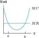
48. The total cost of producing q units of a product is given by C(q) = q3 − 60q2 + 1400q + 1000 for 0 ≤ q ≤ 50; the product sells for $788 per unit. What production level maximizes profit? Find the total cost, total revenue, and total profit at this production level. Graph the cost and revenue functions on the same axes, and label the production level at which profit is maximized and the corresponding cost, revenue, and profit. [Hint: Costs can go as high as $46,000.]
49. The total cost C(q) of producing q goods is given by:
![]()
(a) What is the fixed cost?
(b) What is the maximum profit if each item is sold for $7? (Assume you sell everything you produce.)
(c) Suppose exactly 34 goods are produced. They all sell when the price is $7 each, but for each $1 increase in price, 2 fewer goods are sold. Should the price be raised, and if so by how much?
50. The demand equation for a product is p = b1 − a1q and the cost function is C(q) = b2 + a2q, where p is the price of the product and q is the quantity sold. Find the value of q, in terms of the positive constants b1, a1, b2, a2, that maximizes profit.
51. A manufacturer's cost of producing a product is given in Figure 4.111. The manufacturer can sell the product for a price p each (regardless of the quantity sold), so that the total revenue from selling a quantity q is R(q) = pq.
(a) The difference π(q) = R(q) − C(q) is the total profit. For which quantity q0 is the profit a maximum? Mark your answer on a sketch of the graph.
(b) What is the relationship between p and C′(q0)? Explain your result both graphically and analytically. What does this mean in terms of economics? (Note that p is the slope of the line R(q) = pq. Note also that π(q) has a maximum at q = q0, so π′(q0) = 0.)
(c) Graph C′(q) and p (as a horizontal line) on the same axes. Mark q0 on the q-axis.

52. Let C(q) = 0.04q3 − 3q2 + 75q + 96 be the total cost of producing q items.
(a) Find the average cost per item as a function of q.
(b) Use a graphing calculator or computer to graph average cost against q.
(c) For what values of q is the average cost per item decreasing? Increasing?
(d) For what value of q is the average cost per item smallest? What is the smallest average cost per item at that point?
53. Graph a cost function where the minimum average cost of $25 per unit is achieved by producing 15,000 units.
54. Figure 4.112 shows the cost, C(q), and the revenue, R(q), for a quantity q. Label the following points on the graph:
(a) The point F representing the fixed costs.
(b) The point B representing the break-even level of production.
(c) The point M representing the level of production at which marginal cost is a minimum.
(d) The point A representing the level of production at which average cost a(q) = C(q)/q is a minimum.
(e) The point P representing the level of production at which profit is a maximum.

In Problems 55–60, cost, C(q), is a positive, increasing, concave-down function of quantity produced, q. Which one of the two numbers is the larger?
55. C′(2) and C′(3)
56. C′(5) and ![]()
57. ![]()
58. ![]()
59. C′(3) and C(3)/3
60. C(10)/10 and C(25)/25
61. The demand for a product is q = 2000 − 5p where q is units sold at a price of p dollars. Find the elasticity if the price is $20, and interpret your answer in terms of demand.
62. Each of the graphs in Figure 4.113 belongs to one of the following families of functions. In each case, identify which family is most likely:
an exponential function,
a logarithmic function,
a polynomial (What is the degree? Is the leading coefficient positive or negative?),
a logistic function,
a surge function.

63. Find the dimensions of the rectangle with perimeter 200 meters that has the largest area.
64. A square-bottomed box with a top has a fixed volume, V. What dimensions minimize the surface area?
65. A right triangle has one vertex at the origin and one vertex on the curve y = e−x/3 for 1 ≤ x ≤ 5. One of the two perpendicular sides is along the x-axis; the other is parallel to the y-axis. Find the maximum and minimum areas for such a triangle.
66. A line goes through the origin and a point on the curve y = x2e−3x, for x ≥ 0. Find the maximum slope of such a line. At what x-value does it occur?
67. A rectangle has one side on the x-axis, one side on the y-axis, one vertex at the origin and one on the curve y = e−2x for x ≥ 0. Find the
(a) Maximum area
(b) Minimum perimeter
68. A pigeon is released from a boat (point B in Figure 4.114) floating on a lake. Because of falling air over the cool water, the energy required to fly one meter over the lake is twice the corresponding energy e required for flying over the bank (e = 3 joule/meter). To minimize the energy required to fly from B to the loft, L, the pigeon heads to a point P on the bank and then flies along the bank to L. The distance ![]() is 2000 m, and
is 2000 m, and ![]() is 500 m. The angle at A is a right angle.
is 500 m. The angle at A is a right angle.
(a) Express the energy required to fly from B to L via P as a function of the angle θ (the angle BPA).
(b) What is the optimal angle θ?
(c) Does your answer change if ![]() ,
, ![]() and e have different numerical values?
and e have different numerical values?

69. The bell-shaped curve of statistics has formula
![]()
where μ is the mean and σ is the standard deviation.
(a) Where does p(x) have a maximum?
(b) Does p(x) have a point of inflection? If so, where?
70. Consider a population P satisfying the logistic equation
![]()
(a) Use the chain rule to find d2P/dt2.
(b) Show that the point of diminishing returns, where d2P/dt2 = 0, occurs where P = L/2.
71. Let C = ate−bt represent a drug concentration curve.
(a) Discuss the effect on peak concentration and time to reach peak concentration of varying the parameter a while keeping b fixed.
(b) Discuss the effect on peak concentration and time to reach peak concentration of varying the parameter b while keeping a fixed.
(c) Suppose a = b, so C = ate−at. Discuss the effect on peak concentration and time to reach peak concentration of varying the parameter a.
72. The rate of sales of an automobile anti-theft device are given in the following table.
(a) When is the point of diminishing returns reached?
(b) What are the total sales at this point?
(c) Assuming logistic sales growth, use your answer to part (b) to estimate total potential sales of the device.

73. Figure 4.115 shows the concentration of bemetizide (a diuretic) in the blood after single oral doses of 25 mg alone, or 25 mg bemetizide and 50 mg triamterene in combination.28 If the minimum effective concentration in a patient is 40 ng/ml, compare the effect of combining bemetizide with triamterene on peak concentration, time to reach peak concentration, time until onset of effectiveness, and duration of effectiveness. Under what circumstances might it be wise to use the triamterene with the bemetizide?

74. The distance, s, traveled by a cyclist, who starts at 1 pm, is given in Figure 4.116. Time, t, is in hours since noon.
(a) Explain why the quantity s/t is represented by the slope of a line from the origin to the point (t, s) on the graph.
(b) Estimate the time at which the quantity s/t is a maximum.
(c) What is the relationship between the quantity s/t and the instantaneous speed of the cyclist at the time you found in part (b)?

75. A bird such as a starling feeds worms to its young. To collect worms, the bird flies to a site where worms are to be found, picks up several in its beak, and flies back to its nest. The loading curve in Figure 4.117 shows how the number of worms (the load) a starling collects depends on the time it has been searching for them.29 The curve is concave down because the bird can pick up worms more efficiently when its beak is empty; when its beak is partly full, the bird becomes much less efficient. The traveling time (from nest to site and back) is represented by the distance PO in Figure 4.117. The bird wants to maximize the rate at which it brings worms to the nest, where
![]()
(a) Draw a line in Figure 4.117 whose slope is this rate.
(b) Using the graph, estimate the load which maximizes this rate.
(c) If the traveling time is increased, does the optimal load increase or decrease? Why?

76. Table 4.11 shows the total number of cars in a University of Arizona parking lot at 30-minute intervals.30
(a) Graph the total number of cars in the parking lot as a function of time. Estimate the capacity of the parking lot, and when it was full.
(b) Construct a table, and then plot a graph, of the rate of arrival of cars as a function of time.
(c) From your graph in part (b), estimate when rush hour occurred.
(d) Explain the relationship between the points on the graphs in parts (a) and (b) where rush hour occurred.
Table 4.11 Total number of cars, C, at time t
![]()
77. A single cell of a bee's honey comb has the shape shown in Figure 4.118. The surface area of this cell is given by

where h, s, θ are as shown in the picture.
(a) Keeping h and s fixed, for what angle, θ, is the surface area a minimum?
(b) Measurements on bee's cells have shown that the angle actually used by bees is about θ = 55°. Comment.

78. An organism has size W at time t. For positive constants A, b, and c, the Gompertz growth function gives
![]()
(a) Find the intercepts and asymptotes.
(b) Find the critical points and inflection points.
(c) Graph W for various values of A, b, and c.
(d) A certain organism grows fastest when it is about 1/3 of its final size. Would the Gompertz growth function be useful in modeling its growth? Explain.
STRENGTHEN YOUR UNDERSTANDING
In Problems 1–80, indicate whether the statement is true or false.
1. The function f has a local maximum at p if f(p) ≤ f(x) for points x near p.
2. If f′(p) = 0 then p is a critical point of f.
3. If p is a critical point of f then f′(p) = 0.
4. If f is increasing at all points to the left of p and decreasing at all points to the right of p then f has a local maximum at p.
5. If f′(p) = 0 and f″(p) > 0 then f has a local maximum at p.
6. If f′(p) = 0 and f″(p) > 0 then f has a local minimum at p.
7. If f″(p) > 0 then f has a local minimum at p.
8. Every critical point of f is either a local maximum or local minimum of f.
9. A function f must have at least one critical point.
10. If f has a local minimum at x = p then f′(p) = 0.
11. A point at which a graph changes concavity is called an inflection point.
12. If f″(p) = 0 then p is an inflection point of f.
13. A point p can be both a critical point and an inflection point of a function f.
14. The function f(x) = x3 has an inflection point at x = 0.
15. The function H(x) = x4 has an inflection point at x = 0.
16. A function f can have one inflection point and no critical points.
17. A function f can have 2 critical points and 3 inflection points.
18. If f″(x) = x(x + 1) then f has an inflection point at x = −1.
19. If f″(x) = x(x + 1)2 then f has an inflection point at x = −1.
20. If f″(x) = ex(x + 1) then f has an inflection point at x = −1. is an inflection point.
21. A local maximum of f can also be a global maximum of f.
22. A global maximum of f on the interval 1 ≤ x ≤ 2 always occurs at a critical point.
23. Every function has a global minimum.
24. If function y = f(x) is increasing on the interval a ≤ x ≤ b, then the global maximum of f on this interval occurs at x = b.
25. If a function y = f(x) has f′(x) < 0 for all x in the interval a ≤ x ≤ b, then the global maximum of f on this interval occurs at x = b.
26. A function S(x) could have a different global maximum on each of the intervals 1 ≤ x ≤ 2 and 2 ≤ x ≤ 3.
27. The function k(x) = 1/x has a global maximum when x > 0.
28. The function f has a global maximum on the interval −5 ≤ x ≤ 5 at p if f(p) ≤ f(x) for all −5 ≤ x ≤ 5.
29. The function f has a global minimum on the interval −5 ≤ x ≤ 5 at p if f(p) ≤ f(x) for all −5 ≤ x ≤ 5.
30. If f′(p) = 0 and f″(p) > 0 then p is a global minimum of f.
31. If marginal cost is less than marginal revenue, then increasing quantity sold will increase profit.
32. If marginal cost is greater than marginal revenue, then decreasing quantity sold will increase profit.
33. When marginal revenue equals marginal cost there is maximum profit.
34. If revenue is greater than cost, profit is the vertical distance between the cost and revenue curves.
35. Maximum profit occurs at a critical point of the cost function.
36. Maximum profit can occur when marginal profit is zero.
37. Profit is maximized where the cost and revenue curves cross.
38. Profit is zero where the graphs of the cost and revenue curves cross.
39. If prices are constant, the graph of marginal revenue is a horizontal line.
40. If prices are constant, the graph of revenue is a horizontal line.
41. Average cost is total cost for q items divided by q.
42. Marginal cost and average cost have the same units.
43. Marginal cost is the same thing as average cost.
44. The average cost of q items is the slope of the tangent line to the cost curve at q.
45. If marginal cost is less than average cost, increasing production increases average cost.
46. Marginal cost equals average cost at critical points of marginal cost.
47. If marginal cost is greater than average cost, then increasing production increases average cost.
48. Average cost has a critical point at a quantity where the line from the origin to the cost curve is also tangent to the cost curve.
49. Average cost is a decreasing function of quantity.
50. Marginal and average cost functions are both minimized at the same quantity.
51. The elasticity of demand is given by E = |q/p · dq/dp|.
52. If elasticity, E, is greater than one, then demand is inelastic.
53. If elasticity, E, is such that 0 ≤ E < 1 then demand is elastic.
54. Elasticity is a measure of the effect on demand of a change in price.
55. If a product is considered a necessity, the demand is generally elastic.
56. An increase in price always causes an increase in revenue.
57. If elasticity E > 1 then revenue increases when price increases.
58. At a critical point of the revenue function, demand is neither elastic nor inelastic.
59. If elasticity E < 1 then profit increases with an increase in price.
60. An increase in price always causes an increase in profit.
61. If P = 1000/(1 + 2e−3t) then P is a logistic function.
62. If P = 1000/(1 + 2e3t) then P is a logistic function.
63. The function P = 1000/(1 + 2e−3t) has an inflection point when t = 500.
64. The function P = 1000/(1 + 2e−3t) has an inflection point when P = 500.
65. The logistic function P = L/(1 + Ce−kt) approaches L as t increases.
66. If the slope of the dose/response curve is large, a small change in the dose will have a large effect on the response.
67. The carrying capacity of a population growing logistically is the largest population the environment can support.
68. The parameter k in the logistic function P = L/(1 + Ce−kt) affects the rate at which the curve approaches its asymptote L.
69. The logistic function P = L/(1 + Ce−kt) is concave up for P < L/2.
70. The logistic function P = L/(1 + Ce−kt) is always increasing.
71. The surge function is an exponential decay function.
72. The surge function has one critical point, which is a global maximum.
73. The surge function is always concave down.
74. If minimum effective concentration is positive and less than peak concentration, then the surge function will intersect the minimum effective concentration line at two points.
75. If minimum effective concentration is greater than peak concentration, then the drug will be effective only for the first half of the time interval.
76. The surge function has exactly one inflection point, and it is always at a t-value greater than the t-value of the critical point.
77. The minimum effective concentration of a drug is the blood concentration necessary to achieve a specific pharmacologic response.
78. The function y = t/(12e3t) is a surge function.
79. The function y = t/(12e−3t) is a surge function.
80. The surge function y = 5te−3t has maximum at t = 1/3.
PROJECTS FOR CHAPTER FOUR
1. Average and Marginal Costs
The total cost of producing a quantity q is C(q). The average cost a(q) is given in Figure 4.119. The following rule is used by economists to determine the marginal cost C′(q0), for any q0:
- Construct the tangent line t1 to a(q) at q0.
- Let t2 be the line with the same vertical intercept as t1 but with twice the slope of t1.
Then C′(q0) is the vertical distance shown in Figure 4.119. Explain why this rule works.

2. Firebreaks
The summer of 2000 was devastating for forests in the western US: over 3.5 million acres of trees were lost to fires, making this the worst fire season in 30 years. This project studies a fire management technique called firebreaks, which reduce the damage done by forest fires. A firebreak is a strip where trees have been removed in a forest so that a fire started on one side of the strip will not spread to the other side. Having many firebreaks helps confine a fire to a small area. On the other hand, having too many firebreaks involves removing large swaths of trees.31
(a) A forest in the shape of a 50 km by 50 km square has firebreaks in rectangular strips 50 km by 0.01 km. The trees between two firebreaks are called a stand of trees. All firebreaks in this forest are parallel to each other and to one edge of the forest, with the first firebreak at the edge of the forest. The firebreaks are evenly spaced throughout the forest. (For example, Figure 4.120 shows four firebreaks.) The total area lost in the case of a fire is the area of the stand of trees in which the fire started plus the area of all the firebreaks.

(i) Find the number of firebreaks that minimizes the total area lost to the forest in the case of a fire.
(ii) If a firebreak is 50 km by b km, find the optimal number of firebreaks as a function of b. If the width, b, of a firebreak is quadrupled, how does the optimal number of firebreaks change?
(b) Now suppose firebreaks are arranged in two equally spaced sets of parallel lines, as shown in Figure 4.121. The forest is a 50 km by 50 km square, and each firebreak is a rectangular strip 50 km by 0.01 km. Find the number of firebreaks in each direction that minimizes the total area lost to the forest in the case of a fire.

3. Production and the Price of Raw Materials
The production function f(x) gives the number of units of an item that a manufacturing company can produce from x units of raw material. The company buys the raw material at price w dollars per unit and sells all it produces at a price of p dollars per unit. The quantity of raw material that maximizes profit is denoted by x*.
(a) Do you expect the derivative f′(x) to be positive or negative? Justify your answer.
(b) Explain why the formula π(x) = pf(x) − wx gives the profit π(x) that the company earns as a function of the quantity x of raw materials that it uses.
(d) Assuming it is nonzero, is f″(x*) positive or negative?
(e) If the supplier of the raw materials is likely to change the price w, then it is appropriate to treat x* as a function of w. Find a formula for the derivative dx*/dw and decide whether it is positive or negative.
(f) If the price w goes up, should the manufacturing company buy more or less of the raw material?
4. Medical Case Study: Impact of Asthma on Breathing32
Asthma is a common breathing disease in which inflammation in the airways of the lungs causes episodes of shortness of breath, coughing, and chest tightness. Patients with asthma often have wheezing, an abnormal sound heard on exhalation due to turbulent airflow. Turbulent airflow is caused by swelling, mucus secretion, and constriction of muscle in the walls of the airways, shrinking the radius of the air passages leading to increased resistance to airflow and making it harder for patients to exhale.
An important breathing test for asthma is called spirometry. In this test, a patient takes in as deep a breath as he or she can, and then exhales as rapidly, forcefully, and for as long as possible through a tube connected to an analyzer. The analyzer measures a number of parameters and generates two graphs.
(a) Figure 4.122 is a volume-time curve for an asthma-free patient, showing the volume of air exhaled, V, as a function of time, t, since the test began.33
(i) What is the physical interpretation of the slope of the volume-time curve?
(ii) The volume VC shown on the volume-time graph is called the (forced) vital capacity (FVC or simply VC). Describe the physical meaning of VC.
(b) Figure 4.123 is the flow-volume curve for the same patient.34 The flow-volume curve shows the flow rate, dV/dt, of air as a function of V, the volume of air exhaled.
(i) What is the physical interpretation of the slope of the flow-volume curve?
(ii) Describe how the slope of the flow-volume curve changes as V increases from 0 to 5.5 liters. Explain what this means for the patient's breath.
(iii) Sketch the slope of the flow-volume curve.
(iv) What is the volume of air that has been exhaled when the flow rate is a maximum, and what is that maximal rate, the peak expiratory flow? Explain how this maximal rate is identified on the flow-volume curve and how the volume at which the maximal rate occurs is identified on the slope curve in part (b)(iii).
(c) How do you imagine the volume-time curve and the flow-volume curve would be different for a patient with acute asthma? Draw curves to illustrate your thinking.
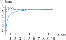
Figure 4.122: Volume-time curve

Figure 4.123: Flow-volume curve
1Examples adapted from Rodney Gentry, Introduction to Calculus for the Biological and Health Sciences (Reading: Addison-Wesley, 1978).
2Adapted from Peter D. Taylor, Calculus: The Analysis of Functions (Toronto: Wall & Emerson, 1992).
3Adapted from Graham Pyke, reported by J. R. Krebs and N. B. Davis in An Introduction to Behavioural Ecology (Oxford: Blackwell, 1987).
4Adapted from Reto Zach, reported by J. R. Krebs and N. B. Davis in An Introduction to Behavioural Ecology (Oxford: Blackwell, 1987).
5Data from Communicable Disease Surveillance Centre (UK), reported in “Influenza in a Boarding School”, British Medical Journal, March 4, 1978.
6Data from C. M. Perrins and D. Lack, reported by J. R. Krebs and N. B. Davies in An Introduction to Behavioural Ecology (Oxford: Blackwell, 1987).
7When it is necessary to distinguish it from other elasticities, this quantity is called the elasticity of demand with respect to price, or the price elasticity of demand.
8Estimated by the US Department of Agriculture and reported in W. Adams & J. Brock, The Structure of American Industry, 10th ed (Englewood Cliffs: Prentice Hall, 2000).
9Donald McCloskey, The Applied Theory of Price, p. 134 (New York: Macmillan, 1982).
10Watertown Daily Times, April 18, 1997.
11www.census.gov. Accessed February 12, 2012.
12See Appendix A: Fitting Formulas to Data. Different algorithms may give different formulas.
13See Appendix A: Fitting Formulas to Data.
14Just how small is small enough depends on the values of the parameters C and k.
15The World Almanac and Book of Facts 2005, p. 310 (New York).
16Adapted from J. S. Thomas and M. C. Robbins, “The Limits to Growth in a Tojolobal Maya Ejido,” Geoscience and Man 26, pp. 9–16 (Baton Rouge: Geoscience Publications, 1988).
17www.who.int/csr/country/en, accessed July 13, 2003.
18Benowitz, Porched, Skeiner, Jacog, “Nicotine Absorption and Cardiovascular Effects with Smokeless Tobacco Use: Comparison with Cigarettes and Nicotine Gum,” Clinical Pharmacology and Therapeutics 44 (1988): 24.
19Graeme S. Avery, ed. Drug Treatment: Principle and Practice of Clinical Pharmacology and Therapeutics (Sydney: Adis Press, 1976).
20Robert M. Julien, A Primer of Drug Action (W. H. Freeman and Co, 1995).
21Pediatrics, 1973, 51, 578.
22J. W. Bridges and L.F. Chasseaud, Progress in Drug Metabolism (New York: John Wiley and Sons, 1980).
23Benowitz, Porchet, Skeiner, Jacob, “Nicotine Absorption and Cardiovascular Effects with Smokeless Tobacco Use: Comparison with Cigarettes and Nicotine Gum,” Clinical Pharmacology and Therapeutics 44 (1988): 24.
24Welling & Tse, Pharmacokinetics of Cardiovascular, Central Nervous System, and Antimicrobial Drugs (The Royal Society of Chemistry, 1985).
25J. W. Bridges and L. F. Chasseaud, Progress in Drug Metabolism (New York: John Wiley and Sons, 1980).
26Graeme S. Avery, ed. Drug Treatment: Principles and Practice of Clinical Pharmacology and Therapeutics (Sydney: Adis Press, 1976).
27J. W. Bridges and L.F. Chasseaud, Progress in Drug Metabolism (New York: John Wiley and Sons, 1980).
28Welling & Tse, Pharmacokinetics of Cardiovascular, Central Nervous System, and Antimicrobial Drugs (The Royal Society of Chemistry, 1985).
29Alex Kacelnick (1984). Reported by J. R. Krebs and N. B. Davis, An Introduction to Behavioural Ecology (Oxford: Blackwell, 1987).
30Adapted from Nancy Roberts et al., Introduction to Computer Simulation, p. 93 (Reading: Addison-Wesley, 1983).
31Adapted from D. Quinney and R. Harding, Calculus Connections (New York: John Wiley & Sons, 1996).
32From David E. Sloane, M.D.
33Image based on www.aafp.org/afp/2004/0301/p1107.html, accessed July 9, 2011.
34Image from http://www.aafp.org/afp/2004/0301/p1107.html, accessed July 9, 2011.