13

SAP Data Warehouse Cloud and SAP Analytics Cloud

In the previous chapter, we discussed SAP HANA Cloud as the managed offering of HANA that can be used as the database runtime for data modeling and HANA native development.

We will continue our data-to-value journey and learn about the data management solutions built on top of SAP HANA and how they can help translate enterprise data into business insights.

In this chapter, we will focus on the following topics:

• SAP Data Warehouse Cloud (DWC)
• SAP Analytics Cloud (SAC)

Through this chapter, you will learn about the advanced modeling capabilities and collaboration that are provided through a virtualized workspace called Space in SAP DWC, as well as data visualization, Business Intelligence (BI), and augmented analytics in SAC.

Let’s get started!

Technical requirements

To experiment with SAP DWC, you will require an SAP BTP trial account. An SAP DWC trial tenant can be requested at https://www.sap.com/products/data-warehouse-cloud/trial.html, while an SAC trial tenant can be requested at https://www.sap.com/products/cloud-analytics/trial.html.

SAP Data Warehouse Cloud (DWC)

Before we introduce what SAP DWC is, first, let’s understand the differences between a data lake and a data warehouse.

A data lake is a data repository that holds a large amount of raw data in its natural format, often coming from disparate sources, including a mix of structured, semi-structured (CSV, XML, and JSON), and unstructured data formats. It offers an effective solution for collecting and storing large amounts of data but doesn’t necessarily need to process it until it is required for use.

In contrast, data warehousing has a more focused use case that is optimized to store and transform large amounts of data for advanced queries and analytics in a more structured relational database. It has two key functions: it acts as a federated repository of business data, and then as the query execution and processing engine of the data. The goal of a modern data warehouse is to gain insights from data. To support that, it usually includes building blocks such as the following:

• Data preparation
• A global semantic layer
• Governance and policy
• Data integration with various data sources, including data lakes

SAP DWC is an offering in the cloud that’s designed for both technical and business users to provide modern and unified data modeling and warehousing as a service that enables users to integrate, transform, model, and gain insights from data.

Collaborations in DWC are enabled through a virtual workspace called Space so that the different departments can work on the same datasets, with necessary isolation and security policies defined at each Space level. DWC separates the data layer and business layer. With the data layer, data engineers can create their models with a technical approach; the business layer empowers business users to easily drag and drop to model and explore data.

As it is built on top of SAP HANA Cloud, the broad data management capabilities discussed in the previous chapter are supported in DWC as well. Besides this, you can benefit from its cloud qualities as a fully managed offering, such as high frequency of releases, ease of use, high availability and reliability, and low maintenance effort.

Use cases

SAP DWC allows you to converge data from SAP and non-SAP applications into a fully managed cloud environment that helps simplify the data warehousing landscape. It supports a variety of use cases, such as the following scenarios:

• As the enterprise data warehouse consolidates data across cloud and on-premise environments, it reuses data models from on-premise SAP Business Warehouse (BW) with built-in SQL and data transformation capabilities and acts as the acceleration layer for BI use cases.
• It enables self-service data modeling for business users with an intuitive drag-and-drop UI fully governed by the IT department. Business semantic modeling is separated from data modeling and physical data storage.
• It democratizes enterprise data by utilizing pre-built business content from SAP and partners to support end-to-end business scenarios and speed up time to insights.
• It enables a true collaboration model around the data through cross-space collaboration and data sharing and extends the reach to more data for various industries and lines of business (LoB), such as through Data Marketplace.
• It provides seamless integration with SAC for advanced analytics and visualizations.

Next, let’s explore another concept of SAP DWC, space.

Understanding Space

Space is one of the key concepts in SAP DWC. Spaces are essentially isolated virtual environments, but collaboration can be achieved through sharing across spaces, which allows the different departments to have their own spaces, such as between LoBs and IT.

Working with data in DWC means creating a Space or accessing an existing Space. Each Space is allocated a certain amount of disk and memory storage that can be specified when it is created. DWC follows the same data tiering concept as SAP HANA Cloud.

The status of all Space storage utilization is shown on the Space Management page, with a color-coding system of red, green, or blue to indicate the resource usage. It is important to keep an eye on Space usage. When a Space exceeds its quota, it can be locked and operations such as creating new models are not allowed. In that case, you can delete unwanted data or increase the Space’s quota to unlock the Space. You can also configure the workload classes by specifying the priority of a Space range from 0 (lowest) to 8 (highest). From a job scheduling perspective, statements in a higher-priority Space will be executed first. The default priority is five; priority nine is reserved for system operations.

DWC also provides a command-line interface (CLI) (@sap/dwc-cli) to automate the management of Spaces. You can use the CLI to create, read, update, or delete a Space, assign members, update Space properties, and more. Here is an example of creating a space: $ dwc spaces create -H <Server_URL> -p <Passcode> -f </path/to/definition/file.json>.

More information about @sap/dwc-cli can be found at https://www.npmjs.com/package/@sap/dwc-cli.

DWC maintains access rights by assigning roles to users. Within DWC, only one user can be assigned as the System Owner, who has full access to all application areas. A user with the Administrator role has full privilege for the entire DWC tenant, such as creating users and spaces, creating custom roles, and assigning them to other users. A Space Administrator has full access to a Space and can create the data access controls of a Space, as well as leverage the Content Network to import pre-delivered contents into a Space. There are other roles with fewer permissions, such as the Integrator role, which can manage the data connections, create database users, and connect HDI containers with Spaces. A Modeler can manage objects through the Data Builder and Business Builder areas of a Space, while Viewers only have read access to objects in a Space.

Connectivity and data integration

SAP DWC provides various options for integrating and ingesting data from a wide variety of sources, for both SAP and non-SAP data sources. DWC runs on top of the HANA Cloud database, so it can benefit from the data integration options of HANA Cloud such as Smart Data Access (SDA) and Smart Data Integration (SDI). You can also write data to the Space through its Open SQL schema and associate it with data artifacts in an HDI container. SDI also provides additional integration options to non-SAP data sources through its Data Provisioning Agent and adaptors. Besides this, you can leverage the SAP BW metadata and data through SAP BW Bridge. Now, let’s have a look at these data integration options.

Access to the HANA database

Sometimes, you may want to work directly with the underlying HANA Cloud database of DWC to leverage its advanced capabilities; for example, using HANA machine learning libraries. In that case, you will need to create a database user as an Administrator, which is a technical user that can be used to connect with the underlying HANA database.

For each database user, an Open SQL schema is created. An Open SQL shema used to connect with your SQL clients, which can be granted write access to perform DDL and DML operations, such as ingesting data into a DWC.

You can also run the DWC-specific stored procedure known as "DWC_GLOBAL"."GRANT_PRIVILEGE_TO_SPACE" to grant write privilege to the individual tables. DWC users can always read data in the Open SQL schema for modeling in Data Builder. For read access, the database user can also read the data from a Space through the Space Schema if the data has been exposed.

If you already have data in an HDI Container or want to consume the data and models in your Space from your existing HDI container, you can create an SAP support ticket to map the HDI container with the DWC Space. Once mapped, objects in the HDI container are available in Data Builder; this scenario is referred to as HDI Ingestion. Instead, you can access Space objects in the HDI container, which is referred to as the HDI Consumption scenario.

To use HANA machine learning libraries (APL and PAL) in DWC, the HANA Script Server must be enabled for the underlying HANA database. At the time of writing, you will need to create an SAP support ticket to create the database user with the required authorizations.

Connecting with SAP HANA Cloud, data lake

To access a large amount of data, you can connect a DWC Space to SAP HANA Cloud, data lake. You will also need to create an SAP support ticket to associate the data lake with a DWC tenant. At the time of writing, only one Space of a DWC tenant can be assigned to access the data lake.

Once connected, the tables in the data lake can be accessed in DWC via the virtual tables in the Open SQL schema. DWC provides two stored procedures to create and access the tables in the data lake:

• Uses the "DWC_GLOBAL"."DATA_LAKE_EXECUTE" stored procedure to create tables in the data lake
• Uses the "DWC_GLOBAL"."DATA_LAKE_CREATE_VIRTUAL_TABLE" stored procedure to create virtual tables in the Open SQL schema that refer to the tables in the data lake

Once the virtual tables have been created, they can be consumed in Data Builder for modeling.

Connecting with SAP Data Intelligence Cloud

SAP Data Intelligence Cloud is a data integration platform that provides capabilities for data pipeline, data discovery, and automated data processing. Depending on the use cases, you may need to integrate with Data Intelligence Cloud from DWC, such as via Kafka integration, or apply advanced data transformations with ML/AI models.

Accessing DWC data is done through the underlying HANA database tables. Here, a database user with the necessary privilege to read and write data in your DWC Space is required. In the connection management area of the DWC tenant, a connection needs to be created to read data from DWC in the data pipelines of SAP Data Intelligence Cloud.

Processed data can be written back to the DWC Space and become available in Data Builder to explore and model the data.

Connectivity to other data sources

SAP DWC supports connections with a wide variety of sources for data integration and ingestion. This can be achieved by leveraging SAP HANA Smart Data Integration (SDI) and the Data Provisioning Agent. You can also create a custom adapter and register it with DWC to extend the integration with additional data sources. Depending on the connection types and their configurations, different features can be used.

The following features are supported in DWC:

• Remote tables are supported in the graphical and SQL views, as well as the entity-relationship models of Data Builder, to access data remotely.
• Data flows are supported in Data Builder Data Flow to connect with SAP’s cloud applications, such as SAP SuccessFactors, using the Cloud Data Integration APIs or generic OData APIs.
• Model import is supported in Business Builder so that existing metadata and data from SAP BW4/HANA can be reused. This is done by generating DWC objects translated from BW objects (InfoObject, CompositeProvider, and Query) and accessing data directly from the BW system via remote tables.

If you wish to view the full list of supported connection types, please check out https://help.sap.com/viewer/9f804b8efa8043539289f42f372c4862/cloud/en-US/eb85e157ab654152bd68a8714036e463.html.

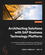
SAP BW Bridge for SAP DWC

In TechEd 2021, SAP introduced SAP BW Bridge for SAP DWC, which allows customers to leverage DWC to support existing investments in their on-premise SAP BW systems and skills in ABAP. The target scenarios for SAP BW Bridge include, but are not limited to, the following:

• Converting SAP BW (BW7.3 and upward) to the cloud while retaining existing data and data flows and leveraging SAC as the consumption layer
• Hybrid scenarios for combining SAP BW4/HANA data and DWC data first, before gradually transitioning the SAP BW4/HANA data flow to DWC

Technically, SAP BW Bridge provides the capabilities for ABAP-based data extraction up to the CompositeProvider level and offers SAP BW4/HANA-like environments in the cloud. However, SAP BW Bridge doesn’t include the OLAP engine and query execution, and add-ons such as the planning engine. Instead, it’s recommended that customers use SAC for planning. Strategically, SAP will continue to invest and evolve SAP DWC so that it becomes the foundation for planning use cases in the future.

In terms of the data sources, it is primarily intended for Operational Data Provisioning (ODP)-based source systems such as ODP-BW, ODP-HANA, ODP-SAP (for SAP S/4HANA), ODP-CDS, and ODP-SLT.

In SAP BW Bridge, customers can use the web-based SAP BW Bridge Cockpit, Eclipse-based BW modeling tools, and ABAP development tools for administration, modeling, and development tasks; the overall experience is very similar to SAP BW4/HANA. At the time of writing, users are still required to work on both BW and DWC environments with these different tools. These tools will be merged to provide a consistent user experience in the cloud in the future.

To enable SAP BW Bridge, a dedicated Space for SAP BW Bridge must be provisioned in the DWC tenant. This Space has a specific type that is different from any other Space. This generated DWC Space contains the connection to an SAP HANA Cloud Smart Data Access (SDA) endpoint and an HTTP-based ABAP endpoint, which can be used to connect the SAP BW Bridge environment with the DWC tenant and the external scheme of the HANA Cloud database underneath SAP BW Bridge, for moving data between the systems. This connection is generated by the provisioning process automatically and cannot be changed by a user. No additional connection can be created in this dedicated Space as it is restricted to SAP BW Bridge only.

Once connected, the tables of SAP BW Bridge can be exposed in the SAP BW Bridge Space in DWC as remote tables. The main purpose of this Space is to import the objects from SAP BW Bridge as remote tables and share them with other Spaces using the cross-space sharing mechanism, which can be used for data modeling. Users cannot create new tables, views, or data flows in this generated space.

During the import, objects in SAP BW Bridge are organized by InfoAreas and underneath data tables of InfoObjects; here, DataStore Objects can be imported into the SAP BW Bridge Space. Within standard DWC Spaces, the shared remote tables can be accessed, combined, and enriched using standard DWC functionalities. Remote table monitoring and remote query monitoring are supported via the Data Integration Monitor.

Finally, SAP BW customers can choose to convert on-premise BW contents using conversion tools, starting from SAP BW7.4, and will support SAP BW7.5 and SAP BW4/HANA in the future. Please check the SAP Roadmap Explorer for the future roadmap of DWC at https://roadmaps.sap.com/board?PRODUCT=73555000100800002141&range=CURRENT-LAST#Q4%202021:

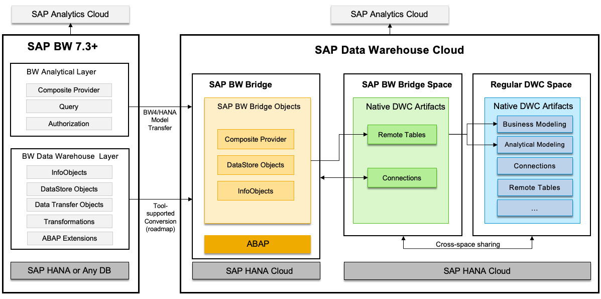
Figure 13.1 – SAP BW Bridge to SAP DWC

Well, we have covered quite a lot, and it might seem quite complicated, but Figure 13.1 gives a good visual recap of what we just discussed.

Data Integration Monitor

While there are multiple ways to integrate data with DWC, how do you monitor and manage the connections and data replications from the source systems? This is what the Data Integration Monitor can help with.

It works like a dashboard and allows you to drill down into the details of a Space. The following capabilities are supported in the Data Integration Monitor:

• Remote Table Monitor to monitor remote tables deployed in the Space, configure data replication options, and refresh the frequency
• View Persistency Monitor to set up persisted views for graphical or SQL views to improve performance as data is replicated and stored locally
• Data Flow Monitor to view and monitor the execution of the flow of the data from source to target and the data transformations in between
• Remote Query Monitor to monitor and analyze the remote query statements and how the communications between the underlying HANA database of the DWC tenant and the remote source systems work

Depending on the use cases, you can decide to access remote data directly or replicate the data to local storage. Both snapshot-based replication (can be scheduled) and real-time replication based on change data capturing are supported. Instead of remote tables, you can also pre-compute the modeled views and configure the data replication for them. Not all the data sources support the real-time replication approach or have delta enabled.

Data Marketplace

So far, we have discussed the various data integration options with DWC for SAP and non-SAP systems, but how about data from other sources or the ecosystem? For that, SAP introduced the Data Marketplace for SAP DWC as its enterprise-grade data sharing and monetization platform.

Within the DWC tenant, you can access or purchase external data from other data providers and combine it with other internal and external data for reporting and analytics use cases. It provides self-service capabilities to avoid the need for long-lasting IT projects for data integration and simplifies how to choose data vendors based on the marketplace catalogs.

Any DWC customer can become a data provider to share and monetize their data assets with other companies, with a strong toolset to create, publish, license, and deliver their data products in an enterprise-grade fashion. This enables SAP customers to benefit from the growing ecosystems of data across various industries and business processes.

Data modeling

Data modeling is a way to define the structure and semantics of data to gain insights from the data based on business requirements. For that, SAP DWC provides two different modeling layers that allow customers to leverage the benefits of business and technical data modeling:

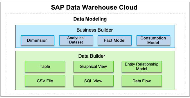
Figure 13.2 – Data Builder and Business Builder in data modeling

The data layer is for technical users, typically data engineers, who can use it to create models in a technical approach. In comparison, the business layer is where the business users can work independently from the technical users in a more business-centric way. With the data layer and business layers, technical users and business users can work together based on the same underlying data. Figure 13.2 depicts the two modeling layers in DWC.

Facts, measures, and dimensions

In data modeling and analytics scenarios, we often speak about the concepts of facts, measures, and dimensions. So, let’s understand them. A fact usually indicates an occurrence or a transaction, such as the sales of a product. A fact can be composed of multiple measures, and most of these measures are quantitative, such as the price of a product or the number of units sold. Dimensions are attributes that have master data, such as a product that provides the context to understand and index the measures. Part of the data modeling approach is applying calculations and aggregations to the quantitative measures and linking them with the dimensions for analytical purposes.

In DWC, there are different types of measures, depending on the type of model:

• Aggregation measures are the default type and aggregate data (sum, average, count, max, and min).
• A derived measure refers to another measure. Here, you can define restrictions on available attributes.
• Calculated measures combine other measures with elementary arithmetic operations (addition, subtraction, multiplication, and division).
• There are also count distinct measures to count the unique occurrence of attributes and fixed value measures for comparisons or to apply further calculations.

Data Builder

Data Builder is where the technical users will do data modeling in DWC, such as creating connections to data sources, preparing, and transforming data, as well as defining the entities and their relationships in an Entity Relationship Diagram (ERD). DWC provides tools for all of these, from uploading a CSV file to data flows to creating graphical views and SQL views.

Entity-relationship models

An entity-relationship (E/R) model is a representation of the relationships of your data entities (tables and views). An E/R model doesn’t contain any data but defines how you organize it logically.

It is quite straightforward to create an E/R model: we drag and drop the data entities and join them together in Data Builder. The created E/R models are available in the Space and other users can reuse them to create views.

Data flows

One of the benefits of data modeling in DWC is that you can use a data flow to create the ETL steps in an easy-to-use way graphically. It allows you to combine both structured and semi-structured data from SAP and non-SAP systems, generic OData APIs, or just files. Different operators support data transformations, such as join, union, projection, or Python operators, which allow you to implement business logic in a script that can be embedded directly in the model. For example, you can apply sentiment analysis in Python using the pandas and NumPy libraries, and then use the result in the model and combine it with other attributes.

Once a data flow has been created and deployed, its execution can be monitored in the Data Integration Monitor. In addition, it can be scheduled to run at regular intervals to keep data updated. Once the execution is completed, the transformed data can be leveraged to create views or for business modeling in Business Builder.

Graphical view and SQL view

In DWC, you can use a graphical interface or write SQL code to create a view. With the graphical view, you can simply drag and drop tables or other views from sources, join them, transform them, and specify measures in the output structure. If the relationship between entities has been defined in an E/R model, they will be joined automatically. If you are comfortable with SQLScript, you can always write the code to create views. A view will be saved in the repository of the Space first and runtime objects will be generated when it is deployed.

Adding business information to views

When creating the views, it is a good practice to add the business information, so it is easier for others to make sense of the data. This enables the business users to perform business modeling in Business Builder, which we will discuss next. We call the business information the semantic layer.

The semantic layer is the information that’s provided in business language to help others understand the data better; for example, adding a new business user-friendly view name or column name. Here is a list of the semantic usage types that can be configured for the tables and views:

• Relational dataset: The default type contains columns with no specific purpose for analytics.
• Dimension: Contains attributes with master data such as a product.
• Analytical dataset: The primary type for analytics; it contains one or more measures and attributes.
• Text: Enables multi-language support for master data. A Text view must be associated with a Dimension view.

You can also define the appropriate semantic type for each column that identifies that a column contains a quantity, a date, and geospatial or other types of information. This can be very useful in data analysis. You can only add semantic types to a column when the view or table it belongs to has the semantic usage set to Dimension or Analytical Dataset. While both views and tables can have semantic usage types, only views can be consumed in SAC or other BI tools. A view will only be available in SAC when it is exposed for consumption and has its semantic usage set to Analytical Dataset with at least one measure.

The facts, measures, and dimensions modeled in the data layer will be visible to the business users, who can use Business Builder to add even more business information to the models.

Business Builder

Business Builder helps model the data in business terms and makes business users more independent from IT. Once data is made available by IT (for example, by creating connections), business users can create data models and collaborate with technical users or other business users based on a semantic view of the data. One of the advantages of DWC is that you can bring together the different parts of the organization with different skills to collaborate and create data models to address concrete business questions.

Using the tables and views from the data layer as the sources, business users can create the business entities in Business Builder. A business entity represents the business objects such as products or sales of products. Dimensions and Analytical Datasets are such business entities. Dimensions only contain the attributes that represent master data. An Analytical Dataset is a fact table that includes both the facts and attributes associated with foreign keys. While the associations can be predefined in the data layer and business users can focus more on the consumption models, business entities are independent of the data layer (including versioning) to allow business users to control and prepare their use cases. You can always enrich business entities with additional calculations.

A fact model groups the analytical datasets and dimensions together and is used to model complex scenarios that need to combine multiple facts and dimensions. Fact models can be nested and thus can be embedded and reused by other users in other models. Consumption models combine the business entities and fact models to create the outputs exposed for consumption, such as in SAC. A consumption model includes one or more perspectives, which is the final consumption unit containing the measures and attributes that can be visualized and analyzed by the analytics clients.

Finally, you will need to restrict access to part of the data in a business context; for example, managers can only access information of employees in their teams. This can be achieved by creating and assigning an authorization scenario. An authorization scenario helps filter data based on some criteria based on data access control, which defines and enforces the filtering by the criteria. You cannot create an authorization scenario on a consumption model, but you can reuse the authorization scenarios that have been assigned to the relevant business entities.

Creating a hierarchy

You may need to organize your data with a proper hierarchical structure. This can be very helpful in many business scenarios. Two types of hierarchies are supported in DWC: parent-child hierarchies and level-based hierarchies. Hierarchies are modeled in Dimensions.

A common example of a parent-child hierarchy is to represent organizational structures, such as HR reporting lines. In this case, members in the hierarchy have the same attributes and it contains a parent attribute to describe the self-joining relationship. For example, immediate managers will be the parents of the employees, even though managers themselves are also employees. The limitation of a parent-child hierarchy is that each node must have a single parent, and data must be normalized to a tree-like structure, which can be very difficult in complex scenarios, such as a matrix organizational structure. Other constraints include that only one hierarchy is allowed in a Dimension, and the attributes that are used for parent keys cannot be composite keys.

A level-based hierarchy is used when your data contains one or multiple levels of aggregation. It is not recursive, and each hierarchy has a fixed number of levels in a fixed order. Typical examples of level-based hierarchies are time-based hierarchies (Year, Quarter, Month, Week, and Date) and location-based hierarchies (Region, Country, State, and City). You can navigate the hierarchy to drill up and drill down in analytics; each level contains the aggregated values for the levels below it.

Data consumption

The consumption layer of DWC is created by integrating with SAC. SAC connects with DWC through remote connections to build stories on top of analytical datasets and perspectives exposed for consumption. You can also connect with third-party BI tools with your Space data to build visualizations.

Working with SAC

To build stories and analytics applications with SAC, you can expose your DWC Space data through the live connections between SAC and DWC tenants.

Before release 2021.03, DWC offered an embedded version of SAC where DWC and SAC were run in the same tenant, and stories that were created in SAC were saved directly in the DWC Space. This is called Space-aware connectivity. There are limitations of embedded SAC; for example, it is limited to five user licenses. SAP recommends only using the embedded version for testing purposes. For tenants provisioned after 2021.03, customers will need to have two separate tenants – one for DWC and another for SAC.

Technically, a SAC tenant can connect to multiple DWC tenants as data sources and combine them with additional data to create stories. Any DWC tenant can be connected to any SAC tenant through a live connection. To consume data and models from DWC, it is important to expose them for consumption, which can be enabled in either Data Builder or Business Builder for the respective objects.

DWC and SAC share the same authentication mechanism and Identity Provider (IdP) settings. You can also link the DWC tenant with the SAC tenant through Tenant Links to enable the product switch to easily navigate between them on the UI.

There are certain product limitations of the live connections. Please check SAP Note 2032606 for more details at https://launchpad.support.sap.com/#/notes/2832606.

Working with third-party BI tools

To connect a DWC tenant with third-party BI Tools such as tableau or Microsoft Power BI, an ODBC driver needs to be installed. The IP address of the tool needs to be added to the allow list in the DWC configuration. Since it is a SQL-based connection, a database user who has access to the Space schema needs to be created and objects for consumption in a third-party tool must be exposed in DWC. Once connected, you can use the DWC objects to create visualizations with your existing BI tools.

Audit logging

Audit logs help you understand who did what, where, and when. It is important for your security, auditing, and compliance teams to monitor possible vulnerabilities or data misuse. In DWC, you can set up audit logging for both change operations and read accesses, which can be configured separately. It can be enabled at the Space level and the retention time can be configured from 7 days to a maximum of 10,000 days. The default retention time is 30 days. Based on your business requirements, you can determine your retention policy. Please be aware that audit logs also consume the storage capacity of your DWC tenant.

For individual database schemas such as Open SQL schemas created for database users, the audit logs need to be enabled separately. Please note that statements executed in SAP HANA Cloud, data lake through the wrapper procedures are not audited currently.

To view the audit logs, SAP recommends creating a dedicated Space for audit logs so that only users with access to this Space can see the logs. These logs are saved in the AUDIT_LOG view of the DWC_AUDIT_READER schema and the ANALYSIS_AUDIT_LOG view for database analysis users separately.

This wraps up our introduction to SAP DWC, where we focused on data integration and data modeling. Next, we will discuss SAC as the consumption layer of DWC and how it can be used for advanced analytics scenarios.

SAP Analytics Cloud (SAC)

SAC is a SaaS offering for analytics that combines capabilities such as BI, enterprise planning, and predictive analytics into one product. SAC is the analytics layer and provides a consistent experience for all SAP applications through embedded analytics and enterprise analytics use cases.

Connectivity

SAC can access data from cloud data sources or on-premise systems by providing two types of connectivity, online live connections, and batch-based data acquisitions. Live connections allow you to build stories and perform analytics with live data without any data replication. In data acquisitions, data is imported into SAC and its underlying HANA database first. You may be wondering what the right approach is for your specific use cases. Please refer to Table 13.1, which shows the criteria you must consider when choosing the right approach:

Criteria	Live Connection	Data Acquisition
Functional	Performance and product limitations may apply. No planning support on the live connection. Available for HANA, DWC, BW, BOE Universe, and S/4HANA.	Support analytics, planning, and predictive scenarios. Available for SAP cloud applications and third-party data sources.
Data Storage	Data stays in the source system and connects to SAC in real time.	SAC stores the model and data locally in its underlying HANA database.
Data Security and Privacy	Managed on the source system. This is preferred when full control of data is required, and data cannot leave the source system.	Security is added to the models within SAC, and data is fully encrypted and secured.
Data Volume	No theoretical limitations as the data is processed in the backend. However, it needs to apply adequate filtering and aggregation to limit the volume returning to the web browser.	Limitation in file sizes (< 200 MB for Excel files and < 2 GB for CSV files), row and column counts (< 2 B rows, < 100 columns in models, < 1,000 columns in datasets), and cell sizes.

Table 13.1 – Live connections and data acquisition

Understanding live connections

Unlike the live connection we discussed in HANA Cloud and DWC through the data federation at the HANA database level, the live connections between SAC and the data source systems are mainly browser-based. In this case, SAC only stores the metadata (for example, measures, column names, and filter values) for building the stories and queries. The browser, in turn, sends queries through a live connection to the source HANA database that executes the queries and returns the results to SAC to render the charts. None of the actual data or query results will be stored in SAC. All communication between the browser and SAC is encrypted, and all metadata persisted in SAC is fully encrypted.

In the live connection scenario, the browser must access SAC for metadata and the data source at the same time. The same-origin policy is a critical security mechanism that restricts how a resource in an origin can interact with resources in another origin, to reduce possible attach vectors to isolate and prevent potentially malicious documents. SAC supports a direct live connection by leveraging Cross-Origin Resource Sharing (CORS) as a mechanism (use additional HTTP headers) to connect with data sources such as HANA on-premise, SAP BW, and SAP S/4HANA. In these cases, CORS must be enabled at the data sources and the browser must accept third-party cookies and disable the popup blocker.

The most secure way to connect to an on-premise data source is through the SAP Cloud Connector by creating a secure tunnel between the data source and SAP BTP where SAC is hosted. It acts as a reverse proxy and the communications are always initiated by the SAP Cloud Connector, so there is no need to open any port in the firewall to the on-premise systems. The trust to SAP Cloud Connector is configured in SAC to a specific SAC subaccount in SAP BTP. All communications across the tunnel are secured based on Transport Layer Security (TLS) and can be monitored and audited within SAP Cloud Connector. You learned more about SAP Cloud Connector in Chapter 4, Security and Connectivity.

For cloud data sources such as SAP HANA Cloud and SAP DWC, there are dedicated connection types. For example, the SAP HANA Cloud connection type is highly recommended for live connections to HANA Cloud databases. For previous offerings of HANA in the cloud such as HANA 2.0 hosted in BTP, you can create a live connection using the SAP HANA Analytics Adaptor for Cloud Foundry. In embedded analytics scenarios where SAC is embedded in a cloud application such as SAP SuccessFactors Core HXM, the SAC OEM integration service is leveraged. The key responsibility of these adapters or integration services is to act as the proxy to execute queries in the data source system based on the SAP Information Access Service (InA) protocol, which defines queries using rich or complex semantics to perform multidimensional analytics, planning, and search data in HANA.

To provide a better user experience, single sign-on (SSO) should be enabled between SAC and the data source systems by using the SAML 2.0 protocol and have a common authentication based on the same IdP. For SAP applications, SAP Identity Authentication Service (IAS) is the default IdP, though it can also act as the proxy to delegate the authentication to another IdP of the customer’s choosing.

Figure 13.3 depicts the live connection options:

Figure 13.3 – SAC live connections overview

Important Information

To learn more about the limitations of live data connections, please check https://help.sap.com/viewer/00f68c2e08b941f081002fd3691d86a7/release/en-US/6ac0d03d53f3454f83d41c6f51c2fc31.html.

Understanding data acquisition

If combining multiple data sources and blending data through live connections is not sufficient, for example, due to large data volume and high-performance requirements, then you should consider using the data acquisition approach to replicate data into SAC. Here, data is copied and stored in the underlying HANA database of SAC.

While the live connections mainly work for HANA-based systems and SAP Universe or Web Intelligence, you can replicate data from many more cloud and on-premise data sources. Most SAP cloud applications such as SAP SuccessFactors, SAP Concur, SAP Fieldglass, and Qualtrics provide data integrations with SAC through a common integration interface based on the OData protocol. SAC also supports integrations with Google Drive, Google Big Query, Salesforce, Dow Jones, and others through dedicated connectors. Additional non-SAP applications are supported through SAP Integration Suite Open Connectors.

For connectivity with on-premise data sources, such as live connections, SAP Cloud Connector is required to establish the secure tunnel and act as the reverse proxy. To connect with SAP BW, SAP Business Planning and Consolidation for Microsoft (BPC MS), SAP BusinessObjects Business Intelligence platform universe (UNX), and SAP Enterprise Resource Planning (ERP), a SAC agent must be installed and configured. It is recommended to install an SAC agent and SAP Cloud Connector on the same server. Figure 13.4 summarizes the options for data acquisition:

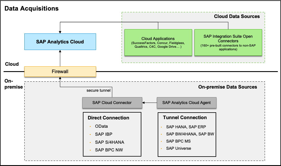
Figure 13.4 – SAC data acquisition overview

Important information

To learn more about the limitations of data acquisition, please refer to the official document at https://help.sap.com/viewer/00f68c2e08b941f081002fd3691d86a7/release/en-US/5f61b6509a5e4d499e8cb9685f32db73.html?q=sizing#loio5f61b6509a5e4d499e8cb9685f32db73__section_tuning.

Data preparation

Before creating a story, you will need to prepare data. In SAC, preparing the acquired data can be done using either a dataset or a model. A dataset is not a new concept but has been used in Smart Predict behind the scenes before. The new data preparation experience called Smart Wrangling uses datasets directly within the scope of a story, instead of a model.

One of the advantages of using datasets is the reactivity to changes in a more efficient way. This is because the data structures of datasets and models are different. Datasets store data in a single table with a semantic structure defined by the metadata, so it is considered a lightweight object. In comparison, models store data in a star schema with measures and multiple dimensions. Imagine that you need to change the data type of an attribute from a dimension to a measure; SAC just needs to update the metadata of a dataset instead of updating the fact table and dimension tables such as when using a model, which is more time-consuming. This allows you to quickly toggle back and forth between story creation and data wrangling when building a story, so there is no need to prepare data perfectly upfront. SAC users can greatly benefit from this agility and integrated workflow.

Models are preferred if the structure of data has already been defined before a story is created and it supports fine-grained data management. This is better for data governance and planning use cases. Table 13.2 summarizes the differences between datasets and models:

	Dataset	Model
Use Cases	Ad hoc data, agile story building with data wrangling, predictive scenarios with Smart Predict	Governed data and the preferred format for live data, planning, and time series forecast scenarios
Data Management	Stored as a table with separate metadata within a story or as a standalone dataset, limited data management	Stored as a star schema with measures and dimensions, only exists outside a story, fine-grained data management
Data Access	No row-level security and can access the dataset as a whole	Row-level security, supports data access control per the dimension value

Table 13.2 – Datasets versus models

There are various tools you can use to edit the data in a dataset to clean, enrich, and transform the data into the desired structure. For example, you can change measures and dimensions, resolve data quality issues such as setting default values for missing data, add geo-enriched data with coordinates or areas such as countries and regions, define level-based hierarchies, update aggregation types for measures, and more. One of the cool features is the Custom Expression Editor, which allows you to implement complex transformations such as calculating a new column based on other columns. The custom logic is implemented in scripts with the support of operators for different data types.

From a business scenario perspective, there are two types of models – analytic models and planning models. Planning models are preconfigured to support the planning process, such as forecasting, and come with some default configurations and features such as categories for budget, plans and forecast, a date dimension, and additional auditing and security features. Analytics models are more flexible for general-purpose data analysis. Analytics models work with both live data and acquired data while planning models only work with acquired data.

In addition, depending on how the measures are structured, there are two types of models – the classic account model and the new model. Launched in the Q2/2021 QRC release of SAC, the new model is a significant change in how models are structured around the measures. It is based on the learnings from the Account model, which originated from the planning scenario. The new model enables greater flexibility and adds benefits in both analytics and planning scenarios in multiple areas:

• A flexible model structure that supports model configuration with measures, an account dimension, or both. This flexibility allows more accurate aggregation over measures and explicit data types (decimals and integers).
• Improved calculations on measures and numeric dimension properties. Calculated measures in models can be reused in stories and analytics applications.
• Better data integration with the measure-based model aligns better with other SAP systems such as S/4HANA and SAP BW. This means less transformation is required to import data from source systems into the target models.
• Improved data wrangling with a custom expression script, which acts like a dataset, is now available in the new models.
• Multiple base currencies and conversion measures in the models support planning on multiple currencies and allow you to see the results across dependent currencies.

The new model type offers more flexibility, and it is possible to convert from the classical account model into the new model with measures. To convert, the dependencies must be resolved (for example, if a model is used by stories), and currency conversion should be turned off. After the conversion, the data import/export jobs need to be updated so that they fit into the new target model. At the time of writing, models created from a CSV file or Excel file are based on the classic account model. Figure 13.5 illustrates how to convert from a classic account model to a new model:

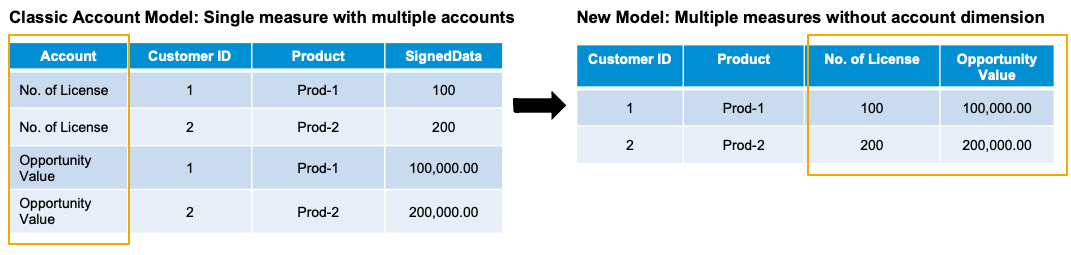
Figure 13.5 – Classic account model and the new model

While SAC provides the necessary data modeling capabilities, more features are available in SAP DWC, as discussed earlier in this chapter. In that case, most data modeling is performed in DWC and exposed for SAC to consume via a live connection between SAC and DWC.

Creating stories with Story Designer

Data visualization is a great tool for telling the stories behind data. It helps the consumers interpret and understand data at a faster pace and makes it easier to recognize patterns and identify exceptions. In SAC, a Story is a presentation-style document that uses visualizations to describe and analyze data.

There are many ways to visualize data, and choosing the right visualization can have a big impact on how easily the users will be able to consume the information. So, before starting with visualization, it is important to understand your audiences – for example, what story you want to tell, what questions should be answered, and what insights the data will give.

While the design aspect of a story can depend on many aspects and it is hard to compare which design or style is better, there is some general advice from SAP and the SAC community to consider:

• Start from the big picture to design the high-level summary pages first and then drill down into detailed pages for more insights.
• The main information should come first, without the need to scroll down the page. Group the related information to make it easier to compare and analyze.
• Use colors when appropriate, don’t make a dashboard too colorful, and use the same color theme throughout the entire story.
• Use the best-fit charts for the data. For example, a pie chart is not recommended when there are too many values to present.
• Apply a standard checklist for all visualizations to check text alignment, chart sorting, ranking, font type and size, and more.
• Follow corporate brand design guidelines whenever applicable – for example, if the corporate has specified the color schemes, background colors, logo size, and placement.

It is not easy to keep all stories consistent in terms of colors, fonts, and corporate standards. This is where story templates can be considered. SAP Analytics templates, which are created by administrators, are the global templates saved in the default Sample folder, which is visible to all users who can create stories from a template. A story template defines not only the colors and formatting but also the page layout, background, default color, font and border, default table setting, input controls styling, and more.

Story pages

A story page can be a blank canvas, a responsible page, or a grid for different kinds of use cases. Responsive pages allow you to create lanes to section the page into groups; widgets within a lane will stay together when the page is resized. You can run the device preview to see what the page will look like in different screen sizes and device types.

A canvas page is a flexible space where you can add charts, tables, geo maps, or other visualizations and apply styling either to individual objects or groups. A canvas page can be used to create a reporting layout by adding a header and footer. Grid pages are best for working with tabular data, just like Excel sheets. They are especially useful when working with numbers and formulas.

Linked analysis and linked models

A Story often contains multiple charts or tables. Linked analytics enables the interactions between the different widgets, for example, by applying a filter or drilling through hierarchical data in one chart and seeing the update in linked charts. Linked analytics must be based on the same underlying model or across different models with linked dimensions.

When performing cross-model linked analysis, you must set up the link between models by defining the common dimensions. Once this link has been established, applying a filter to one model can influence the widgets based on the linked model. Filtering across models works for linked dimensions directly and other unlinked dimensions indirectly. For indirectly filtering on unlinked dimensions, even though it can achieve a similar filtering experience, it is usually performance intensive as technically, it will apply the filter on a model first and pass all the filtered values of the linked dimension to the model that doesn’t have the dimension that the filter is based on. To optimize performance, link the dimensions directly whenever possible or link as few dimensions as possible if the dimension to be filtered cannot be linked. You can specify the Linked item set to apply the filtering and then drill through hierarchal data for all the charts in the same story, on the same page, or only for selective charts.

While linked analysis enables filtering across models, data blending is the process of adding a linked model to the primary model. This allows you to combine data from multiple models in a chart or table. For example, you can combine data from a BW live connection with imported data from an Excel spreadsheet. Both linked analysis and linked models start by defining the common dimensions to link the models. Once linked, the dimensions and measures from both models can be used in the visualizations.

In SAC, there are two types of data blending – browser-based blending and Smart Data Integration (SDI)-based blending. Browser-based blending doesn’t require you to install anything. At the time of writing, you can blend data from a BW live connection with imported data, a HANA live connection with imported data, and a S/4HANA live connection with imported data. It is easier to start with browser-based blending, but there are limits in terms of data volume. For example, it supports up to 2 MB in dataset size for HANA live connection scenarios. SDI-based blending is recommended for larger datasets and supports more data sources. For this, you must install and configure the Data Provisioning Agent.

When blending the models, links between models only occur within the story; no new model is created. There are other restrictions in linked models – for example, geo maps are not supported, and blending across multiple live connections is not supported.

Digital Boardroom

Digital Boardroom, which is built on SAC, is a presentation tool that combines stories with agenda items, to enable decision-makers to make collaborative and data-driven decisions based on real-time data. It integrates multiple data sources to produce a single source of truth and enables the drill-down analysis from aggregated insights to the line items. Besides this, decision-makers can adjust drivers and run simulations to see the impacts of a decision and predict the outcomes. Digital Boardroom is an add-on to SAC’s existing use licenses.

Creating analytics applications with Analytics Designer

Business users create stories in a self-service workflow using the various widgets and configurations with guided steps in the story design-time environment. However, the amount of customization is limited in stories.

In comparison, an analytics application typically contains some custom logic and requires more flexibility to present and interact with data, ranging from simple dashboards to highly customized and complex applications. For example, you can dynamically switch between different chart types at runtime.

Unlike stories designed for business users, analytics applications have more freedom to change the default behavior and usually require developer skills to implement custom logic with scripting. Stories and analytics applications are two different artifacts in SAC with corresponding design-time environments. However, stories and analytics applications are similar from a consumption perspective, with a similar look and feel, and share the same widgets and functionalities.

Analytics Designer is the dedicated low-code development environment for creating interactive analytics applications in SAC, which includes the capabilities to define data models, create and configure widgets, build UIs and layouts, and implement custom logic with the help of scripting through JavaScript-based APIs (Analytics Designer API Reference Guide at https://help.sap.com/doc/958d4c11261f42e992e8d01a4c0dde25/release/en-US/index.html).

An analytics application can be embedded with the support of bi-directional communication, which passes parameters through APIs so that they can interact between the embedding application and the embedded analytics application. This is extremely useful for insight-to-action-like scenarios, such as finding valuable insights from a dashboard to trigger actions through an OData call in a transactional system and seeing the outcome reflected in the same dashboard in real time. This helps achieve close-the-loop scenarios.

Analytics Designer completes SAC in addition to its BI, planning, and predictive capabilities and brings them together, and enables agile development by leveraging existing functionality and connectivity for more interactive use cases. Since it is built on top of SAC, you can create integrated planning applications, and use all the smart features such as Smart Insights and Smart Discovery in the analytics applications. R scripts can be involved to create a lot of different types of visualizations using libraries such as ggplot2. Furthermore, custom widgets can be created with a provided SDK; they can be set in the widget palette and work like the predefined widget. Creating a custom widget requires two files. First, there is a JSON file for metadata, which defines the ID, properties, events, and methods and specifies the location of the web component. The metadata file must be uploaded to the SAC tenant. The actual web component can be deployed remotely, and it is written in JavaScript. It contains the implementation as an HTML element.

To summarize, Analytics Designer extends the use cases beyond transitional analytics scenarios and supports sophisticated applications while leveraging the same design, concepts, and capabilities of SAC. There are many more things you can achieve with Analytics Designer. The developer handbook is one of the best resources for exploring and learning more about Analytics Designer: https://d.dam.sap.com/a/3Y16uka/SAPAnalyticsCloud_AnalyticsDesigner_DeveloperHandbook.pdf.

Content Network

Business content in SAC includes models, stories, and SAP Digital Boardroom presentations and they are providing the actual values for businesses to accelerate analytics content creation and data-driven workflows. The Content Network is where the business content is stored, managed, shared, and consumed. Content packages are organized by industries or LoBs. There are content packages from both SAP and third-party partners. Some third-party content is paid content; most of them also provide a trial option and customers can purchase the full version later through the SAP Store, which is the marketplace for SAP solutions or extensions from the partner ecosystem of SAP.

After importing the content package into your own SAC tenant, you will need to connect the content with your data. The business contents in the Content Network usually have two ways to connect with data – data acquisition or live connection. The contents that come with data acquisition are usually ready to run immediately with the sample data included that’s facilitated by the models without additional effort. However, it is not recommended for productive use, which is required to import data from the actual data source or establish a live connection with the source system. The sample data should be cleared before you load the actual data. For content based on live data connectivity, no sample data is provided, so you will need to establish a connection with the data source to view the visualizations.

While there are many advantages to using the Content Network to import, export, and share content packages, it is always recommended to import and copy the content to a different folder to prevent any accidental loss of modifications and customizations during a re-import or a version update from the Content Network when the Overwrite objects and data option is selected. Content in Content Networks is forward-compatible, but there is no guarantee of backward compatibility.

For the latest information on published content in the Content Network and how to use it, please check out the Content Network Release Information Guide at https://help.sap.com/viewer/21868089d6ae4c5ab55f599c691726be/release/en-US/975ca591bc45435b8ebe89a210757466.html and the Content Package User Guide at https://help.sap.com/viewer/42093f14b43c485fbe3adbbe81eff6c8/release/en-US.

Embedded analytics

Embedded analytics allows you to analyze and visualize data directly in the source system without the need for complicated data preparational steps. The embedded SAC offers predefined dashboards, personalized data access, integrated role and screen variants of S4/HANA, and an intuitive ad hoc reporting capability for business users to gain insights from data. Besides this, with SAC as the analytics layer, it provides a consistent experience across SAP applications. At the time of writing, embedded analytics is available in S/4HANA Cloud, SuccessFactors, and Fieldglass solutions.

So, how does embedded analytics work technically? Let’s take S/4HANA embedded analytics as an example. For each S4/HANA Cloud tenant, an SAC tenant is provisioned with it. SAC accesses the S/4HANA system through live access to ABAP CDS Views via underlying persistent data models and uses the transient queries generated from the CDS views. The relevant features, such as tenant provisioning, connectivity, and content life cycle management, are exposed through SAC APIs that are involved and fully managed by the embedding application, such as S/4HANA. The UI of SAC is embedded as iFrames in S/4HANA’s Fiori-based UI, whereas SAC stories are integrated by a wrapper application that supports screen-variant savings, personalization, and intent-based navigations between analytical and transactional applications. Custom content is supported as you can create custom ABAP CDS Views and build stories and dashboards on top. Custom content can be exported and imported through Extensibility Inventory, which leverages Analytics Content Network (ACN) to move contents between tenants. The life cycle of analytical contents such as data models, KPI definitions, and preconfigured dashboards are integrated into the application life cycle management of the embedding application. Embedded analytics doesn’t require an additional license as it is already included as part of the applicable licenses.

Figure 13.6 provides a high-level overview of the integration architecture of the embedded analytics scenario. The following are the detailed steps for setting it up:

1. The SAC OEM tenant is provisioned together with the embedding application.
2. SAC and the embedding application must have a common authentication based on a shared IdP. SAC users are created via the identity service or SAC User and Team Provisioning API. Users are kept in sync between SAC and the embedding application.
3. Applications deliver predefined content, which is the metadata to describe data models, queries, and other analytical contents. Such contents will be provisioned into the SAC OEM tenant.
4. SAC accesses the application data through the SAC OEM integration service, which uses the live connection to access the underlying HANA database of the embedding application. The integration service provides a metadata adapter, runtime authentication and authorization, multi-tenancy handling, and an InA provider for runtime query metadata and data access.
5. SAC UI is embedded in the application UI through iFrames:

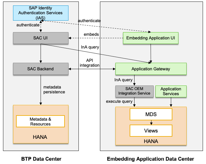
Figure 13.6 – Embedded analytics integration architecture

The integration service uses the Core Schema Notation (CSN) for the semantics of data structure. It supports the ad hoc data modeling tool Query Designer for end users, thus enabling self-service for business users in addition to predefined dashboards.

However, embedded analytics is exclusively bonded to the embedding application, meaning it cannot be used by other applications. If you are interested in business scenarios that will require data from multiple applications, you will need an enterprise SAC tenant. More differences between embedded analytics and enterprise analytics are shown in Table 13.3:

	Embedded Analytics	Enterprise Analytics
Data Sources	Restricted to embedding applications through live connections only	Can connect to various SAP and non-SAP data sources through live connections and data acquisitions; supports data blending from multiple data sources
Prebuilt Analytics Content	Prebuilt dashboard for the embedding application; content delivery by the application can only be done through SAC APIs	Comprehensive content packages from SAP and third parties through the Content Network library
Smart Features	None of the smart features or R-Visualization are available	Supports Search to Insight, Smart Insights, Smart Discovery, Smart Predict, and R-Visualization
Planning	Doesn’t support planning processes	Supports operational, strategic, and financial planning
Insights to Action	Out-of-the-box integration with the embedding application	No out-of-the-box setup
User and Role	Reuse roles from the embedding application	A separate set of roles and authorizations need to be setup
Add-Ons and Custom App Support	No add-on support	Supports multidimensional analysis via Excel-based add-ons, Digital Boardroom, and custom widget design
License	Doesn’t require any separate license	Requires separate SAC licenses

Table 13.3 – Embedded analytics and enterprise analytics scenarios

SAC APIs

SAC provides REST APIs to support the automation of administrative tasks such as user creation. Before using an API, you must create an OAuth client in the SAC tenant. In SAC, the following APIs are available:

• OEM Tenant Management APIs: These allow applications to create and manage SAC tenants and configure them, such as by adding a live connection, an OAuth client, or a trusted IdP. It also provides APIs for getting the quotas for each landscape and retrieving the logs. Multitenancy support for the application is facilitated by the OEM integration service with the support of the Tenant Configuration API when it processes the data and metadata by supplying the tenant ID context.
• Open Story and Application URL APIs: These allow applications to access a story and analytical application directly via a URL, which can be used for embedding SAC in the UI of your application as an iFrame control.
• SAC Tenant APIs: These allow applications to access information of the SAC tenant such as stories and metadata, users, groups, the permissions of SAC artifacts, and the User and Team provisioning System for Cross-Domain Identity Management (SCIM) API for managing users and teams programmatically for tasks such as creating users, assigning users to teams, enabling correct user setting for language, date, time, and number formats, updating SAML mapping for SSO, changing licenses, transporting users and teams between different tenants, and more.
• Content Network APIs: These allow you to manage analytical content through APIs, such as getting the list, details, and permissions of items in the Content Network, creating an import job, and getting the job’s status.
• Analytics Designer APIs: These can be used to create interactive and custom-designed analytical applications as you can write scripts for interactions. For example, you can assign a script to a button’s onClick event when the user selects it within a chart. Scripts are based on JavaScript and are available to almost all controls in SAC.

Most of these APIs have been published on SAP API Business Hub at https://api.sap.com/package/SAPAnalyticsCloud/rest.

Smart features

SAC includes a variety of smart features for leveraging machine learning and natural language processing technology to help you explore data and gain insights from data. These smart features are called augmented analytics in SAC and range from using natural language to search and generate visualizations automatically, to making predictions and recommendations from historical data.

Search to Insight

Search to Insight provides a Google-like interface for querying data using natural language directly from the Story. Users can ask questions and SAC will create the most appropriate visualizations for the questions. For example, you can ask questions about showing the top five sales by region. Follow-up questions are supported in the same business context; for example, you can run subsequent searches by specifying the product types or other dimensions, such as showing the sales by product for the last four quarters. While typing a question, auto-completion is supported for dimension names, dimension values, and measure names. Synonyms can be created for dimension and measure names and used in the query.

The generated charts are interactive, and you can also change the chart types. The charts of Search to Insight can be embedded into a Story directly by simply copying and pasting. This democratizes the story creation process by enabling the user to use natural language to build visualizations.

Search to Insight works with indexed data models either through data acquisition or live connection (limit to 5 million members for indexes based on live data models) and supports data sources such as SAP HANA, SAP S/4HANA, SAP Universe, SAP DWC, and SAP BW. Visualizations based on indexed data are determined by the date access rights of the users. At the time of writing, Search to Insight only supports querying questions in English.

Smart Insights and Smart Discovery

Smart Insights and Smart Discovery are two advanced features in SAC that use ML/AI technologies to help users gain insights from the data. Smart Insights identifies the top contributors of a selected value or variance point, while Smart Discovery identifies the key influencers of a selected measure or dimension.

Smart Insights identifies the top contributors that have the highest contributions to the data points being analyzed – for example, what contributed most to revenue across the regions, such as North America. The generated insights are explained in natural language. We can deep dive into the generated result and investigate it further by running Smart Insights again for the North American region to understand the different sets of top contributors, such as product types, customer segments, and more. It doesn’t only explain what top contributors are but also how they are calculated.

By using Smart Insights in combination with Variances, you can quickly identify the positive and negative influence factors behind the variance, such as those between actual and budget sales.

Smart Insights is a significant time-saver for business users looking for insights into a particular value; otherwise, they may have to investigate the members of each dimension to understand how they will contribute to the result. Smart Insights only works for a single data point or variance. It can be enabled by simply clicking a data point in a chart and using the right-click context menu, and then selecting the light bulb symbol to open the Smart Insights side panel.

In comparison, Smart Discovery works against a data model as an automated data exploration tool to identify key influencers and explore the key differences between the different attributes. It is especially useful for open-ended questions. Users can run the discovery against a measure or a dimension. Here, it will build regression models for measures to predict future outcomes and classification models for dimensions to segregate results into different groups.

During runtime, Smart Discovery will build and test multiple models and determine the best fit model based on accuracy and robustness to generate the results. It does so in the form of intuitive charts and correlations explained in natural language. It helps you discover the key influencing factors and understand the positive or native impacts of each influencer, how they are related to each other, and the results.

Smart Discovery helps users start analysis right away and gradually explore the key influencers in great detail. Besides this, it works nicely with Smart Insights, which provides more insights for a selected value.

Table 13.4 summarizes the differences between Smart Insights and Smart Discovery:

	Smart Insights	Smart Discovery
Features	Identifies the top contributors and various insights for the selected value or variance. They are visualized in the Smart Insights side panel, with different types of charts and dynamic text explanations.	Identifies key influencers for selected dimensions or measures and explores the relationship between different attributes. The results are presented in a generated story that covers key influencers, unexpected values, and simulations.
Use Case	Looks for insights for a particular value, performs deep-dive analysis, and explains surprising elements in data. An example of a use case is as follows: Understand what contributed most to the revenue for a county	Jump starts data exploration, understands what is relevant to a result and the complex relationships and outliners, and performs what-if-like simulations. An example of a use case is as follows: Discover how sales or marketing activities influence the revenue
Data Context	Single data point or variance	A data model with multiple dimensions and measures

Table 13.4 – Smart Insights and Smart Discovery

Smart Predict

Smart Predict is an advanced feature designed for a business analyst to leverage machine learning to answer business questions about future trends and make recommendations. The users are guided through the predictive workflows, and basic knowledge of statistics and machine learning is required. In this section, we will focus on Smart Predict, though SAC for planning includes a variety of features that help generate planning forecasts by analyzing the historical data while leveraging the same techniques. We will cover predictive planning later.

Three types of predictive scenarios can be created:

• Classification ranks the population and predicts the probability that an event will happen. For example, who is likely to buy a product based on buying history data?
• Regression finds the relationship between variables and estimates the value of a measure. For example, how much would a customer spend in my store?
• Time Series Forecasting predicts the values of a time-dependent measure. For example, what are the expected sales by products for the next few weeks?

The quality of data is important when building a predictive model; the training dataset must represent the business domain and the predictive goals. Among the variables, one of them is special – the target variable that you want to predict. For classification, the target variable is a categorical value while the target is a numeric value for a regression model. Variables that are highly correlated to the target variable are called leaker variables and they must be excluded to avoid something having a dominating influence on the results.

During the training process, Smart Predict assigns 75% of the dataset as the estimation dataset to build the predictive model; the remaining 25% is used for the validation dataset to calculate the performance of the model. For the prediction, the dataset must have the same structure as the training dataset. This means it must have the same number of variables and the same variable names and types as the training dataset.

Once the predictive model has been trained and run, you can evaluate the accuracy and robustness of the model by using performance indicators such as Prediction Power and Prediction Confidence, and built-in reports in SAC such as Confusion Matrix. We will discuss these later in this section. The predictive outputs can easily be stored and visualized in SAC stories, as well as used in other models such as a planning model.

Before we discuss each of the predictive scenarios, we’d like to share a little bit more background on how predictive analytics has been evolved in SAC. The model behind the prediction initially came to SAC from SAP’s acquisition of a predictive analytics company called KXEN. KXEN’s predictive models were based on an algorithm named Ridge Regression. Ridge Regression has been found to work well, unlike Ordinary Least Square Regression (OLS), which overfits and tries too hard to fit all data points. However, it does assume the predictions will have a linear relationship with predictors.

SAC Smart Predict is now based on Gradient Boosting, which has made substantial improvements in the model performance. At the core of Gradient Boosting is a data structure called a tree. It uses a collection of trees, with a philosophy to iteratively build weak learners and then combining them will create accurate and robust predictions.

For example, if you take the dataset and fit the first tree first, and the first prediction is more distant from the truth and left with a residual (the difference between the predictions and actual values), then you can build another tree to explain the residual until you reach a point where most of the residuals have been explained or the maximum number of trees has been reached (this is limited to four levels to avoid overfitting and reduce model complexity). For structured datasets, Gradient Boosting has been proven to outperform the previous version of Smart Predict, which is why it has been chosen for the new predictive models in SAC.

Classification

Classification is used to predict the probability that an event will happen. For example, it can help predict scenarios such as which customer is likely to churn or which employee may potentially leave the company. At the time of writing, SAC Smart Predict only supports binary cases in classification.

To rank a population and make a prediction, the quality of the data is important to build a predictive model. A good predictive model finds the right balance between accuracy and robustness, can predict correctly, and avoid overfitting, is robust, and can be trusted to predict new cases. The performance of a classification model is usually measured by two indicators:

• Predictive power measures the accuracy and quality of the model. It is the ratio between correct predictions and total cases, ranging between 0 and 1.
• Prediction confidence measures the robustness of the model and represents that the model can be used to predict new cases reliably. It can be increased by improving the training dataset.

The classification model also explains the influencers and how these variables are contributing to the target. The top ones are summarized on the Influence Contributions page, which allows the user to navigate and understand the relationship between different variables. For example, in the use case of whether a customer is likely to churn, you can analyze how the customer segments, industries, countries, and LoB may impact the results.

Other useful tools include Confusion Matrix and Profit Simulation, which allow you to choose a threshold on the percentage of the population to predict the results. For example, if you select 20% of your customers with a high probability of churn, what is the percentage of that 20% you are likely to keep if you can prioritize your customer success activities to retain these customers? This is very helpful, for example, if you have a limited budget and need to determine and find the balance between costs and outcomes. Figure 13.7 depicts the predictive model performance metrics and top influencers for predicting whether a customer will churn:

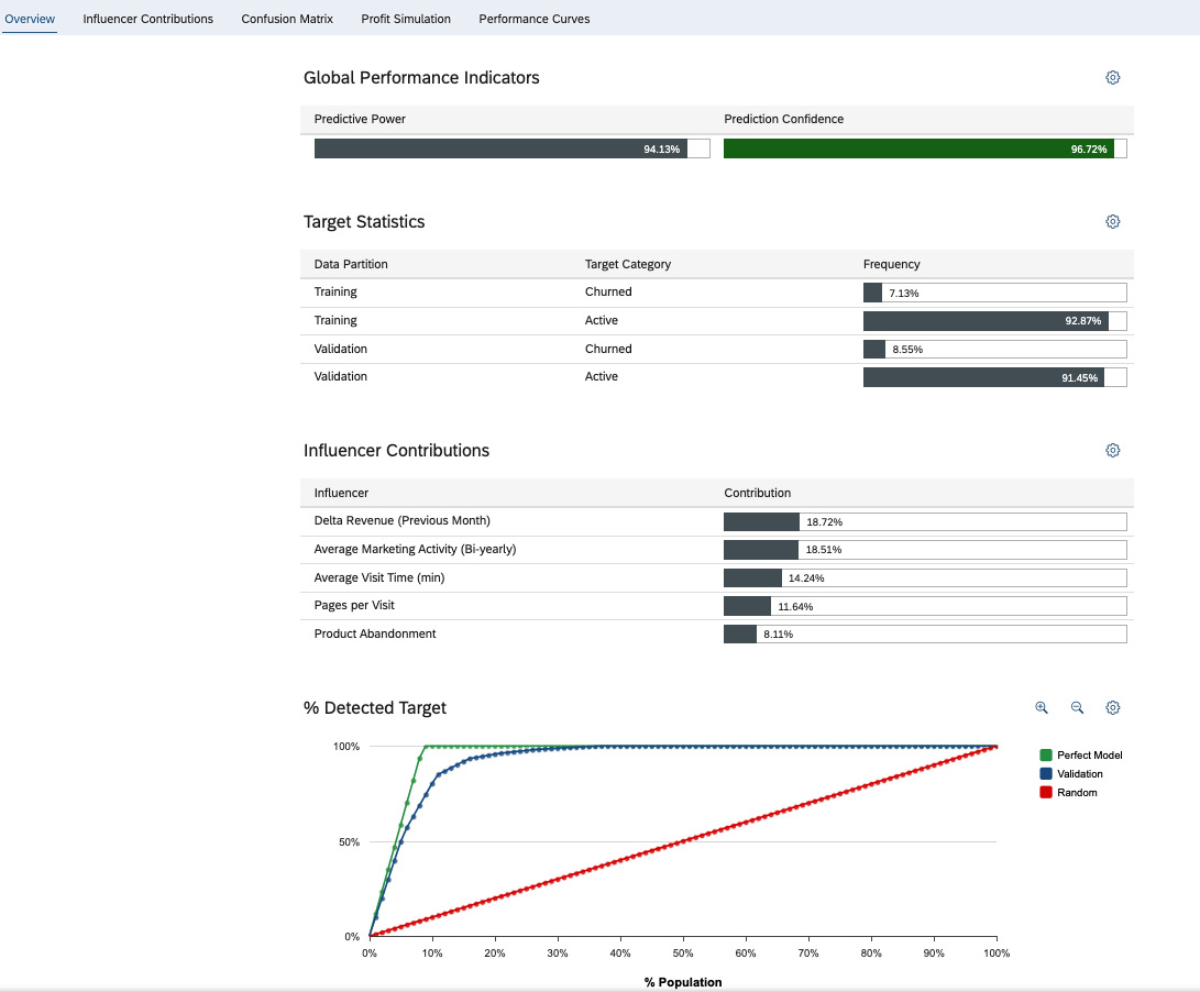
Figure 13.7 – Customer churn classification

Underneath, a classification predictive model uses Gradient Boosting trees to combine multiple week learners in an iterative process. Each iteration includes three steps. First, it calculates the residual for each case of the estimation dataset (75% of the dataset, which is used for training purposes). Second, it splits the estimation dataset on each variable and calculates the decision trees that predict the residual best based on the accuracy of the tree. Finally, it selects the tree with the highest gain for the next iteration and calculates a predicted value. This process stops when one of the conditions is satisfied and the final model is the combination of all winning trees – the trees with the highest gains.

Regression

Regression is used to predict the value of the target measure from historical data. For example, it is useful for answering questions about how much a customer will spend on a store, and how much revenue will be impacted by the new marketing campaign.

To predict, you will need the historical dataset, which represents the domain with a set of variables. For a regression model, the target variable must be numeric – a measure. In the example of a marketing campaign, the target variable can be the expected revenue resulting from the campaign based on other variables in the dataset such as promotions, country, customer type, and so on.

Regression in Smart Predict also relies on the Gradient Boosting technique to generate the best predictive model. The robustness of the regression model is also measured by prediction confidence. However, the quality of the regression model is measured by another indicator – the Root Mean Square Error (RMSE). The RMSE is calculated as the average of the square difference between the predicted and actual values for all cases of the validating dataset. The quality is better when the difference is smaller. RMSE is calculated with the following formula:

RMSE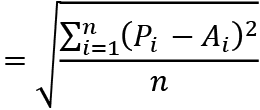

Here, n is the number of cases in the validation dataset, P is the predicted value, and A is the actual value of the case of the target.

The debrief information of a regression model includes two views. The overview page covers the performance indicator explained earlier, such as RMSE or prediction confidence, as well as the target statistics, and a summary of influence contributions. The Influence Contributions page lists the most important influencers, and how they positively or negatively influence the target. Knowing this will help users discover new insights and make better decisions. Figure 13.8 shows an example of the overview page for predicting sales opportunities:

Figure 13.8 – Sales opportunity regression

Time series forecasting

Time series models are used to forecast the future values of a time-dependent measure. For example, you can use time series forecasting to answer questions such as, what are the expected sales by products in the next few months?

For the dataset, it must have a time dimension and the values of the target variable in the past. The combination of the date and target variable is called a signal and will be analyzed by the predictive model. Depending on how far in the future you want to predict, typically, a 5:1 ratio is recommended for historical data and the prediction. For example, you can predict the next 2 months if 10 months of historical data is available. Here, the scale of the historical data and the prediction need to be the same. If the recorded historical data is more fine-grained, it is better to aggregate data in the unit of time you will need to predict. The other variables related to time are called candidate influencers – for example, the number of working days of a month, or specific events during the month such as holiday sales events. These candidate influencers are often domain-specific and have special meaning to detect certain components of signals, such as trends or cycles.

Technically, signals are broken down into four components:

• Trends: The first step is to determine the trend and the direction of the signal. The trend is either linear or quadratic for seasonal patterns. SAC Smart Predict tests eight trend models grouped into two groups:
  • Three stochastic methods that assume the forecast value will depend on the past values
  • Five deterministic methods that assume the forecast is independent of the past values and considers the candidate influencer variables
• Cycles: The second step is to determine the cycles, which represent the periodical and seasonal patterns. Cycles are computed by encoding the signal, either based on a period length or calendar events for seasonality. After that, it runs an iterative process for each of the eight detected trends to measure the links between the signal – the trend and the cycle – to see if it improves the forecast.
• Fluctuation: The third step is to determine the fluctuation of the signal after the trends and cycles have been extracted and use an auto-regression model to compute what is left on the signal.
• Residual: Finally, the remaining signals after trends, cycles, and fluctuation that are removed are considered noise – that is, random effects.

Figure 13.9 depicts the aforementioned process:

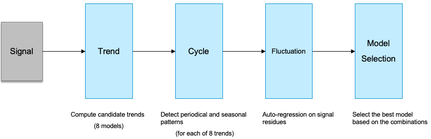
Figure 13.9 – Time series forecasting signal components

In the end, based on the determined components of the signal, SAC Smart Predict tries the combination of different models to find the best one, with the selected model whose residues are closest to white noise. To measure the performance of a model, the validation process compares the predicted values with the actual values based on a metric called Horizon-Wide Mean Absolute Percentage Error (MAPE), which is used as the quality indicator. MAPE measures the accuracy by comparing how much the forecast is different from the actual value. Horizon-Wide MAPE computes several individual MAPEs and calculates the average based on the requested horizon – how far you want to predict. A Horizon-Wide MAPE is computed with the following formula:

Horizon Wide MAPE (forecast, signal, H)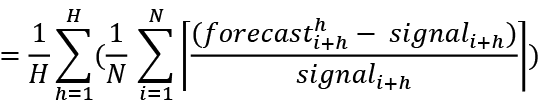

Here, forecast is the predicted value, signal is the actual value, h is the horizon (the number of periods in the future for prediction), and n is the number of items for the target variable.

If a predictive model has a Horizon-Wide MAPE near zero, it is a good model. Otherwise, you will need to apply your domain knowledge to determine the accuracy and check if it is applicable.

Using the predictive model

Once you have trained the predictive model and you are satisfied with the quality of the model, you can apply the predictive model and save the output into a dataset. Figure 13.10 shows how to apply a classification model based on the customer churn example we discussed previously:

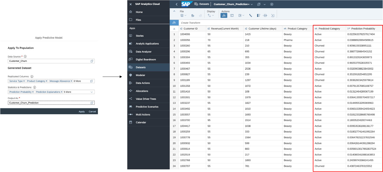
Figure 13.10 – Applying a predictive model

Once the output dataset is available, you can use it directly in a story, or create a model on top of the dataset and use it in a planning story.

Planning

For many companies, planning is one of the most critical and complex processes for their business operations and priorities. SAC offers full-fledged planning functionalities to support collaborative enterprise planning. This includes strategic and financial planning to set the overall direction at an aggregated level using planning assumptions, growth drives, profit and loss statements, balance sheets, and cash flow, as well as operational planning inside organizations such as sales, HR, and supplier chains and how they each impact the business results.

Planning in SAC is supported by a collaborative workflow. SAC addresses the collaboration challenges by providing collaborative and commenting functions. For example, you can create a planning calendar in SAC, where each task can be assigned to a planner that is responsible for it, and all the planners will be informed by the system of the assigned action items.

The Smart Predict features introduced previously can be used for predictive planning to create automated planning proposals that can be adjusted by experienced planners or enable planning with time series forecasting. SAC can disaggregate plan data to the raw data level, support distribution and spreading functions, or create advanced formulas using scripts.

Planning is all about connecting the various data from surrounding enterprise systems. For that, SAC can integrate master data and transactional data from SAP S/4HANA or populate the planning results back to S/4HANA. SAC can also integrate with SAP SuccessFactors for workforce planning in HR.

Important note

There are many more concepts, architectural considerations, and best practices about planning we cannot cover in this chapter. To learn more about planning with SAC, enroll in the open SAP course at https://open.sap.com/courses/sac3.

System landscapes and content life cycle management

In SAC, depending on the business needs, multiple environments can be provisioned, such as Sandbox, Dev, QA, Test Preview, and Prod. All these environments are updated on a scheduled basis by SAP as a managed SaaS offering. Multiple factors determine the landscape architecture, such as the test strategy, choice of public or private edition, integration with on-premise systems, and the life cycle and change management of content between environments.

SAC offers the choice of public and private hosted editions. For the public edition, a tenant is provisioned in a shared HANA database with a schema per customer. For the private edition, there are some other shared infrastructure components, but the HANA database is dedicated. If your business requires you to manage encryption keys with the Bring Your Own Key (BYOK) feature, then note it is only available with the private edition. In that case, an SAP Data Custodian key management service tenant is required for each SAC private tenant. Performance testing is only permitted in the private edition, while penetration testing can be requested for both editions. To request penetration testing, follow the process described in KBA 3080379 at https://launchpad.support.sap.com/#/notes/3080379.

Just like HANA Cloud and DWC, SAC follows a Quarterly Release Cycle (QRC) schedule. Within the QRC, SAC organizes the releases in waves; each wave occurs every 2 weeks. For example, Wave 2022.02 is the second wave as part of 2022.Q1 QRC. Dev, QA, and Prod all follow the same release schedule so that content can be transported between them without having to worry about versioning. The test preview environment is only available in the private edition, which receives the quarterly release around ~1 month earlier. This provides some customers with the opportunity to validate the new release with existing productive content. However, it should not be used for development or production purposes. For example, you cannot transport content from the test preview to other environments for the first month when its version is not aligned. Technically, there is also the Fast Track option, which is updated for each wave. It can be used as a Sandbox environment. Sandbox can only be used for testing purposes. Figure 13.11 summarizes the aforementioned release cycles for different environments:

Figure 13.11 – SAC release cycles

Some of the best practices for content life cycle management include the following:

• Follow the same update release cycle for the Dev, QA, and Prod environments.
• Validate content with production data; for example, use the test preview environment to validate new releases.
• Use Fast Track to test upcoming new features and plan your projects ahead of time.
• Only create an object once and transport it to different environments to keep the same ID and its dependencies.
• Make sure the content namespace is consistent across different environments. SAC APIs will refer to this content namespace.
• Use the Content Network to transport objects between environments without exporting/importing them.

Security concepts – users, roles, teams, and licenses

SAC organizes its security features around users, roles, teams, and licenses. A role can contain many users and a user can be in many roles. The role is the only place where you can define the application rights, such as create, update, or delete content types such as models or stories: a team can contain many users and a user can belong to many teams. Teams can be used as aggregators to group roles together; a user that belongs to a team inherits the rights that have been assigned to the roles of the team. Access rights to the folders in SAC are assigned by teams or users, not roles. For each project, SAC recommends that you create a project Folder and follow the same naming convention for the contents within the project folder.

Licenses are assigned to users through roles. The following license types are available; a single role can only consume one of the following license types:

• Business Intelligence: Named user
• Planning Standard: Named user; it includes a Business Intelligence – named user license
• Planning Profession: Named user; it includes a Planning Standard – named user license

In terms of BI, concurrent session licenses and Analytics Hub licenses that were previously available are no longer available for purchase. A single user can consume multiple licenses, but a user can only consume one of the BI licenses. For example, a Business Intelligence – concurrent session license cannot consume a planning license because the planning license includes the Business Intelligence – named user license.

The following are some general best practices for managing licenses with roles and teams:

• If you’re not using a user provisioning solution, it is recommended that you use a SAML2 IdP to map users to teams:
  • Enable dynamic user creation in the SAC setup
  • Use the SAM2 team user attribute to map with SAC teams, and use teams to group roles together
• If you’re using a user provisioning solution such as SAP Identity Provisioning, it is recommended that you create the users without any role. Instead, assign users to teams and assign roles to teams.

Administration Cockpit

Starting from the 2022.Q1 QRC release, the Administration Cockpit is available, which provides a consolidated view for all administrative tasks, including but not limited to authorization, dependencies, content sharing, usage analytics, tracing performance statistics, and many more. The Administration Cockpit itself is a SAC analytics application that is enabled by default in the system folder; users don’t need to import it from the Content Network.

Technically, the Administration Cockpit includes two parts – the main application, SAC_ADMIN_COCKPIT, and the fact sheets for detailed information. Together, they provide the following:

• A content summary for all content types in SAC such as folders, models, stories, applications, connections, dimensions, data actions, and more, grouped by general content or planning-related content.
• Authorization assignments of users, teams, and roles, as well as checking the teams without any user assignment, inactive users and users never used, and more.
• Sharing settings for folders, models, stories, and applications to understand who has access to a list of shared objects
• Allow you to understand the dependencies between objects and how models, connections, stories, and other objects are related to each other.
• Allow you to understand the usage of objects – for example, the top 10 used models, applications, and housekeeping help to identify objects that are not actively used.
• Tracing to show the error history and correlation, and the top 10 users with more errors.
• An end-to-end performance analysis tool based on the SAC_PERFORMANCE_TOOL analytics model, which shows page startup time and load time, the runtime distributions, backend processing statistics, network statistics, and frontend performance.
• Data action performance statistics and analysis based on the live data model, PLANNING_DATA_ACTIONS, shows the number of users who have scheduled or triggered data actions, the number of models with data actions, and how they are triggered or executed, such as the scheduling, median duration to complete, number of failures, and so on.
• Fact sheets for detailed information about a particular user, role, team, analytics application, story, connection, folder, dataset, and more.

Figure 13.12 shows the Administration Cockpit home page:

Figure 13.12 – The Administration Cockpit home page

The Administration Cockpit organizes the features mentioned earlier in the different tabs of the same application in SAC.

Performance Benchmark

Starting from the 2022.Q2 QRC release, SAC provides a Performance Benchmark to help customers understand and measure how performance can impact the user experience. It runs several scripts to calculate a normalized score of the client machine, or the network latency and bandwidth. Network performance impacting the speed of accessing SAC and downloading and uploading data can be negatively affected by network configurations such as VPC and firewall rules. Performance Benchmark can be accessed by going to System | Performance | Benchmark Tool. Figure 13.13 shows an example of this:

Figure 13.13 – Performance Benchmark

With this, we have a deeper understanding of SAC.

Summary

Thanks for staying with me. This was probably one of the longest chapters as we covered two major topics – DWC and SAC. This is because they are related to each other and, together, serve as the foundation for providing the necessary capabilities to turn data into insights and actions integrated into business processes.

We started this chapter by introducing DWC, its use cases, and the key concepts, such as Space. We also covered the various options regarding data integration – both federation and replication from on-premise and cloud data sources – and explained how DWC works with SAP BW through SAP BW Bridge, which is important for customers who have existing investments in SAP BW. After that, we discussed the different modeling capabilities, which include Data Builder for technical users and Business Builder for business users. We wrapped up the DWC section by explaining how to consume content from DWC in SAC.

Regarding SAC, we discussed the connectivity it offers, which includes both live connections and data acquisitions, the differences between datasets and models in data preparation, creating visualizations with stories, and the more interactive analytics applications. We also talked about embedded analytics and how it is different from enterprise analytics, as well as the SAC APIs for tenant and content management. One of the coolest things about SAC is its smart capabilities, which include Search to Insight, Smart Insights, Smart Discovery, and Smart Prediction. We also talked about the different predictive scenarios in smart prediction. Finally, we discussed the system landscapes, content life cycle management, security concepts, and the Administration Cockpit, which provides a one-stop hub for all administrative tasks.

In the next chapter, based on the knowledge of the ML/AI capabilities we covered regarding the smart features of SAC, we will extend the scope of the broader AI strategy and offerings from SAP’s portfolio. Before that, take a break so that you can enjoy the next chapter!