Chapter 16
Navigating 3D Models
The only tools you need to navigate 2D drawings are Pan and Zoom, which are simple to use. However, getting around 3D models can be a bit more challenging. This chapter will delve into how to navigate 3D models in the AutoCAD® 2014 program. (Please note that the AutoCAD LT® software doesn’t support these features.) You’ll learn various methods for visualizing and navigating 3D models, from selecting visual styles to using preset isometric views. You’ll also learn how to orbit into custom views and interactively navigate in perspective.
- Using visual styles
- Working with tiled viewports
- Navigating with the ViewCube
- Orbiting in 3D
- Using cameras
- Navigating with SteeringWheels
- Saving views
Using Visual Styles
Visual styles control the way models appear in each viewport. The default visual style is 2D Wireframe, which is what you have been using in previous chapters. Consider for a moment how 3D models are displayed on a 2D screen—an illusion. Creating the illusion of where objects are situated in space requires some visual indication as to which objects are in front of other occluded objects. A wireframe representation does not give this indication. Rather, occlusion objects need to be either hidden or covered by the shading of other objects according to the visual style that is selected.
Visual styles are never photorealistic like a rendering can be (see Chapter 18, “Presenting and Documenting 3D Design”), but many offer more realistic real-time views of your model compared to wireframe representations. In the following steps, you will sample the visual styles available in AutoCAD 2014.
The model in this chapter is a conceptual model of the O2 Arena in London that you will build in Chapter 17, “Modeling in 3D.” The O2 Arena (designed by architect Richard Rogers) was originally known as the Millennium Dome because it opened on January 1, 2000. This distinctive, mast-supported, dome-shaped cable network structure was one of the venues for the London 2012 Olympics (see Figure 16-1).
Symbolizing the number of days, weeks, and months in a year, the O2 Arena is 365 m in diameter and 52 m high, and is supported by 12 masts. It is also on the Prime Meridian that runs through Greenwich.
1. Go to the book’s web page at
www.sybex.com/go/autocad2014essentials, browse to Chapter 16, get the file
Ch16-A.dwg, and open it. The sample file is displayed in 2D Wireframe visual style by default.
2. Select the 3D Modeling workspace from the Quick Access toolbar.
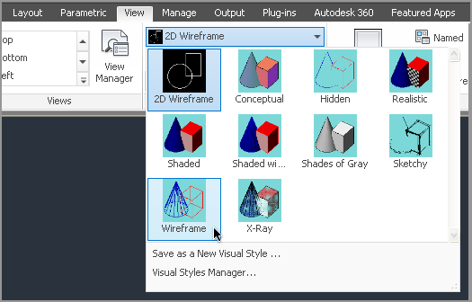
3. Select the ribbon’s View tab, and open the Visual Styles drop-down menu at the top of the Visual Styles panel (see
Figure 16-2).
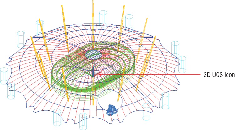
4. Select the Wireframe icon. The UCS icon displays a colorful axis tripod in this visual style (see
Figure 16-3).
You can change the uniform background color using the Colors button on the Display tab of the Options dialog box, invoked with the
OPTIONS command.
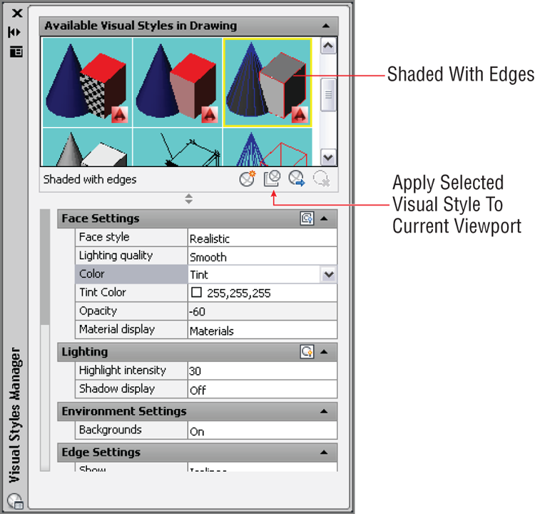
5. Select the Visual Styles Manager icon in the Palettes panel to alter visual style settings. Scroll down the list of Available Visual Styles In Drawing, and select Shaded With Edges. Change Color to Tint in the Face Settings group (see
Figure 16-4).
6. Select the Apply Selected Visual Style To Current Viewport button, as shown in
Figure 16-4. Close the Visual Styles Manager.
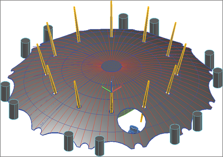
Figure 16-5 shows the result in the drawing canvas.
7. Open the Visual Styles drop-down menu in the Visual Styles panel, and select Save As A New Visual Style. The command prompt reads:
Save current visual style as or [?]:
Type Tinted with edges, and press Enter. These words appear on the Visual Styles drop-down menu, showing that this is now the current visual style.
By saving a visual style, you can recall it later after switching to another visual style.
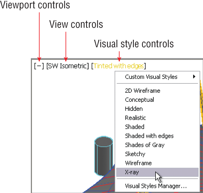
8. You can also change visual styles using the in-canvas controls located in the upper-left corner of the viewport. Select the Visual Style Controls to open a menu (see
Figure 16-6).
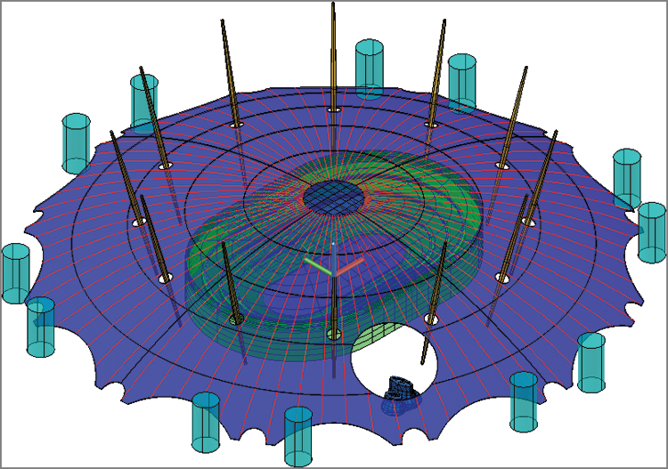
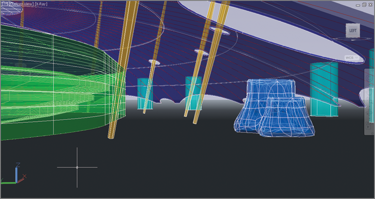
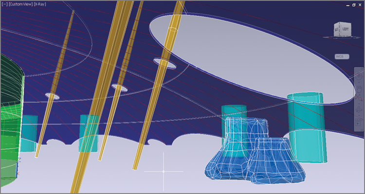
9. Choose X-ray from the in-canvas menu that appears.
Figure 16-7 shows the result: a transparent, shaded view with edges.
10. Save your work as Ch16-B.dwg.
Working with Tiled Viewports
Tiled viewports allow you to visualize a 3D model from different simultaneous vantage points. By starting a command in one viewport and finishing it in another, you can more easily transform objects in 3D. To help you get a better grasp of how this works, the following steps show you how to divide the single default viewport into three tiled viewports:
Tiled viewports can only exist in modelspace with the system variable
TILEMODE equal to 1. Floating viewports exist only on layouts.
1. If the file is not already open, go to the book’s web page, browse to Chapter 16, get the file Ch16-B.dwg, and open it.
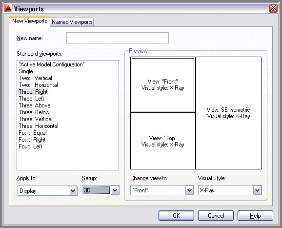
2. Type
VPORTS, and press Enter. In the Viewports dialog box that appears, select Three: Right in the Standard Viewports list. Open the Setup drop-down menu, and select 3D (see
Figure 16-8). Click OK.
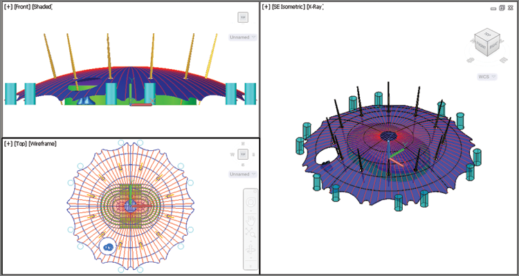
3. Click anywhere inside the viewport showing the front view to activate it. Open the in-canvas Visual Style Controls menu in this viewport and select Shaded. Click anywhere inside the viewport showing the top view to activate it. Open the in-canvas Visual Style Controls menu in this viewport and select Wireframe. Click OK.
Figure 16-9 shows the result.
4. Select the plus (+) symbol in the upper-left viewport displaying the front view to open the in-canvas Viewport menu. Select Maximize Viewport. The front view fills the drawing canvas.
You can maximize or minimize viewports as needed at any time to get a better view of a 3D object.
5. Observe that what was formerly a plus (+) symbol in the in-canvas Viewport menu is now a minus (–) symbol. Double-click the minus symbol to minimize this viewport, displaying the front view.
6. Click anywhere inside the right viewport showing the SE Isometric view to activate it. Double-click this viewport’s plus symbol to maximize it. The SE Isometric view once again fills the drawing canvas.
7. Save your work as Ch16-C.dwg.
Navigating with the ViewCube
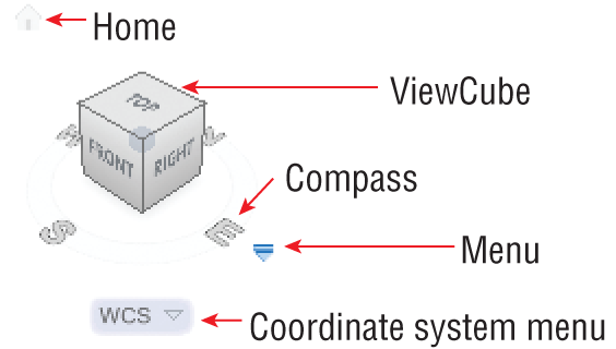
The ViewCube is a 3D navigation interface that lets you easily rotate through numerous preset orthogonal and isometric views. The ViewCube’s instant visual feedback keeps you from getting lost in 3D space, even when you orbit into a custom view.
The ViewCube helps you visualize the relationship between the current user coordinate system (UCS) and the world coordinate system (WCS).
In the following steps, you will experiment with the ViewCube and learn how to view a 3D model from almost any angle.
Autodesk uses the ViewCube and SteeringWheel navigation controls in many 3D applications, including AutoCAD, Autodesk
® Revit
®, Autodesk
® Inventor
®, and Autodesk
® 3ds Max
®.
1. If the file is not already open, go to the book’s web page, browse to Chapter 16, get the file Ch16-C.dwg, and open it.
2. Open the ViewCube menu (see
Figure 16-10), and select Set Current View As Home.
3. Hover your cursor over the ViewCube, and observe that different parts highlight in blue as you pass over them. Click the word Right. The view changes to an orthogonal view of the right side of the model (also known as an architectural elevation).
You can select from a short list of preset views using the in-canvas View Controls menu as an alternative to the ViewCube.
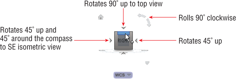
4. The ViewCube rotates with the view change. Hover the cursor over each of the elements on the right face and observe there are four corners, four edges, plus the right face itself that highlights in blue. In addition, there are four arrows facing the cube and two curved arrows in the upper right. Each of these interface elements rotates the view in a specific direction, as indicated in
Figure 16-11.
5. Spend some time navigating with the ViewCube, rotating into multiple different views. Try Bottom, Left, Back, SE Isometric, and NW Isometric.
6. Click the Home icon in the ViewCube interface to return to the initial view.
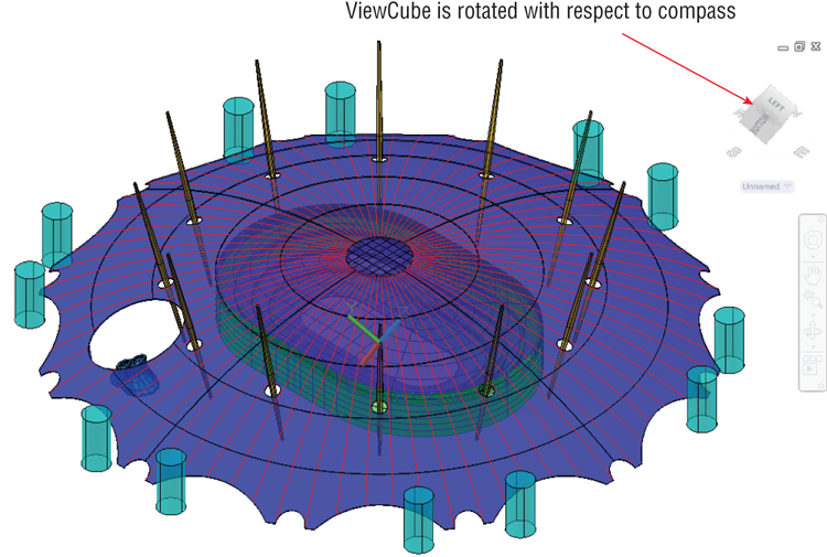
7. Select the UCS icon at the center of the 3D model to activate it. Drag the tip of the blue z-axis. The command prompt reads:
** Z AXIS DIRECTION **
Specify a point on Z axis:
Click an arbitrary point in the drawing canvas to rotate the UCS. Observe that the ViewCube rotates relative to the current UCS (see
Figure 16-12). This feedback can help you visualize where the XY drawing plane is (parallel to the Top face of the ViewCube).
8. Open the ViewCube’s Coordinate System menu, and select WCS to restore the original coordinate system.
9. Save your work as Ch16-D.dwg.
Orbiting in 3D
As you learned in the previous section, the ViewCube is limited to rotating the view in 45° increments. While the ViewCube might get you close to the angle from which you wish to view a 3D model, you will often need to orbit to the optimal viewing angle to see particular geometry best. Orbiting refers to rotating the view at any arbitrary angle. In the following steps, you will learn a few methods of orbiting in 3D:
1. If the file is not already open, go to the book’s web page, browse to Chapter 16, get the file Ch16-D.dwg, and open it.
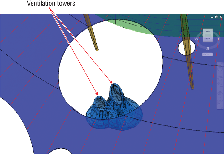
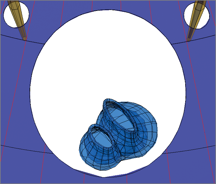
2. Let’s assume that you want to get a close look at the ventilation towers that appear under a large elliptical hole in the dome membrane. Click the edge between the Top and Front faces, and zoom into the ventilation towers, as shown in
Figure 16-13.
3. Position the cursor over the compass ring surrounding the ViewCube, and drag it to the right to get a better view of the ventilation towers so that the hole in the dome membrane appears more circular.
4. Click the Orbit tool in the Navigation bar. Drag down in the drawing canvas to orbit your point-of-view upward until you can see the ventilation towers unobstructed by the dome membrane (see
Figure 16-14). Press Esc to end the
3DORBIT command.
The Orbit tool is constrained so that it doesn’t roll by default. Use
3DFORBIT to orbit with roll.
5. Hold down Shift and drag the mouse wheel to orbit (without roll) about the ventilation towers once more. You will find that it is not possible to gain an eye-level view of the towers without other objects obstructing the view. You will learn how to set up this type of view using a camera in the next section.
6. Save your work as Ch16-E.dwg.
Using Cameras
AutoCAD uses virtual cameras to set up views similar to those achieved in the real world with physical cameras. The CAMERA command creates a camera object that you can manipulate in an isometric view to position the viewpoint in relation to the camera target. In the following steps, you will create a virtual camera and position it in an isometric view:
1. If the file is not already open, go to the book’s web page, browse to Chapter 16, get the file Ch16-E.dwg, and open it.
2. Open the in-canvas View Controls menu, and select SW Isometric.
3. Zoom out by rolling the mouse wheel backward.
4. Toggle off Object Snap in the status bar.
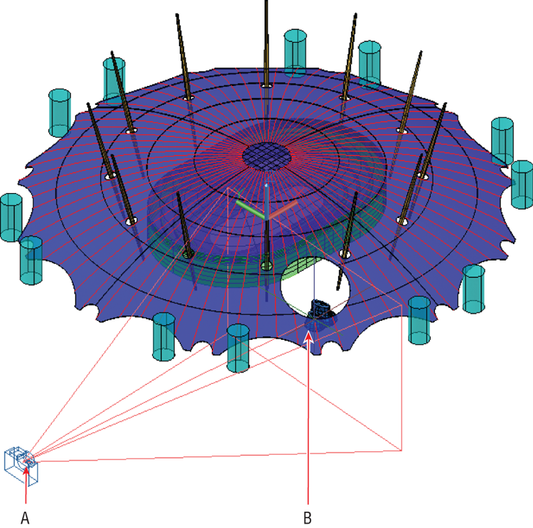
5. Type
CAMERA, and press Enter. Click points A and B, as shown in
Figure 16-15, and press Enter.
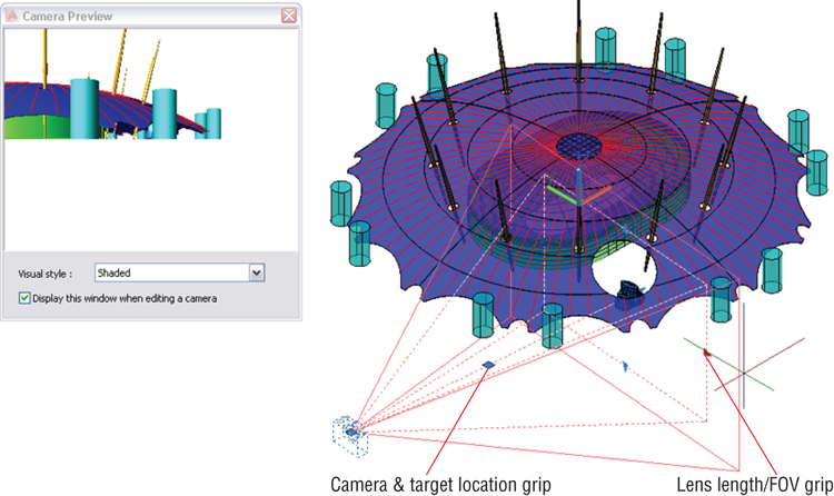
6. Select the camera object. Select the Shaded visual style in the Camera Preview window that appears. Drag the Lens Length/FOV grip to the right, and click approximately at point A to expand the field of view (see
Figure 16-16).
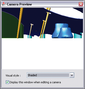
7. Drag the Camera & Target Location grip forward until the camera is under the outer edge of the dome.
Figure 16-17 shows the Camera Preview window. You will correct the fact that the camera is “on the ground” in the next step.
Camera views are in perspective so that objects diminish in size according to their distances from the camera.
8. Right-click in the drawing window, and choose Set Camera View. Drag the mouse wheel downward to move the camera and its target upward, as shown in
Figure 16-18.
9. Save your work as Ch16-F.dwg.
Navigating with SteeringWheels
The SteeringWheel is an interactive navigation control that Autodesk uses in many 3D applications, including AutoCAD. In the following steps, you will use the SteeringWheel’s full navigation wheel feature (displaying all eight navigation tools) to compose a view under the dome.
1. If the file is not already open, go to the book’s web page, browse to Chapter 16, get the file Ch16-F.dwg, and open it.
2. Select the SteeringWheel tool in the Navigation bar. The full navigation wheel appears in the drawing canvas in close proximity to the cursor (see
Figure 16-19).
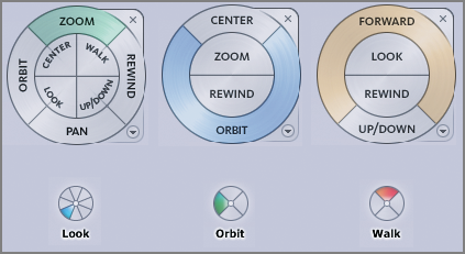
Additional SteeringWheels
There are eight commands that appear on variations of SteeringWheels: Zoom, Pan, Orbit, Rewind, Center, Walk, Up/Down, and Look.
There are three basic SteeringWheels: Full Navigation, View Object, and Tour Building. The latter two wheels have four commands—each command is suitable to its purpose of navigating around an object or touring through a building.
Each one of the basic wheels has a corresponding mini-wheel with the same commands as the larger interface. I suggest starting with the basic wheels and then graduating to mini-wheels as you gain experience. Mini-wheels are more efficient because you don't have to move the mouse as far to select navigation commands.
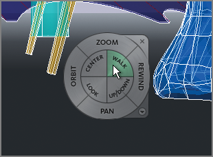
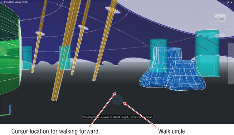
3. Position the cursor over the Walk tool within the inner ring of the SteeringWheel. Click and hold the mouse button, and observe a walk circle appear in the lower portion of the drawing canvas. Drag the cursor relative to the walk circle to move in that direction (see
Figure 16-20). The further from the walk circle you drag, the faster you walk in that direction. Release the mouse button.
4. Position the cursor over the Look tool in the SteeringWheel’s inner ring. Click and hold the mouse button, and drag upward to rotate the camera to look up at the hole in the dome above the ventilation towers. Release the mouse button.
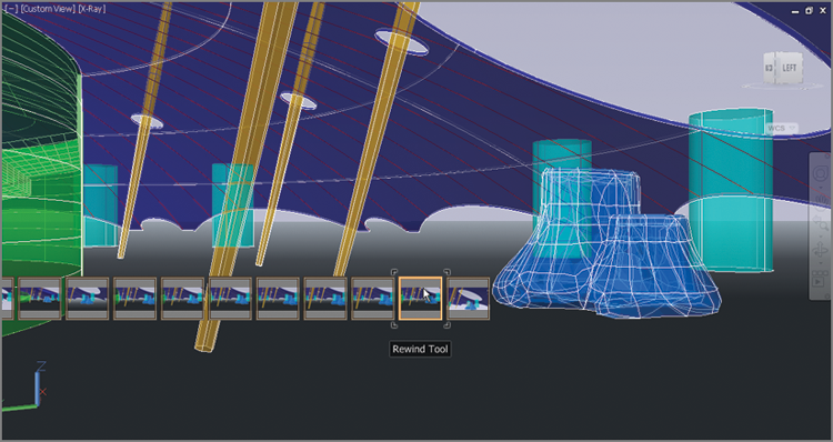
5. Position the cursor over the Rewind tool in the SteeringWheel’s outer ring. Drag to the left to go backward in the history of movements made using the steering wheel. Drag back to the point before you looked up (see
Figure 16-21). Press Esc to exit the SteeringWheel.
6. Save your work as Ch16-G.dwg.
Saving Views
Named views allow you to save where you are in space so that you can recall these positions in the future. In the following steps, you will save the current position in the viewport, change the view, switch out of perspective, and then return to the saved view:
1. If the file is not already open, go to the book’s web page, browse to Chapter 16, get the file Ch16-G.dwg, and open it.
2. Type V (for view), and press Enter. Click the New button in the View Manager dialog box that appears.
Many different properties can be saved with views, including Camera Position, Layer Snapshot, UCS, Live Section, Visual Style, and Background.
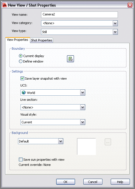
3. In the New View / Shot Properties dialog box that appears, type
Camera2 as the view name (see
Figure 16-22). Click OK twice to close both open dialog boxes.
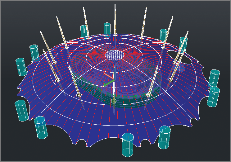
4. Click the upper-left corner of the left face of the ViewCube to switch to the NW Isometric view. The model is still in perspective even after switching out of the Camera2 view (see
Figure 16-23).
5. You can toggle in and out of perspective view at any time. Open the in-canvas View Controls menu, and select Parallel to switch out of perspective.
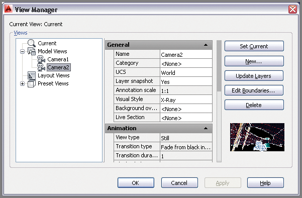
6. Type
V (for view), and press Enter. Select Camera2 in the list of Model Views in the View Manager dialog box (see
Figure 16-24). Click Set Current, Apply, and then OK. The initial perspective view is restored.
7. Save your work as
Ch16-H.dwg.
Figure 16-25 shows the result.
The Essentials and Beyond
In this chapter, you learned how to view a 3D model in a variety of ways, including changing its visual styles and working with tiled viewports. You also picked up important 3D navigation skills using the ViewCube, SteeringWheel, and 3DORBIT command. In addition, you placed a camera, adjusted its position and field of view in Isometric mode, looked through its virtual lens, and walked around an interior building space. Finally, you learned how to save and restore views so that you can get back to the places the virtual camera has been.
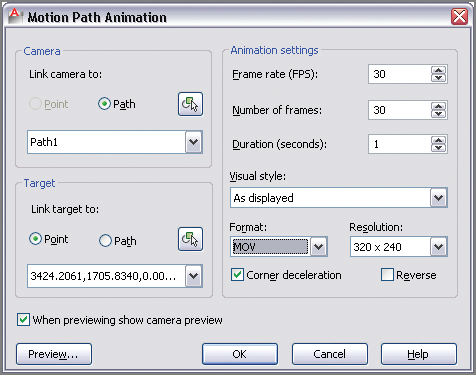
Additional Exercise
Did you know AutoCAD can create walkthrough and/or flyby animations? First draw a spline to act as a camera motion path. Edit the spline (see Chapter 5, “Shaping Curves,” if necessary) so that the spline has a smooth 3D shape. Use the ANIPATH command to create a motion path animation, linking the camera’s path to the spline you just drew. Export the animation to your hard drive and watch the video. You can share video files with people who don’t have AutoCAD.