One of the main limitations of the basic sorting algorithms is the amount of effort they require to move items that are a long way from their final sorted position into the correct place in the sorted result. The advanced sorting algorithms covered in this chapter give you the capability to move items a long way quickly, which is why they are far more effective at dealing with larger sets of data than the algorithms covered in the previous chapter.

Shellsort achieves this feat by breaking a large list of items into many smaller sublists, which are sorted independently using an insertion sort (see Chapter 6). While this sounds simple, the trick lies in repeating this process several times with careful creation of larger and larger sublists, until the whole list is sorted using an insertion sort on the final pass. As you learned in the previous chapter, an insertion sort is very effective on nearly sorted data, and this is exactly the state of the data on the final pass of a shellsort.

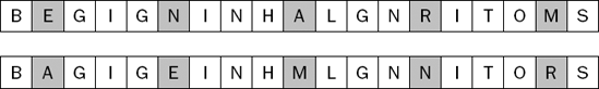
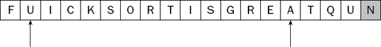
This shellsort example sorts the letters shown in Figure 7-1 alphabetically.

Figure 7.1. Sample data to demonstrate shellsort.

Shellsort is built upon the concept of H-sorting. A list is said to be H-sorted when, starting at any position, every H-th item is in sorted position relative to the other items. That concept will become clear as you work through an example. In the following Try It Out, you start by 4-sorting the list from Figure 7-1. In other words, you will consider only every fourth element and sort those items relative to each other.

Figure 7-2 shows every fourth item starting at position 0.

Figure 7.2. Every fourth item starting at position 0.

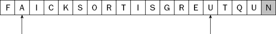
Ignoring all other items, you sort the highlighted items relative to each other, resulting in the list shown in Figure 7-3. The highlighted items now appear in alphabetical order (B, G, H, N, O).

Figure 7.3. Every fourth item starting at position 0 sorted relative to each other.

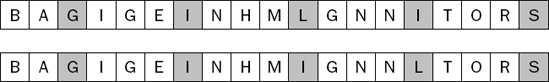
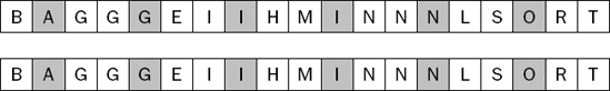
You now consider every fourth item starting at position 1. Figure 7-4 shows these items before and after they are sorted relative to each other.

Figure 7.4. Sorting every fourth item starting at position 1.

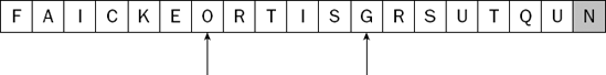
Next you 4-sort starting at position 2, as shown in Figure 7-5.

Figure 7.5. Sorting every fourth item starting at position 2.

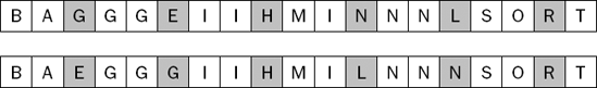
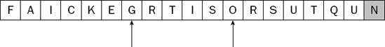
Finally, you consider every fourth item starting at position 3. Figure 7-6 shows the situation before and after this step.

Figure 7.6. Sorting every fourth item starting at position 3.

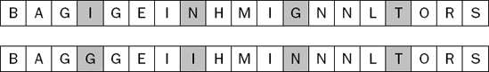
There is no more to do to 4-sort the sample list. If you were to move to position 4, then you would be considering the same set of objects as when you started at position 0. As you can see from the second line in Figure 7-6, the list is by no means sorted, but it is 4-sorted. You can test this by choosing any item in the list and verifying that it is less than (or equal to) the item four positions to its right, and greater than (or equal to) the item four positions to its left.

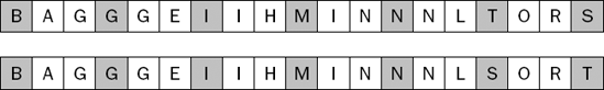
The shellsort moves items a long way quickly. For very large lists of items, a good shellsort would start with a very large value of H, so it might start by 10,000-sorting the list, thereby moving items many thousands of positions at a time, in an effort to get them closer to their final sorted position quickly. Once the list is H-sorted for a large value of H, shellsort then chooses a smaller value for H and does the whole thing again. This process continues until the value of H is 1, and the whole list is sorted on the final pass. In this example, you 3-sort the list for the next pass.

Figure 7-7 shows every third item starting at position 0, both before and after being sorted relative to each other. By the way, notice the arrangement of the last four letters!

Figure 7.7. 3-sorting at position 0.

You move to position 1, and by coincidence there is nothing to do, as shown in Figure 7-8.

Figure 7.8. 3-sorting at position 1.

Finally, you sort every third item starting at position 2, as shown in Figure 7-9.

Figure 7.9. 3-sorting at position 2.

Notice how the list is now nearly sorted. Most items are only a position or two away from where they should be, which you can accomplish with a simple insertion sort. After a quick run over the list, you end up with the final sorted arrangement shown in Figure 7-10. If you compare this with the previous list, you will see that no item had to move more than two positions to reach its final position.

Figure 7.10. The final sorted list.

Much of the research into shellsort has revolved around the choice of the successive values for H. The original sequence suggested by the algorithm's inventor (1, 2, 4, 8, 16, 32, . . .) is provably terrible, as it compares only items in odd positions with items in odd positions until the final pass. Shellsort works well when each item is sorted relative to different items on each pass. A simple and effective sequence is (1, 4, 13, 40, . . .) whereby each value of H = 3 × H + 1. In the following Try It Out, you implement a shellsort.

The test for your shellsort algorithm should look familiar by now. It simply extends AbstractListSorterTest and instantiates the (not yet written) shellsort implementation:

package com.wrox.algorithms.sorting;

public class ShellsortListSorterTest extends AbstractListSorterTest {
    protected ListSorter createListSorter(Comparator comparator) {
        return new ShellsortListSorter(comparator);
    }
}

package com.wrox.algorithms.sorting;

import com.wrox.algorithms.lists.List;

public class ShellsortListSorter implements ListSorter {
    private final Comparator _comparator;
    private final int[] _increments = {121, 40, 13, 4, 1};

    public ShellsortListSorter(Comparator comparator) {
        assert comparator != null : "comparator cannot be null";
        _comparator = comparator;
    }
    ...
}

public List sort(List list) {
        assert list != null : "list cannot be null";

        for (int i = 0; i < _increments.length; i++) {
            int increment = _increments[i];
            hSort(list, increment);
        }

        return list;
    }

private void hSort(List list, int increment) {
        if (list.size() < (increment * 2)) {
            return;
        }

        for (int i=0; i< increment; ++i) {
            sortSublist(list, i, increment);
        }
    }

private void sortSublist(List list, int startIndex, int increment) {
        for (int i = startIndex + increment; i < list.size(); i += increment) {
            Object value = list.get(i);
            int j;
            for (j = i; j > startIndex; j -= increment) {
                Object previousValue = list.get(j - increment);
                if (_comparator.compare(value, previousValue) >= 0) {
                    break;
                }
                list.set(j, previousValue);
            }
            list.set(j, value);
        }
    }

Quicksort is the first sorting algorithm discussed that uses recursion. Although it can be recast in an iterative implementation, recursion is the natural state for quicksort. Quicksort works using a divide-and-conquer approach, recursively processing smaller and smaller parts of the list. At each level, the goal of the algorithm is three-fold:

By maintaining these invariants in each pass, the list is divided into two parts (note that it is not necessarily divided into two halves) that can each be sorted independently of the other. This section uses the list of letters shown in Figure 7-11 as sample data.

Figure 7.11. Sample list for quicksort.

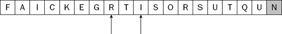
The first step in quicksort is to choose the partitioning item. This is the item that ends up in its final sorted position after this pass, and partitions the list into sections, with smaller items to the left (arranged randomly) and larger items to its right (arranged randomly). There are many ways to choose the partitioning item, but this example uses a simple strategy of choosing the item that happens to be at the far right of the list. In Figure 7-12, this item is highlighted. You also initialize two indexes at the leftmost and rightmost of the remaining items, as shown in the figure.

Figure 7.12. Starting position for the initial quicksort pass.

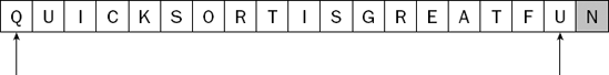
The algorithm proceeds by advancing the left and right indexes towards each other until they meet. As the left index proceeds, it stops when it finds an item that is larger than the partitioning item. As the right index proceeds, it stops when it encounters an item that is smaller than the partitioning item. The items are then swapped so that they are each in the appropriate part of the list. Remember that the idea is to have smaller items to the left and larger items to the right, although not necessarily in sorted order.

In the example shown in Figure 7-12, the left index is pointing to the letter Q. This is larger than the partitioning value (N), so it is out of place at the far left of the list. The right index was initially pointing at U, which is larger than N, so that's okay. If it moves one position to the left, it is pointing at the letter F, which is smaller than N. It is therefore out of place at the far right of the list. This situation is displayed in Figure 7-13.

Figure 7.13. The first two out-of-place items have been found.

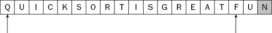
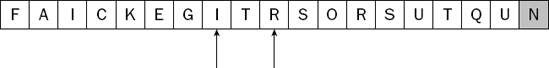
To get these two out-of-place items closer to their final sorted position, you swap them as shown in Figure 7-14.

Figure 7.14. The first two out-of-place items are swapped.

The left index now continues moving to the right until it encounters an item that is larger than the partitioning item. One is found immediately in the second position (U). The right index then proceeds moving to the left and finds an A out of place, as shown in Figure 7-15.

Figure 7.15. Two more out-of-place items are found.

Once again, the items are swapped, as shown in Figure 7-16.

Figure 7.16. The second pair of out-of-place items are swapped.

The same procedure continues as the left and right indexes move toward each other. The next pair of out-of-place items are S and E, as shown in Figure 7-17.

Figure 7.17. Two more out-of-place items are found.

You swap these items, leaving the list in the state shown in Figure 7-18. At this stage, every item to the left of the left index is less than the partitioning item, and every item to the right of the right index is larger than the partitioning item. The items between the left and right indexes still need to be handled.

Figure 7.18. The letters E and S are swapped.

You continue with the same procedure. The next out-of-place items are shown in Figure 7-19.

Figure 7.19. The letters O and G are out of place.

You swap them into the position shown in Figure 7-20.

Figure 7.20. The letters O and G are swapped.

You are almost done for the first quicksort pass. Figure 7-21 demonstrates that one pair of out-of-place items remain.

Figure 7.21. The letters R and I are out of place.

After you swap them, the list is in the state shown in Figure 7-22.

Figure 7.22. The letters R and I are swapped.

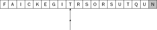
Now things get interesting. The algorithm proceeds as before, with the left index advancing until it finds an item larger than the partitioning item, in this case the letter T. The right index then advances to the left but stops when it reaches the same value as the left index. There is no advantage to going beyond this point, as all items to the left of this index have been dealt with already. The list is now in the state shown in Figure 7-23, with both left and right indexes pointing at the letter T.

Figure 7.23. The left and right indexes meet at the partitioning position.

The point where the two indexes meet is the partitioning position—that is, it is the place in the list where the partitioning value actually belongs. Therefore, you do one final swap between this location and the partitioning value at the far right of the list to move the partitioning value into its final sorted position. When this is done, the letter N is in the partitioning position, with all of the values to its left being smaller, and all of the values to its right being larger (see Figure 7-24).

Figure 7.24. The partitioning item in final sorted position.

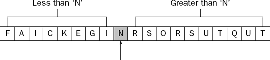
All the steps illustrated so far have resulted in only the letter N being in its final sorted position. The list itself is far from sorted. However, the list has been divided into two parts that can be sorted independently of each other. You simply sort the left part of the list, and then the right part of the list, and the whole list is sorted. This is where the recursion comes in. You apply the same quicksort algorithm to each of the two sublists to the left and right of the partitioning item.

You have two cases to consider when building recursive algorithms: the base case and the general case. For quicksort, the base case occurs when the sublist to be sorted has only one element; it is by definition already sorted and nothing needs to be done. The general case occurs when there is more than one item, in which case you apply the preceding algorithm to partition the list into smaller sublists after placing the partitioning item into the final sorted position.

Having seen an example of how the quicksort algorithm works, you can test it in the next Try It Out exercise.

package com.wrox.algorithms.sorting;

public class QuicksortListSorterTest extends AbstractListSorterTest {
    protected ListSorter createListSorter(Comparator comparator) {
        return new QuicksortListSorter(comparator);
    }
}

package com.wrox.algorithms.sorting;

import com.wrox.algorithms.lists.List;

public class QuicksortListSorter implements ListSorter {
    private final Comparator _comparator;

    public QuicksortListSorter(Comparator comparator) {
        assert comparator != null : "comparator cannot be null";
        _comparator = comparator;
    }
    ...
}

public List sort(List list) {
        assert list != null : "list cannot be null";

        quicksort(list, 0, list.size() − 1);

        return list;
    }

private void quicksort(List list, int startIndex, int endIndex) {
        if (startIndex < 0 || endIndex >= list.size()) {
            return;
        }
        if (endIndex <= startIndex) {
            return;
        }

        Object value = list.get(endIndex);

        int partition = partition(list, value, startIndex, endIndex − 1);
        if (_comparator.compare(list.get(partition), value) < 0) {
            ++partition;
        }

        swap(list, partition, endIndex);

        quicksort(list, startIndex, partition − 1);
        quicksort(list, partition + 1, endIndex);
    }

private int partition(List list, Object value, int leftIndex, int rightIndex) {
        int left = leftIndex;
        int right = rightIndex;

        while (left < right) {
            if (_comparator.compare(list.get(left), value) < 0) {
                ++left;
                continue;
            }

            if (_comparator.compare(list.get(right), value) >= 0) {
                −−right;
                continue;
            }

            swap(list, left, right);
            ++left;
        }

        return left;
    }

private void swap(List list, int left, int right) {
        if (left == right) {
            return;
        }
        Object temp = list.get(left);
        list.set(left, list.get(right));
        list.set(right, temp);
    }

Before considering the third advanced sorting algorithm, this section elaborates on the discussion of stability, which was first brought to your attention in the previous chapter. Now is a good time because the two algorithms discussed so far in this chapter share the shortcoming that they are not stable. The algorithm covered next—mergesort—is stable, so now is a good opportunity to deal with the lack of stability in shellsort and quicksort.

As you learned in Chapter 6, stability is the tendency of a sorting algorithm to maintain the relative position of items with the same sort key during the sort process. Quicksort and shellsort lack stability, as they pay no attention at all to the items that are near each other in the original input list. This section discusses a way to compensate for this issue when using one of these algorithms: the compound comparator.

The example in Chapter 6 was based on a list of people that was sorted by either first name or last name. The relative order of people with the same last name is maintained (that is, they were ordered by first name within the same last name group) if the algorithm used is stable. Another way to achieve the same effect is to use a compound key for the person object, consisting of both the first name and last name when sorting by first name, and both the last name and first name when sorting by last name. As you saw in Chapter 6, it is often possible to create useful general-purpose comparators to solve many different problems. That is the approach taken in the next Try It Out, where you create a compound comparator that can wrap any number of standard single-value comparators to achieve a sort outcome based on a compound key.

package com.wrox.algorithms.sorting;

public class FixedComparator implements Comparator {
    private final int _result;

    public FixedComparator(int result) {
        _result = result;
    }

    public int compare(Object left, Object right) {
        return _result;
    }
}

You can now begin writing tests for the compound comparator. You have to cover three basic cases: it returns zero, it returns a positive integer, or it returns a negative integer from its compare() method. Each of these tests adds multiple fixed comparators to the compound comparator. The first of these is set up to return zero, indicating that the compound comparator must use more than the first element of the compound key to sort the items. The code for the three test cases is shown here:

package com.wrox.algorithms.sorting;

import junit.framework.TestCase;

public class CompoundComparatorTest extends TestCase {
    public void testComparisonContinuesWhileEqual() {
        CompoundComparator comparator = new CompoundComparator();
        comparator.addComparator(new FixedComparator(0));
        comparator.addComparator(new FixedComparator(0));
        comparator.addComparator(new FixedComparator(0));

        assertTrue(comparator.compare("IGNORED", "IGNORED") == 0);
    }

    public void testComparisonStopsWhenLessThan() {
        CompoundComparator comparator = new CompoundComparator();
        comparator.addComparator(new FixedComparator(0));
        comparator.addComparator(new FixedComparator(0));
        comparator.addComparator(new FixedComparator(-57));
        comparator.addComparator(new FixedComparator(91));

        assertTrue(comparator.compare("IGNORED", "IGNORED") < 0);
    }

    public void testComparisonStopsWhenGreaterThan() {
        CompoundComparator comparator = new CompoundComparator();

comparator.addComparator(new FixedComparator(0));
        comparator.addComparator(new FixedComparator(0));
        comparator.addComparator(new FixedComparator(91));
        comparator.addComparator(new FixedComparator(-57));

        assertTrue(comparator.compare("IGNORED", "IGNORED") > 0);
    }
}

package com.wrox.algorithms.sorting;

import com.wrox.algorithms.iteration.Iterator;
import com.wrox.algorithms.lists.ArrayList;
import com.wrox.algorithms.lists.List;

public class CompoundComparator implements Comparator {
    private final List _comparators = new ArrayList();
    ...
}

public void addComparator(Comparator comparator) {
        assert comparator != null : "comparator can't be null";
        assert comparator != this : "can't add comparator to itself";

        _comparators.add(comparator);
    }

public int compare(Object left, Object right) {
        int result = 0;
        Iterator i = _comparators.iterator();

        for (i.first(); !i.isDone(); i.next()) {
            result = ((Comparator) i.current()).compare(left, right);
            if (result != 0) {
                break;
            }
        }

        return result;
    }

Mergesort is the last of the advanced sorting algorithms covered in this chapter. Like quicksort, it is possible to implement mergesort both recursively and iteratively, but we implement it recursively in this section. Unlike quicksort, mergesort does not sort the list it is provided in place; rather, it creates a new output list containing the objects from the input list in sorted order.

Merging

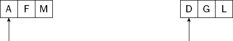
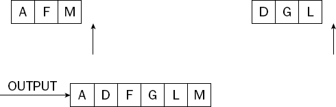
Mergesort is built upon the concept of merging. Merging takes two (already sorted) lists and produces a new output list containing all of the items from both lists in sorted order. For example, Figure 7-25 shows two input lists that need to be merged. Note that both lists are already in sorted order.

Figure 7.25. Two already sorted lists that we want to merge.

The process of merging begins by placing indexes at the head of each list. These will obviously point to the smallest items in each list, as shown in Figure 7-26.

Figure 7.26. Merging begins at the head of each list.

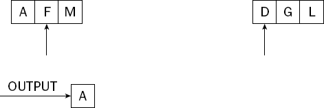
The items at the start of each list are compared, and the smallest of them is added to the output list. The next item in the list from which the smallest item was copied is considered. The situation after the first item has been moved to the output list is shown in Figure 7-27.

Figure 7.27. The first item is added to the output list.

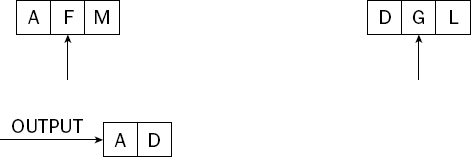
The current items from each list are compared again, with the smallest being placed on the output list. In this case, it's the letter D from the second list. Figure 7-28 shows the situation after this step has taken place.

Figure 7.28. The second item is added to the output list.

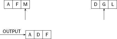
The process continues; this time the letter F from the first list is the smaller item and it is copied to the output list, as shown in Figure 7-29.

Figure 7.29. The third item is placed on the output list.

This process continues until both input lists have been exhausted and the output contains each item from both lists in sorted order. The final state is shown in Figure 7-30.

Figure 7.30. The completed merge process.

The mergesort Algorithm

The mergesort algorithm is based upon the idea of merging. As with the quicksort algorithm, you approach mergesort with recursion, but quicksort was a divide-and-conquer approach, whereas the mergesort algorithm describes more of a combine-and-conquer technique. Sorting happens at the top level of the recursion only after it is complete at all lower levels. Contrast this with quicksort, where one item is placed into final sorted position at the top level before the problem is broken down and each recursive call places one further item into sorted position.

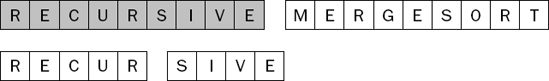
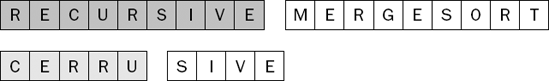
This example uses the list of letters shown in Figure 7-31 as the sample data.

Figure 7.31. Sample list to demonstrate recursive mergesort.

Like all the sorting algorithms, mergesort is built upon an intriguingly simple idea. Mergesort simply divides the list to be sorted in half, sorts each half independently, and merges the result. It sounds almost too simple to be effective, but it will still take some explaining. Figure 7-32 shows the sample list after it has been split in half. When these halves are sorted independently, the final step will be to merge them together, as described in the preceding section on merging.

Figure 7.32. The sample list when split in half.

A key difference between mergesort and quicksort is that the way in which the list is split in mergesort is completely independent of the input data itself. Mergesort simply halves the list, whereas quicksort partitions the list based on a chosen value, which can split the list at any point on any pass.

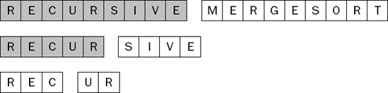
So how do you sort the first half of the list? By applying mergesort again! You split that half in half, sort each half independently, and merge them. Figure 7-33 shows half of the original list split in half itself.

Figure 7.33. The first recursive call to mergesort the first half of the original list.

How do you sort the first half of the first half of the original list? Another recursive call to mergesort, of course. By now you will no doubt be getting the idea that you keep recursing until you reach a sublist with a single item in it, which of course is already sorted like any single-item list, and that will be the base case for this recursive algorithm. You saw the general case already—that is, when there is more than one item in the list to be sorted, split the list in half, sort the halves, and then merge them together.

Figure 7-34 shows the situation at the third level of recursion.

Figure 7.34. Third level of recursion during mergesort.

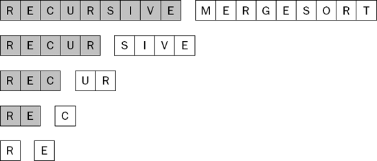
As you still have not reached a sublist with one item in it, you continue the recursion to yet another level, as shown in Figure 7-35.

Figure 7.35. Fourth level of recursion during mergesort.

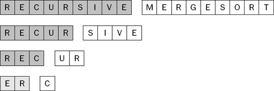
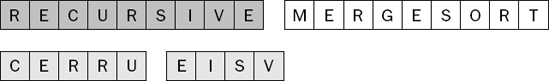
At the level of recursion shown in Figure 7-35, you are trying to sort the two-element sublist containing the letters R and E. This sublist has more than one item in it, so once more you need to split and sort the halves as shown in Figure 7-36.

Figure 7.36. The final level of recursion in the mergesort example.

You have finally reached a level at which you have two single-item lists. This is the base case in the recursive algorithm, so you can now merge these two single-item sorted lists together into a single two-item sorted sublist, as shown in Figure 7-37.

Figure 7.37. The first merge operation is complete.

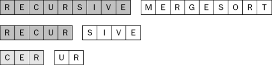
In Figure 7-37, the two sublists of the sublist (R, E, C) are already sorted. One is the two-element sublist you just merged, and the other is a single-item sublist containing the letter C. These two sublists can thus be merged to produce a three-element sorted sublist, as shown in Figure 7-38.

Figure 7.38. The second merge operation is complete.

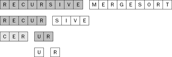
The sublist (R, E, C, U, R) now has one sublist that is sorted and one sublist that is not yet sorted. The next step is to sort the second sublist (U, R). As you would expect, this involves recursively mergesorting this two-element sublist, as shown in Figure 7-39.

Figure 7.39. Recursively sorting the (U, R) sublist.

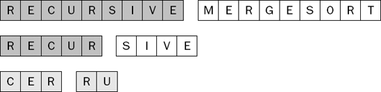
The two single-item sublists can now be merged as shown in Figure 7-40.

Figure 7.40. Merging the two single-item sublists.

Both sublists of the (R, E, C, U, R) sublist are sorted independently, so the recursion can unwind by merging these two sublists together, as shown in Figure 7-41.

Figure 7.41. Unwinding the recursion by merging two sublists.

The algorithm continues with the (S, I, V, E) sublist until it too is sorted, as shown in Figure 7-42. (We have skipped a number of steps between the preceding and following figures because they are very similar to the steps for sorting the first sublist.)

Figure 7.42. Ready to merge the first half of the original list.

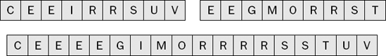
The final step in sorting the first half of the original list is to merge its two sorted sublists, giving the result shown in Figure 7-43.

Figure 7.43. The first half of the list is now sorted.

The algorithm continues in exactly the same way until the right half of the original list is also sorted, as shown in Figure 7-44.

Figure 7.44. The right half of the original list is sorted.

Finally, you can merge the two sorted halves of the original list to form the final sorted list, as shown in Figure 7-45.

Figure 7.45. The final result.

Mergesort is an elegant algorithm that is relatively simple to implement, as you will see in the next Try It Out.

Try It Out: Testing the Mergesort Algorithm

The test for the mergesort algorithm is the same as each of the other tests in this chapter, with the only difference being that you instantiate the appropriate implementation class:

package com.wrox.algorithms.sorting;

public class MergesortListSorterTest extends AbstractListSorterTest {
    protected ListSorter createListSorter(Comparator comparator) {
        return new MergesortListSorter(comparator);
    }
}

In the next Try It Out, you implement the mergesort.

Try It Out: Implementing Mergesort

Once again, the implementation follows the usual pattern: You implement the ListSorter interface and accept a comparator to impose order on the items to be sorted:

package com.wrox.algorithms.sorting;

import com.wrox.algorithms.lists.List;
import com.wrox.algorithms.lists.ArrayList;
import com.wrox.algorithms.iteration.Iterator;

public class MergesortListSorter implements ListSorter {
    private final Comparator _comparator;

    public MergesortListSorter(Comparator comparator) {
        assert comparator != null : "comparator cannot be null";
        _comparator = comparator;
    }
    ...
}

You use the sort() method from the ListSorter interface to call the mergesort() method, passing in the lowest and highest item indexes so that the entire list is sorted. Subsequent recursive calls pass in index ranges that restrict the sorting to smaller sublists:

public List sort(List list) {
        assert list != null : "list cannot be null";

        return mergesort(list, 0, list.size() − 1);
    }

Create the mergesort() method that follows to deal with situations in which it has been called to sort a sublist containing a single item. In this case, it creates a new result list and adds the single item to it, ending the recursion.

If there is more than one item in the sublist to be sorted, the code simply splits the list, recursively sorts each half, and merges the result:

private List mergesort(List list, int startIndex, int endIndex) {
        if (startIndex == endIndex) {
            List result = new ArrayList();
            result.add(list.get(startIndex));
            return result;
        }

        int splitIndex = startIndex + (endIndex - startIndex) / 2;

        List left = mergesort(list, startIndex, splitIndex);
        List right = mergesort(list, splitIndex + 1, endIndex);

        return merge(left, right);
    }

The following merge() method is a little more complicated than you might at first expect, mainly because it has to deal with cases in which one of the lists is drained before the other, and cases in which either of the lists supplies the next item:

private List merge(List left, List right) {
        List result = new ArrayList();

        Iterator l = left.iterator();
        Iterator r = right.iterator();

        l.first();
        r.first();

        while (!(l.isDone() && r.isDone())) {
            if (l.isDone()) {
                result.add(r.current());
                r.next();
            } else if (r.isDone()) {
                result.add(l.current());
                l.next();
            } else if (_comparator.compare(l.current(), r.current()) <= 0) {
                result.add(l.current());
                l.next();
            } else {
                result.add(r.current());
                r.next();
            }
        }

        return result;
    }

How It Works

As with all recursive algorithms, the key part of the implementation is to cater to both the base case and the general case in the recursive method. In the preceding code, the mergesort() method separates these cases very clearly, dealing with the base case first and returning from the method immediately if there is only a single element in the sublist being considered. If there is more than one item, it splits the list in half, sorts each recursively, and merges the results using the merge() method.

The merge() method obtains an iterator on each sublist, as all that is required is a simple sequential traversal of the items in each sublist. The code is complicated slightly by the fact that the algorithm needs to continue when one of the sublists runs out of items, in which case all of the items from the other sublist need to be added to the end of the output list. In cases where both sublists still have items to be considered, the current items from the two sublists are compared, and the smaller of the two is placed on the output list.

That completes our coverage of the three advanced sorting algorithms in this chapter. The next section compares these three algorithms so that you can choose the right one for the problem at hand.

As in Chapter 6, we compare the three algorithms from this chapter using a practical, rather than a theoretical or mathematical, approach. If you are interested in the math behind the algorithms, see the excellent coverage in Algorithms in Java [Sedgwick, 2002]. The idea behind this approach is to inspire your creativity when evaluating code that you or others have written, and to encourage you to rely on empirical evidence in preference to theoretical benefits as a general rule.

Refer to Chapter 6 for details on the ListSorterCallCountingTest class that was used to compare the algorithms from that chapter. Here you create code that extends this driver program to support the three advanced algorithms. The code for the worst-case tests is shown here:

public void testWorstCaseShellsort() {
        new ShellsortListSorter(_comparator).sort(_reverseArrayList);
        reportCalls(_comparator.getCallCount());
    }

    public void testWorstCaseQuicksort() {
        new QuicksortListSorter(_comparator).sort(_reverseArrayList);
        reportCalls(_comparator.getCallCount());
    }

    public void testWorstCaseMergesort() {
        new MergesortListSorter(_comparator).sort(_reverseArrayList);
        reportCalls(_comparator.getCallCount());
    }

The code for the best cases is, of course, very similar:

public void testBestCaseShellsort() {
        new ShellsortListSorter(_comparator).sort(_sortedArrayList);
        reportCalls(_comparator.getCallCount());
    }

    public void testBestCaseQuicksort() {
        new QuicksortListSorter(_comparator).sort(_sortedArrayList);
        reportCalls(_comparator.getCallCount());
    }

    public void testBestCaseMergesort() {
        new MergesortListSorter(_comparator).sort(_sortedArrayList);
        reportCalls(_comparator.getCallCount());
    }

Finally, look over the code for the average cases:

public void testAverageCaseShellsort() {
        new ShellsortListSorter(_comparator).sort(_randomArrayList);
        reportCalls(_comparator.getCallCount());
    }

    public void testAverageCaseQuicksort() {
        new QuicksortListSorter(_comparator).sort(_randomArrayList);
        reportCalls(_comparator.getCallCount());
    }

    public void testAverageCaseMergeSort() {
        new MergesortListSorter(_comparator).sort(_randomArrayList);
        reportCalls(_comparator.getCallCount());
    }

This evaluation measures only the number of comparisons performed during the algorithm execution. It ignores very important issues such as the number of list item movements, which can have just as much of an impact on the suitability of an algorithm for a particular purpose. You should take this investigation further in your own efforts to put these algorithms to use.

Take a look at the worst-case results for all six sorting algorithms. We have included the results from the basic algorithms from Chapter 6 to save you the trouble of referring back to them:

testWorstCaseBubblesort:    499500 calls
testWorstCaseSelectionSort: 499500 calls
testWorstCaseInsertionSort: 499500 calls
testWorstCaseShellsort:       9894 calls
testWorstCaseQuicksort:     749000 calls
testWorstCaseMergesort:       4932 calls

Wow! What's up with quicksort? It has performed 50 percent more comparisons than even the basic algorithms! Shellsort and mergesort clearly require very few comparison operations, but quicksort is the worst of all (for this one simple measurement). Recall that the worst case is a list that is completely in reverse order, meaning that the smallest item is at the far right (the highest index) of the list when the algorithm begins. Recall also that the quicksort implementation you created always chooses the item at the far right of the list and attempts to divide the list into two parts, with items that are smaller than this item on one side, and those that are larger on the other. Therefore, in this worst case, the partitioning item is always the smallest item, so no partitioning happens. In fact, no swapping occurs except for the partitioning item itself, so an exhaustive comparison of every object with the partitioning value is required on every pass, with very little to show for it.

As you can imagine, this wasteful behavior has inspired smarter strategies for choosing the partitioning item. One way that would help a lot in this particular situation is to choose three partitioning items (such as from the far left, the far right, and the middle of the list) and choose the median value as the partitioning item on each pass. This type of approach stands a better chance of actually achieving some partitioning in the first place in the worst case.

Here are the results from the best-case tests:

testBestCaseBubblesort:    498501 calls
testBestCaseSelectionSort: 498501 calls
testBestCaseInsertionSort:    998 calls
testBestCaseShellsort:       4816 calls
testBestCaseQuicksort:     498501 calls
testBestCaseMergesort:       5041 calls

The excellent result for insertion sort will be no surprise to you, and again quicksort seems to be the odd one out among the advanced algorithms. Perhaps you are wondering why we bothered to show it to you if it is no improvement over the basic algorithms, but remember that the choice of partitioning item could be vastly improved. Once again, this case stumps quicksort's attempt to partition the data, as on each pass it finds the largest item in the far right position of the list, thereby wasting a lot of time trying to separate the data using the partitioning item as the pivot point.

As you can see from the results, insertion sort is the best performer in terms of comparison effort for already sorted data. You saw how shellsort eventually reduces to an insertion sort, having first put the data into a nearly sorted state. It is also common to use insertion sort as a final pass in quicksort implementations. For example, when the sublists to be sorted get down to a certain threshold (say, five or ten items), quicksort can stop recursing and simply use an in-place insertion sort to complete the job.

Now look at the average-case results, which tend to be a more realistic reflection of the type of results you might achieve in a production system:

testAverageCaseBubblesort:    498501 calls
testAverageCaseSelectionSort: 498501 calls
testAverageCaseInsertionSort: 251096 calls
testAverageCaseShellsort:      13717 calls
testAverageCaseQuicksort:      19727 calls
testAverageCaseMergeSort:       8668 calls

Finally, there is a clear distinction between the three basic algorithms and the three advanced algorithms! The three algorithms from this chapter are all taking about 1/20 the number of comparisons to sort the average case data as the basic algorithms. This is a huge reduction in the amount of effort required to sort large data sets. The good news is that as the data sets get larger, the gap between the algorithms gets wider, as you will see for yourself if you follow the exercises at the end of this chapter and investigate this a little further.

Before you decide to start using mergesort for every problem based on its excellent performance in all the cases shown, remember that mergesort creates a copy of every list (and sublist) that it sorts, and so requires significantly more memory (and perhaps time) to do its job than the other algorithms. Be very careful not to draw conclusions that are not justified by the evidence you have, in this and in all your programming endeavors.

This chapter covered three advanced sorting algorithms. While these algorithms are more complex and more subtle than the algorithms covered in Chapter 6, they are far more likely to be of use in solving large, practical problems you might come across in your programming career. Each of the advanced sorting algorithms—shellsort, quicksort, and mergesort—were thoroughly explained before you implemented and tested them.

You also learned about the lack of stability inherent in shellsort and quicksort by implementing a compound comparator to compensate for this shortcoming. Finally, you looked at a simple comparison of the six algorithms covered in this and the previous chapter, which should enable you to understand the strengths and weaknesses of the various options.

In the next chapter, you learn about a sophisticated data structure that builds on what you have learned about queues and incorporates some of the techniques from the sorting algorithms.