
CHAPTER 7
![]()
Physical Database Design
In most people’s vocabularies, design means veneer. It’s interior decorating. It’s the fabric of the curtains and the sofa. But to me, nothing could be further from the meaning of design. Design is the fundamental soul of a man-made creation that ends up expressing itself in successive outer layers of the product or service.
—Apple CEO Steve Jobs, interviewed in Fortune magazine; January 24, 2000
The two stages of database design are logical and physical design. Logical database design, also referred to as data modeling, is done first. It is the process of studying the workings of a business organization, constructing a set of tables to store the business data, and understanding the constraints on the data, the dependencies between the tables, and the business rules concerning the data. The logical database design process is conducted without reference to any specific database technology such as Oracle or Microsoft SQL Server. Tools such as SQL Developer Data Modeler and Toad Data Modeler can be used for the purpose. Physical database design follows logical database design. First, the logical model is mapped to the proprietary features of the chosen database technology. Security requirements, integrity requirements, and business rules are also implemented. Finally, you consider performance: the ability of the database engine to handle work requests efficiently. This typically involves the creation of indexes on the data, and Oracle Database provides a wealth of indexing mechanisms to choose from.
Performance considerations can come to the forefront at any time during the life of the database; new queries can be introduced whenever you like. Database administrators must therefore understand the mechanisms that can be used to improve performance.
Three broad categories of performance mechanisms are available for physical database design. Indexes can be used to quickly find data. Partitions and clusters can be used to organize data. Finally, materialized views and denormalized tables can be used to perform expensive operations like joins ahead of time.
Indexes
An Oracle index is analogous to the index of words at the back of this book. For example, if you wanted to quickly locate information about indexes in this book, you would refer to the index at the back of this book, which would direct you to this page. Similarly, an Oracle index allows Oracle to quickly locate a row of data that satisfies a query. Consider this query: SELECT * FROM employee WHERE last_name = ’FERNANDEZ’. If an index of last names was available, Oracle could quickly identify rows of data that satisfy the query. For each row of data in the table, this index would store the ROWID (address) of the row together with the value of LAST_NAME. In the absence of the index, Oracle would be forced to check every row of data in the table. Note that an index is tied to a single table; the following command creates an index of last names and gives it the name employee_i1:
CREATE INDEX employee_i1 ON employee(last_name)
Paradoxically, the use of an index does not always reduce the time taken to process a query. To understand why this might be so, suppose that you wanted to underline all lines in this book containing the word the. A great many lines would qualify, and it would be faster to read the entire book, underlining as you went, instead of flipping back and forth between the index and the pages of the book. Now, consider the query SELECT * FROM employee WHERE hire_date > ’1-Jan-1900’. It is very probable that a large percentage of data rows in the employee table will satisfy the query. Suppose that an index of hire dates is available. It would be faster to retrieve all rows of data in the quickest possible manner—that is, to scan the full table—than to flip back and forth from the index to the table. The decision to use an index is left to the query optimizer, which uses statistical information such as histograms to make its decisions.
More than one data item in a table may need to be indexed. However, a proliferation of indexes can negatively impact efficiency. To understand why, consider that Oracle must update all the relevant indexes whenever the data in a table is modified; for example, when a new row of data is inserted, Oracle must create a new index record in every single one of the indexes associated with the table. When a row of data is deleted, Oracle must delete the corresponding index record from every index associated with the table. And, of course, indexes themselves require space in the database.
![]() Tip Use the MONITORING USAGE clause of the CREATE INDEX or ALTER INDEX command to track whether your indexes are being used by your queries.
Tip Use the MONITORING USAGE clause of the CREATE INDEX or ALTER INDEX command to track whether your indexes are being used by your queries.
Unique vs. Non-Unique Indexes
Sometimes, the collection of indexed values should not include duplicates. For example, no two employees should have the same employee ID number. You can use the UNIQUE clause of the CREATE INDEX command to enforce the uniqueness requirement, as in the following example:
CREATE UNIQUE INDEX employee_i1 ON employee(employee_ID)
Concatenated Indexes
Consider the following query, which retrieves all red cars registered in the state of California: SELECT * FROM automobile WHERE state = ’CA’ and color = ’RED’. The query would probably benefit from an index of states or an index of colors, but an even more selective index would be an index of state and color combinations. The following command creates an index of state and color combinations and names it automobile_i1:
CREATE INDEX automobile_i1 ON automobile(state, color)
Oracle is capable of using the information in a concatenated index even if all relevant data items are not restricted in the SQL query. Instead of separate indexes, one of states and one of colors, let’s suppose that a concatenated index has been created as in the previous paragraph. Also suppose that the query specifies only the state or the color but not both. Oracle can use the concatenated index even in such a case. For example, consider the query SELECT * FROM automobile WHERE state = ’CA’. In this case, it makes perfect sense to use the concatenated index described in the previous paragraph. Now consider the query SELECT * FROM automobile WHERE color = ’RED’. Because color is not the leading item in the concatenated index, it may appear at first sight that the concatenated index is not useful. However, Oracle can check the index 50 times, once for each state in the union, and thus identify rows satisfying both restrictions. It makes sense to do so because indexes are relatively compact objects, compared to tables. Also, database indexes are structured for easy lookup, just as the index of keywords at the back of this book is sorted in alphabetical order.
Function-Based Indexes
Indexes of the type considered so far are not as useful if the restrictions listed in the query include anything more complex than simple equality and inequality checks. For example, an index of salaries will not help if you are trying to identify employees for whom the total of salary and bonus is greater than a certain amount. Therefore, Oracle provides the ability to create indexes of the results of expressions. For example, the following command creates an index of the total of salary and bonus:
CREATE INDEX employee_i3 ON (salary + bonus)
Structure of an Index
Oracle indexes are structured for ease of use. To consider why structure is important, observe that the index of words at the back of this book would be far less useful if it were not sorted in alphabetical order. The typical Oracle index is a balanced tree or b-tree. The details are beyond the scope of this introductory text, but suffice it to say that the indexing information is stored in the “leaves” of a balanced tree as illustrated in Figure 7-1.
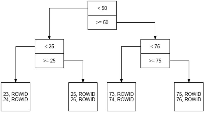
Figure 7-1. A balanced tree
What Indexes to Create?
Which indexes to create is a question that is not easily answered. The temptation is to create too many, but it is equally easy to forget to create any. Oracle will do the best it can with the available indexes, and powerful modern hardware can sometimes compensate for the lack of appropriate indexes. A commonly used rule is to create an index for every column that is restricted in a query. This may be too many, because the query optimizer bases the decision to use an index on the available statistical information about the table, and some indexes may never be used. Also, as I explained earlier, indexes must be modified whenever the data is modified; and, therefore, indexes can slow down the database. However, there are some situations where indexes are not optional:
- Unique indexes are required to efficiently enforce the requirement of uniqueness; for example, no two employees can share a Social Security number. This is particularly true of any column or combination of columns designated as a primary key.
- Indexes should always be created on foreign keys. A foreign key is a column or set of columns that is required to map to the primary key of another table. Full table scans and table-level locks can result if a foreign key is not indexed. In Expert One-On-One Oracle, Tom Kyte says: “I sometimes wish I had a dollar for every time I was able to solve the insolvable hanging issue by simply running the query to detect un-indexed foreign keys and suggesting that we index the one causing the problem—I would be very rich.” Tom provides the script in the book—it can also be found at http://tkyte.blogspot.com/2009/10/httpasktomoraclecomtkyteunindex.html.
Oracle Database provides several “advisors” that can generate recommendations for improving the performance of SQL queries. Listing 7-1 provides an example of how you can use the QUICK_TUNE procedure to analyze an SQL statement and determine whether additional indexes would improve performance. In this case, the QUICK_TUNE procedure recommends that a function-based index be created and even provides the necessary SQL commands to do so; you can replace the system-generated name for the index with a more meaningful name. Note that you need a license for the Tuning Pack in order to use the QUICK_TUNE procedure.
Index-Organized Tables
Ordinary Oracle tables are often referred to as heaps because the data they contain is not sorted in any way; separate structures—indexes—are needed in order to identify the records of interest efficiently. The index-organized table (IOT) is a single structure that unites a table and an index for its primary key. No separate index for the primary key is necessary, because the table itself is structured exactly as if it were an index for the primary key; all the non-key data is stored on the leaf blocks together with the key data. Indexes for other columns can be created in precisely the same way as indexes on ordinary tables.
Index-organized tables have a number of advantages. The union of table and primary key index in a single structure results in increased efficiency of retrieval operations. Certain maintenance operations (such as the MOVE operation) can be performed on them without invalidating all the indexes. Finally, index-organized tables can offer dramatic performance improvements if the primary key is composed of multiple data items and the leading item partitions the data in a natural way: for example, the store name in a table that contains sales data. The performance improvement comes from the physical clustering of related data that naturally results, the increased likelihood of finding the required data in the buffer cache, and the consequent reduction in disk activity.
Advanced Topics
An advanced type of index known as the bitmap index uses a single bit (0 or 1) to represent each row. A bitmap is generated for each distinct value contained in the indexed column.
If the indexed column contains ever-increasing values, Oracle attempts to insert the index information into the same leaf block each time. This dramatically increases the frequency of splitting and balancing operations. The solution is to create a reverse key index.
Partitioning
Because Oracle tables are stored as heaps, with no discernible internal organization, new rows of data are simply appended to the end of the table or anywhere else in the table there happens to be room. The strategy of using indexes to find the required rows of data quickly works well up to a point. But it begins to reveal its limitations as the amount of data and the number of users approach the levels seen in modern data warehouses and in online stores such as Amazon.com.
To understand the problem with heaps, imagine a history book containing facts like the following: “The Declaration of Independence was adopted by the Second Continental Congress on July 4, 1776.” Suppose that these facts are not naturally organized into separate chapters for, say, individual countries, but are randomly scattered throughout the book. You can still use the alphabetical index at the back of the book to discover facts about the United States relatively easily; but each time you retrieve a fact, you may have to visit a different page. This would obviously not be an efficient process.
A page of a book is analogous to a data block on a storage disk, and a chapter of related information in a book is analogous to an Oracle partition. Partitions divide data tables into separate storage pools; rows of data can be allocated to each storage pool using some criterion. Suppose you have a very large table of credit-card transactions, and they are randomly stored throughout the table without regard to date. To process the transactions completed in the last month, Oracle must retrieve more blocks of data from the storage disks than if transactions were stored with regard to date. The solution is to create a separate partition for each month. If a query spans partitions, Oracle need only visit the appropriate partitions; this is called partition pruning.
Oracle provides several methods of partitioning large tables, including list partitioning, range partitioning, and interval partitioning. The partitions can themselves be subpartitioned. Indexes can also be partitioned, and it makes a lot of sense to do so.
![]() Tip Partitioning is a separately licensed, extra-cost option and must be purchased together with Oracle Enterprise Edition; it cannot be used with Oracle Standard Edition or with Oracle Express Edition.
Tip Partitioning is a separately licensed, extra-cost option and must be purchased together with Oracle Enterprise Edition; it cannot be used with Oracle Standard Edition or with Oracle Express Edition.
Advantages of Partitioning
I have already alluded to the fact that partitioning may improve performance of SQL queries by reducing the number of data blocks that have to be retrieved from the storage disks, but this is not the only advantage. Here are some others:
- A join operation on two tables that are partitioned in the same manner can be parallelized. That is, Oracle can perform simultaneous join operations, each one joining a partition of one table to the related partition in the other table; the results are pooled. This technique is suitable when you are dealing with large data warehouses; it requires more computing power but can reduce the time required to process an SQL query.
- Partitions make it particularly easy to purge unneeded data. Dropping a partition can be a painless operation; deleting large numbers of records from an unpartitioned table is a resource-intensive operation.
- Making a backup copy of a large data warehouse is a time-consuming and resource-intensive operation. If the data in an old partition does not need to be modified and the partition is located in a dedicated tablespace, the tablespace can be put into read-only mode and one last backup copy of the tablespace can be created for archival purposes. From that point onward, the tablespace need not be included in backup copies.
- If an old partition cannot be removed from the database, an alternative is to move it to slower and cheaper storage. The faster and more expensive storage can be reserved for more current and frequently queried data.
- Maintenance operations can be performed on individual partitions without affecting the availability of the rest of the data in the rest of the table. For example, old partitions can be moved to cheaper storage without impacting the availability of the data in the rest of the table.
List Partitioning
In this form of partition, the refinancing criterion for each partition is a list of values. Consider a retail chain that has stores in three states. You might store sales data in a table created in the manner illustrated in Listing 7-2.
Range Partitioning
In this form of partition, the refinancing criterion for each partition is a range of values. In the case described in the previous section, you might alternatively store sales data in a table created in the manner illustrated in Listing 7-3.
Interval Partitioning
One difficulty with partitioning by monotonically increasing data items such as dates is that new partitions have to be periodically added to the table; this can be accomplished using the ADD PARTITION clause of the ALTER TABLE command. Interval partitioning eliminates this difficulty by having Oracle automatically create new partitions as necessary. The example in the previous section can be rewritten as illustrated in Listing 7-4. Only one partition called olddata is initially created. New partitions are automatically created by Oracle as necessary when data is inserted into the table.
Hash Partitioning
Hash partitioning was useful before large RAID arrays became commonplace; it can be used to stripe data across multiple disks in order to prevent the reading and writing speed of a single disk from becoming a performance bottleneck in OLTP and other environments requiring very high levels of throughput. A hashing function (randomizing function) is applied to the data item used as the partitioning criterion in order to allocate new rows to partitions randomly. Listing 7-5 illustrates the use of this technique; the data is spread over four tablespaces, which are presumably located on separate disk drives.
Reference Partitioning
Sometimes it makes sense to partition two or more tables using the same data item as the partitioning criterion even though the tables do not share the data item. As an example, consider the Orders and LineItems tables in Listing 7-6. The two tables are linked by the purchase order number. It makes sense to partition the Orders table using the OrderDate data item. It would also make sense to partition the LineItems table using the same data item as the criterion even though it is not part of the table. This can be accomplished using referential partitioning. Any number of tables can thus be partitioned using a common partitioning criterion that appears in only one of the tables.
Composite Partitioning
Oracle offers the ability to further divide a partition into subpartitions using different criteria; this can make sense if a table is very large. In Listing 7-7, you first create one partition for each month (using the interval partitioning method) and then create subpartitions for each state.
Local and Global Indexes
Partitioning a table does not eliminate the need for any of its indexes. However, you must make a design choice for each index; indexes on partitioned tables can be either local or global. A local index is itself partitioned in exactly the same way as its table; you only need to specify the LOCAL clause when creating the index to automatically create the necessary partitions for the use of the index. Local indexes are most suitable when the query specifies the partitioning criterion. They also promote partition independence; that is, they preserve your ability to perform maintenance operations on a partition without impacting the availability of the rest of the data in the table. Global indexes are most suitable when the query does not specify the partitioning criterion. A global index may or may not be partitioned and can even have a different partition scheme than its table.
Partitioned Views
The partitioning capabilities you have just learned about were introduced in Oracle 8 and have their roots in much older capabilities called partition views or—more properly—partitioned views. Partition views are simply views formed by the UNION ALL of separate tables, each of which contains a range of data values. The following paragraph is found in the Oracle7 Tuning guide:
You can avoid downtime with very large or mission-critical tables by using partition views. You create a partition view by dividing a large table into multiple physical tables using partitioning criteria. Then create a UNION-ALL view of the partitions to make the partitioning transparent for queries. Queries that use a key range to select from a partition view retrieve only the partitions that fall within that range. In this way partition views offer significant improvements in availability, administration and table scan performance.
Partitioned views do not offer all the features of the partitioning feature, but the prime reason to consider them is that—unlike regular partitions—they can be used with Standard Edition.
Consider the Sales fact table from the SH sample schema, one of the sample schemas provided by Oracle. The Sales table has five dimensions—product, customer, time, channel, and promotion—and two measurements—quantity sold and amount sold. It is partitioned into 28 partitions using the time dimension. The five dimensions are linked by foreign key constraints to the dimension tables, and there is a bitmap index on each of the dimensions. Here is the definition of the table:
CREATE TABLE SALES
(
  -- dimensions
  PROD_ID NUMBER NOT NULL,
  CUST_ID NUMBER NOT NULL,
  TIME_ID DATE NOT ENABLE,
  CHANNEL_ID NUMBER NOT NULL,
  PROMO_ID NUMBER NOT NULL,
  -- measurements
  QUANTITY_SOLD NUMBER(10,2) NOT NULL,
  AMOUNT_SOLD NUMBER(10,2) NOT NULL,
  -- constraints
  CONSTRAINT SALES_CHANNEL_FK FOREIGN KEY (CHANNEL_ID) REFERENCES SH.CHANNELS (CHANNEL_ID),
  CONSTRAINT SALES_TIME_FK FOREIGN KEY (TIME_ID) REFERENCES SH.TIMES (TIME_ID),
  CONSTRAINT SALES_PRODUCT_FK FOREIGN KEY (PROD_ID) REFERENCES SH.PRODUCTS (PROD_ID),
  CONSTRAINT SALES_CUSTOMER_FK FOREIGN KEY (CUST_ID) REFERENCES SH.CUSTOMERS (CUST_ID),
  CONSTRAINT SALES_PROMO_FK FOREIGN KEY (PROMO_ID) REFERENCES SH.PROMOTIONS (PROMO_ID)
)
-- partition by the time dimension
PARTITION BY RANGE (TIME_ID)
(
  -- annual partitions for 1995 and 1996
  PARTITION SALES_1995 VALUES LESS THAN ’1996-01-01’,
  PARTITION SALES_1996 VALUES LESS THAN ’1997-01-01’,
  -- semi-annual partitions for 1997
  PARTITION SALES_H1_1997 VALUES LESS THAN ’1997-07-01’,
  PARTITION SALES_H2_1997 VALUES LESS THAN ’1998-01-01’,
  -- quarterly partitions for 1998
  PARTITION SALES_Q1_1998 VALUES LESS THAN ’1998-04-01’,
  PARTITION SALES_Q2_1998 VALUES LESS THAN ’1998-07-01’,
  PARTITION SALES_Q3_1998 VALUES LESS THAN ’1998-10-01’,
  PARTITION SALES_Q4_1998 VALUES LESS THAN ’1999-01-01’,
  … intervening sections for 1999, 2000, 2001, and 2002 not shown
  -- quarterly partitions for 2003
  PARTITION SALES_Q1_2003 VALUES LESS THAN ’2003-04-01’,
  PARTITION SALES_Q2_2003 VALUES LESS THAN ’2003-07-01’,
  PARTITION SALES_Q3_2003 VALUES LESS THAN ’2003-10-01’,
  PARTITION SALES_Q4_2003 VALUES LESS THAN ’2004-01-01’
);
And here are the definitions of the five indexes on each partition. The keyword LOCAL means the indexes are partitioned in the same manner as the table. In other words, each partition has a local index:
CREATE BITMAP INDEX SALES_CHANNEL_BIX ON SALES (CHANNEL_ID) LOCAL;
CREATE BITMAP INDEX SALES_CUST_BIX ON SALES (CUST_ID) LOCAL;
CREATE BITMAP INDEX SALES_PROD_BIX ON SALES (PROD_ID) LOCAL;
CREATE BITMAP INDEX SALES_PROMO_BIX ON SALES (PROMO_ID) LOCAL;
CREATE BITMAP INDEX SALES_TIME_BIX ON SALES (TIME_ID) LOCAL;
Let’s work on recasting the Sales table into a partition view composed of 28 separate tables with the same names as the partitions of the original table, each with its own indexes. Although this may seem like an unnecessary proliferation of tables and indexes, remember that table and index partitions are also independent, have explicitly assigned storage, and can be independently maintained. Here are the table-creation statements for four quarters of data:
CREATE TABLE SALES_Q1_2003 AS
  SELECT * FROM sales PARTITION (SALES_Q1_2003) NOLOGGING;

CREATE TABLE SALES_Q2_2003 AS
  SELECT * FROM sales PARTITION (SALES_Q2_2003) NOLOGGING;

CREATE TABLE SALES_Q3_2003 AS
  SELECT * FROM sales PARTITION (SALES_Q3_2003) NOLOGGING;

CREATE TABLE SALES_Q4_2003 AS
  SELECT * FROM sales PARTITION (SALES_Q4_2003) NOLOGGING;
Next, let’s create check constraints on the time dimension for each of the 28 tables. These check constraints are critical to the success of the partition view; you need some way to ensure that data is not inserted into the wrong table. Here are some examples:
-- the oldest table is only bounded on one side and may contain data from prior years
ALTER TABLE SALES_1995 ADD CONSTRAINT SALES_1995_C1 CHECK
 (time_id < ’1996-01-01’);

-- tables other than the SALES_1995 table are bounded on both sides
ALTER TABLE SALES_Q1_1998 ADD CONSTRAINT SALES_Q1_1998_C1 check
  (time_id >= ’1998-01-01’ AND time_id < ’1998-04-01’);

ALTER TABLE SALES_Q1_1998 ADD CONSTRAINT SALES_Q2_1998_C1 check
  (time_id >= ’1998-04-01’ AND time_id < ’1998-07-01’);

ALTER TABLE SALES_Q1_1998 ADD CONSTRAINT SALES_Q3_1998_C1 check
  (time_id >= ’1998-07-01’ AND time_id < ’1998-10-01’);

ALTER TABLE SALES_Q1_1998 ADD CONSTRAINT SALES_Q4_1998_C1 check
  (time_id >= ’1998-10-01’ AND time_id < ’1999-01-01’);
You need to create bitmap indexes on the individual tables that make up the partition views. Each of the 28 partitions has 5 bitmap indexes, for a total of 140 indexes:
CREATE BITMAP INDEX SALES_Q1_1998_SALES_CHAN_BIX ON SALES_Q1_1998(channel_id);
CREATE BITMAP INDEX SALES_Q1_1998_SALES_CUST_BIX ON SALES_Q1_1998(cust_id);
CREATE BITMAP INDEX SALES_Q1_1998_SALES_PROD_BIX ON SALES_Q1_1998(prod_id);
CREATE BITMAP INDEX SALES_Q1_1998_SALES_PROM_BIX ON SALES_Q1_1998(promo_id);
You also need to add foreign key constraints on the individual partitions. Each of the 28 partitions has 5 constraints, for a total of 140 constraints:
ALTER TABLE SALES_Q1_1998 ADD CONSTRAINT SALES_Q1_1998_CHAN_FK
  FOREIGN KEY (channel_id) REFERENCES channels;

ALTER TABLE SALES_Q1_1998 ADD CONSTRAINT SALES_Q1_1998_CUST_FK
  FOREIGN KEY (cust_id) REFERENCES customers;

ALTER TABLE SALES_Q1_1998 ADD CONSTRAINT
  SALES_Q1_1998_PROD_FK FOREIGN KEY (prod_id) REFERENCES products;

ALTER TABLE SALES_Q1_1998 ADD CONSTRAINT SALES_Q1_1998_PROM_FK
  FOREIGN KEY (promo_id) REFERENCES promotions;

ALTER TABLE SALES_Q1_1998 ADD CONSTRAINT SALES_Q1_1998_TIME_FK
  FOREIGN KEY (time_id) REFERENCES times;
You’re now ready to create the partition view; let’s call it sales2. Notice that the partition view is a UNION ALL of 28 SELECT * sections. Note that each section includes the restriction on the time dimension. This gives the optimizer the information it needs to perform partition pruning during query execution:
CREATE OR REPLACE VIEW sales2 AS
SELECT * FROM SALES_1995 WHERE time_id<’1996-01-01’
UNION ALL SELECT * FROM SALES_1996 WHERE time_id >= ’1996-01-01’ AND time_id<’1997-01-01’
UNION ALL SELECT * FROM SALES_H1_1997 WHERE time_id>=’1997-01-01’ AND time_id<’1997-07-01’
UNION ALL SELECT * FROM SALES_H2_1997 WHERE time_id>=’1997-07-01’ AND time_id<’1998-01-01’
UNION ALL SELECT * FROM SALES_Q1_1998 WHERE time_id>=’1998-01-01’ AND time_id<’1998-04-01’
UNION ALL SELECT * FROM SALES_Q2_1998 WHERE time_id>=’1998-04-01’ AND time_id<’1998-07-01’
UNION ALL SELECT * FROM SALES_Q3_1998 WHERE time_id>=’1998-07-01’ AND time_id<’1998-10-01’
UNION ALL SELECT * FROM SALES_Q4_1998 WHERE time_id>=’1998-10-01’ AND time_id<’1999-01-01’
… intervening lines not shown
UNION ALL SELECT * FROM SALES_Q1_2003 WHERE time_id>=’2003-01-01’ AND time_id<’2003-04-01’
UNION ALL SELECT * FROM SALES_Q2_2003 WHERE time_id>=’2003-04-01’ AND time_id<’2003-07-01’
UNION ALL SELECT * FROM SALES_Q3_2003 WHERE time_id>=’2003-07-01’ AND time_id<’2003-10-01’
UNION ALL SELECT * FROM SALES_Q4_2003 WHERE time_id>=’2003-10-01’ AND time_id<’2004-01-01’;
Denormalization and Materialized Views
Denormalization is a technique that is used to improve the efficiency of join operations. Consider the Orders and LineItems tables from the order-management database described in Oracle Database 11g Java Developer’s Guide. To avoid having to join these tables, you can replace them with a table that contains all the data items from both tables. This eliminates the need to join the two tables frequently, but it introduces its own set of problems. Data items such as ToStreet, ToCity, ToState, and ToZip must now be duplicated if there is more than one line in an order. And if any of these data items needs to be changed, multiple data rows must be updated. The duplication of data thus creates the possibility that mistakes will be made.
You can use materialized views to avoid the problems created by denormalization. Instead of replacing the Orders and LineItems tables with a denormalized table, you could prejoin the tables and store the results in a structure called a materialized view, as illustrated in Listing 7-8.
The data items from the Orders tables are still duplicated, but the responsibility for accurate modifications to the materialized view rests with Oracle, which modifies the data in the materialized view whenever the data in the underlying tables is modified. For example, if the ToStreet data item of an order is modified, Oracle modifies all occurrences in the materialized view. Note that materialized views need to be indexed just like regular tables and can be partitioned if appropriate.
Materialized views can be directly referenced in SQL queries, but the same level of performance enhancement is obtained even if they are not directly referenced. Notice the ENABLE QUERY REWRITE clause in the command used to create the Orders_LineItems materialized view: the optimizer silently rewrites queries and incorporates materialized views if possible.
Clusters
In his book Effective Oracle by Design (Osborne Oracle Press, 2003), Tom Kyte quotes Steve Adams as saying, “If a schema has no IOTs or clusters, that is a good indication that no thought has been given to the matter of optimizing data access.” Although most people wouldn’t agree with Steve’s conclusion, it is true that most databases use only the simplest of table and index organizations—heap and b-tree, respectively—and don’t exploit the wealth of data-access mechanisms provided by Oracle.
Clusters improve the efficiency of the memory cache (and consequently of join operations) because data from related tables can be stored in the same data blocks. Oracle itself uses the cluster mechanism to access some of the most important tables in the data dictionary; the C_OBJ# cluster contains 17 tables including TAB$ (tables), COL$ (columns of tables), IND$ (indexes) and ICOL$ (columns of indexes). Oracle also uses the cluster mechanism in its spectacular TPC benchmarks; in one benchmark that was submitted in February 2007, an Oracle database achieved a throughput of more than 4 million transactions per minute.
Hash clusters provide quick access without the need for an index (if the value of the clustering key is specified in the SQL query). Listing 7-9 first preallocates space for a cluster called Orders_LineItems with 10,000 hash buckets, each of size 2KB. When inserting a new data row in the cluster, Oracle uses a hash function to convert the cluster key (PONo in this case) into the address of a random hash bucket where it will store the row. When the row is retrieved later, all Oracle has to do is use the same hash function to locate the row.
You use the cluster to store rows from the Orders table as well as the LineItems table, which means related rows from the LineItems table are stored in the same storage bucket along with the corresponding row from the Orders table. SQL queries that join the two tables and specify what value the PONo data item should have can now be expected to be very efficient.
Summary
Performance considerations can remain at the forefront throughout the life of a database. For example, new queries may be introduced at any time. Database administrators must therefore understand the mechanisms that can be used to improve performance. This chapter provided an overview of these mechanisms. Here is a short summary of the concepts touched on in this chapter:
- The first stage in database design is called logical database design or data modeling and is conducted without reference to any specific database technology such as Oracle or Microsoft SQL Server.
- Physical database design follows logical database design. First, the logical model is mapped to the proprietary data types, language elements, and mechanisms provided by the chosen database technology. Next, security requirements are implemented using the various mechanisms provided by the technology, such as views. Finally, you consider performance—the ability of the database engine to handle work requests efficiently.
- The three broad categories of performance mechanisms are indexes to quickly find data, partitions and clusters to organize data, and materialized views and denormalized tables to perform expensive operations like joins ahead of time.
- An Oracle index is analogous to the index of words at the back of this book and allows Oracle to quickly locate a row of data that satisfies the restrictions of a query. However, indexes don’t help much if a large percentage of rows in the table satisfy the restrictions of the query.
- A proliferation of indexes can negatively affect efficiency because Oracle must update all the relevant indexes whenever the data in a table is modified.
- Oracle indexes are structured for ease of use. The typical Oracle index is a balanced tree or b-tree.
- SQL Access Advisor can analyze an SQL query and determine whether an additional index would improve performance.
- An index-organized table (IOT) is a single structure that unites a table and an index for its primary key.
- Partitions divide data tables into separate storage pools. Rows of data can be allocated to each storage pool using some criterion. The partitioning methods provided by Oracle include list partitioning, range partitioning, interval partitioning, reference partitioning, hash partitioning, and composite partitioning.
- Indexes on partitioned tables can be local or global. A local index is itself partitioned in the same way as its table. Local indexes are most suitable when the query specifies the partitioning criterion; they also promote partition independence. Global indexes are most suitable when the query does not specify the partitioning criterion. A global index may or may not be partitioned and can even have a different partition scheme than its table.
- Partitioned views offer some of the advantages of the partitioning feature—partition pruning in particular. They can be used even with Standard Edition.
- Denormalized tables and materialized views can be used to improve the efficiency of join operations. Oracle automatically modifies the data in a materialized view whenever the data in the underlying tables is modified. The optimizer silently rewrites queries and incorporates materialized vies if possible. Materialized views can also be used to aggregate information or to synchronize satellite databases.
- Hash clusters provide quick access without the need for an index (if the value of the clustering key is specified in the SQL query). They improve the efficiency of the memory cache (and consequently of join operations) because data from related tables can be stored in the same data blocks.