Simple Aggregates

To get started with window functions we will use them to write alternate queries for some of the simple aggregates we encountered in Chapter 8. Let’s reconsider a simple aggregate query to count and average members’ handicaps:

SELECT COUNT(Handicap) AS Count, AVG(Handicap * 1.0)as Average
FROM Member;

The output for the query is shown in Figure 9-1.

Figure 9-1. Output for simple count and average of handicaps

With simple aggregates the only attributes allowed in the SELECT clause are the aggregate and those attributes included in a GROUP BY clause. This means we no longer have access to the individual handicaps contributing to the results.

Window functions allow us to retrieve the underlying data along with the aggregates. The keyword for window functions is OVER(); they are also sometimes referred to as over functions.

Here is a query similar to the preceding one using the OVER() function :

SELECT MemberID, LastName, FirstName, Handicap,
     COUNT(Handicap) OVER() AS Count,
     AVG(Handicap * 1.0) OVER() as Average
FROM Member;

Unlike the simple COUNT() function, with the OVER() function we are able to include additional fields in the SELECT clause. In the preceding query we have included four fields of detailed data about each member along with the two aggregates (which are indented on new lines to make them easier to read). The aggregates are just the same as the simple aggregates but include the OVER() function.

Part of the output of the preceding query is shown in Figure 9-2. The count and average of the handicaps appear with the detailed data for each member.

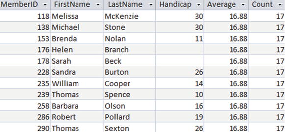
Figure 9-2. Output when using OVER() to count and average handicaps

While it doesn’t seem particularly useful in the example in Figure 9-2 to have the aggregates returned for every row, it opens the door to some new queries. We are now able to easily compare each individual’s handicap with the average, something that was not at all simple without window functions. On the third line of the following query we subtract the average of the handicap from the handicap for each member and include that in the SELECT clause:

SELECT MemberID, LastName, FirstName, Handicap,
     AVG(Handicap * 1.0) OVER() AS Average,
     Handicap - AVG(Handicap *1.0) OVER() AS Difference
FROM Member;

The result is displayed in Figure 9-3.

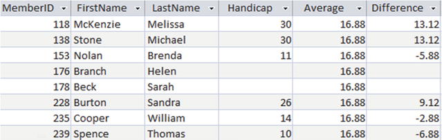
Figure 9-3. Window functions allow us to compare aggregates with detail values

Partitions

The OVER() function can also be used to produce queries that are similar to the GROUP BY queries we looked at in the previous chapter. The key phrase we need here is PARTITION BY. Let’s try some different counts on rows in the Entry table. If we use just the function OVER() with our COUNT(*) function, we will count all the rows, whereas if we use OVER(PARTITION BY TourID) it will count the rows for each different value of TourID.

The real power of partitioning is that, unlike the GROUP BY clause for simple aggregates, it is possible to have several different partitions in a single query. This is best explained by an example. The following query includes three different counts:

SELECT MemberID, TourID, Year,
COUNT(*) OVER() as CountAll,
COUNT(*) OVER(PARTITION BY TourID) AS CountTour,
COUNT(*) OVER(PARTITION BY TourID, Year) AS CountTourYear
FROM Entry;

The output is shown in Figure 9-4.

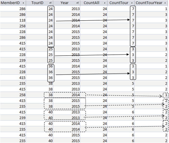
Figure 9-4. Using different partitions in a single query

In Figure 9-4 the column CountAll displays the result of COUNT(*) OVER(), which counts every row in the Entry table (24).

The column CountTouris the result of COUNT(*) OVER(TourID), which partitions (or groups) the rows with the same value of TourID and then counts them. The top three sets of solid boxes in Figure 9-4 show the rows contributing to CountTour for TourID of 24, 25, and 36.

The column CountTourYearis the result of COUNT(*) OVER(TourID, Year) and partitions all the rows with the same values for TourID and Year. The set of dashed boxes toward the bottom of Figure 9-4 shows examples of how these counts are evaluated.

Order By Clause

The OVER() function can include an ORDER BY clause . This specifies an order for the rows to be visited when the aggregates are evaluated. Having an order for the rows provides a mechanism for carrying out running totals and ranking operations.

Cumulative Aggregates

If an ORDER BY clause is included in the OVER() function then, by default, the aggregate is carried out from the beginning of the partition to the current row (but see below for a more precise definition).

Have a look at the following query:

SELECT MemberID, TourID, Year,
COUNT(*) OVER(ORDER BY Year) AS Cumulative
FROM Entry;

In the Entry table we have several rows with the same value of Year (as you can see in Figure 9-5). As far as the ordering goes, these rows are equivalent, so if one of them is included in a count then we should include them all. I’ll now correct the definition of what rows are included in the aggregate.

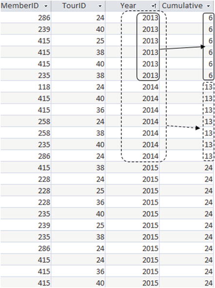
Figure 9-5. Using ORDER BY to produce a cumulative count for each year

If an ORDER BY clause is included in the OVER() function then, by default, the aggregate is carried out from the beginning of the partition to the current row, and includes any following rows with the same value of the ordering expression.

The output in Figure 9-5 illustrates what this means.

In Figure 9-5 the rows are ordered by Year. Let’s see how this cumulative counting works for the first few rows. For the first row, if we count from the beginning of the table we have 1 row. However, the next five rows have the same value for our ordering expression Year, so we include them in the count, giving us a total of 6.

Now let’s move down to the first row for member 258. Counting from the beginning of the table we have 10 rows, but the next 3 rows have the same value of Year. This makes a total of 13.

Essentially, we have a cumulative count of entries for each year. We have 6 entries in the first year (solid boxes), and for the second year we have an additional 7 entries to make 13 total (dashed boxes).

The SUM() function works in much the same way if there is an ORDER BY clause in the OVER() function to give us running totals.

Let’s say the club collects data on income from fundraising and tournaments in a table called Income. Figure 9-6 shows income for the first six months.

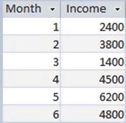
Figure 9-6. Income table

We can find a running total of the income by performing a SUM(Income) with an ORDER BY Month clause in the OVER() function, as in the following query:

SELECT Month, Income,
SUM(Income) OVER(ORDER BY Month) AS RunningTotal
FROM Income;

The income is summed from the beginning of the table to the current row (when ordered by the value of Month), as shown in Figure 9-7.

Figure 9-7. Running totals for monthly income ordered by month

Ranking

Yet another use for the ORDER BY clause is with the RANK() function . As an example we will rank the members of the club by their handicap. Have a look at the following query:

SELECT MemberID, Handicap,
RANK() OVER (ORDER BY Handicap) AS Rank
FROM Member
WHERE Handicap IS NOT NULL;

The ORDER BY clause in the OVER() function specifies the order of the rows when determining the rank—in this case the value of Handicap. Each time the value of Handicap changes, the rank becomes the row number in the partition (in this case the entire table ordered by Handicap).The rank then stays the same until the value of Handicap changes, as shown in Figure 9-8. (Some of the handicaps have been changed to illustrate the process more clearly. Rows with the same value of Handicap and therefore rank have been delineated.)

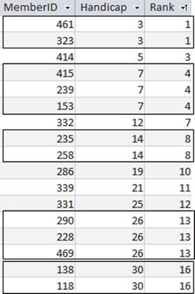
Figure 9-8. Result of the RANK() function ordered by handicap. Rows with the same value handicap have the same rank

The first row in Figure 9-8 has rank 1 (it is the first row!). The second row has the same value of the order expression (Handicap) as the previous row so it also has rank 1. In the next row the value of Handicap has changed so the rank becomes the row number (3).

Null values will be included in the ranking, which is why they have been explicitly excluded in the previous query. Without the WHERE clause the null values would have been included at the top of the ranking (or at the bottom if the order had been DESC).

Combining Ordering with Partitions

In the previous sections on ordering I didn’t include any partitions in the queries. Now that we (hopefully) understand the concept we can look at some more examples.

Let’s consider a more detailed Income table that has monthly amounts for each of three areas where the golf club carries out fundraising. The data for the first five months of the year is shown in Figure 9-9.

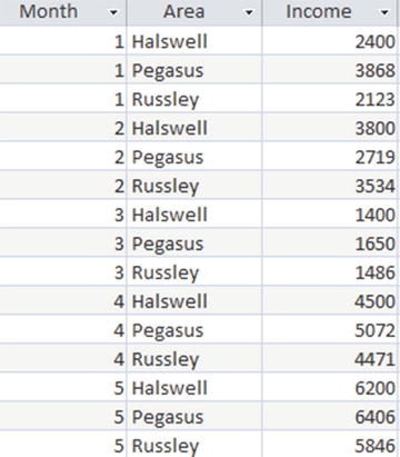
Figure 9-9. Income table including areas

We will build up some queries slowly.

First, we will just calculate the total income for the table. We could use a simple SUM() aggregate, but we will include an OVER() function so we can keep the detail in the output:

SELECT Month, Area, Income,
   SUM(Income) OVER() AS Total
FROM Income;

This will produce a table the same as in Figure 9-9 but with an additional column, Total, which will have the overall total for every row.

Now let’s change this to a running total. We do this by including an ORDER BY clause in the OVER() function. By default this calculates the total for the values from the beginning of the table to the current row and the next rows with the same value of Month. The query is:

SELECT Month, Area, Income,
   SUM(Income) OVER(ORDER BY MONTH) AS RunningTotal
FROM Income;

The incomes are summed from the top of the table to the current row including the following rows with the same value of Month (the attribute we are ordering by). Essentially, the output sums all the values for each month and then accumulates the totals month by month. The output is shown in Figure 9-10. The different months have been delineated.

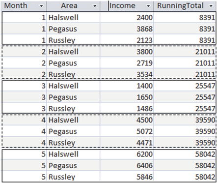
Figure 9-10. Running total when ordering by month

Now let’s look at the areas independently. This requires a PARTITION BY clause. Consider this query:

SELECT Month, Area, Income,
   SUM(Income) OVER(
      PARTITION By Area
      ORDER BY MONTH) AS AreaRunningTotal
FROM Income;

The PARTITION BY clause needs to come before the ORDER BY clause, which reflects what is happening. We first partition the data and then order within the partitions. The aggregate is calculated for rows from the beginning of the current partition to the current row. Figure 9-11 shows the output for just the first five months of the year. The three partitions have been delineated so it is easier to see what is happening.

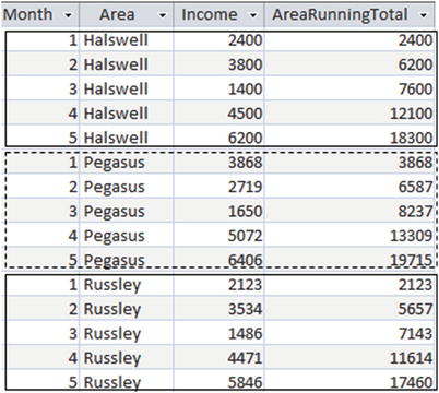
Figure 9-11. Running totals for income partitioned by area and ordered by month

Framing

The last feature of the window functions we will look at is the ability to further specify which rows are included in an aggregate. This is how the name window functions came about. They provide a window or frameonto the section of data we are interested in. The general form of the OVER() function has three clauses, as shown here:

OVER(
     [ <PARTITION BY clause> ]
     [ <ORDER BY clause> ]
     [ <ROWS clause> ]
     );

We have already looked at two of these clauses: The PARTITION BY clause allows us to group the data by some expression before aggregating. The ORDER BY clause allows us to determine the order in which the aggregate function traverses the rows within a partition and allows us to perform ranking and running totals. A ROWS clause allows us to narrow down the set of rows, relative to the current row, that are to be included in the aggregate.

By default, a query with an OVER(ORDER BY) clause calculates the aggregate of the values from the beginning of the current partition up to and including the current row. Let’s recap with a query that calculates a running average for each area:

SELECT Month, Area, Income,
AVG(Income) OVER (
     PARTITION BY AREA
     ORDER BY Month) AS AreaRunningAverage
FROM Income;

The output in Figure 9-12 is for just the Halswell area. The solid boxes show which rows are included in the average for the third row from the top. The dashed boxes show the rows contributing to the average for the third row from the bottom of the image. If there is no ROWS clause after an ORDER BY clause, then this is the default behaviour.

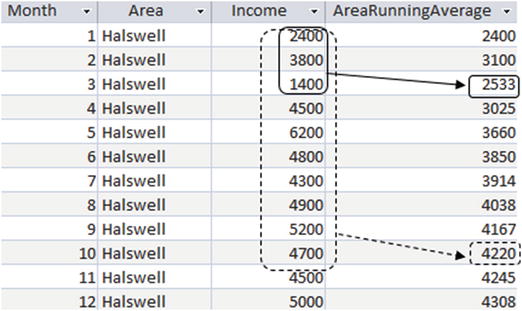
Figure 9-12. Running average for Income table

The syntax for the ROWS clause is:

 ROWS BETWEEN <start of frame> AND <end of frame>

Table 9-1 shows some expressions for specifying <start of frame> and/or <end of frame>. Remember that we always have to have an ORDER BY clause if we are using the ROWS clause.

Here is the previous query with the (default) window of required rows spelled out:

SELECT Month, Area, Income,
    AVG(Income) OVER(
       PARTITION BY AREA
       ORDER BY Month
       ROWS BETWEEN UNBOUNDED PRECEDING AND CURRENT ROW
    ) AS AreaRunningAverage
FROM Income;

The ROWS clause in the preceding query is the default if no ROWS clause is specified after an ORDER BY clause.

Now we can change which rows are to be included in the average. Say we would like to see rolling three-month averages. This means that for each month we take an average that includes the current month, the one preceding, and the one following. The following query shows how we can add another ROWS clause to the preceding query to see both the running average and the rolling three-month average:

SELECT Month, Area, Income,
    AVG(Income) OVER(
       PARTITION BY AREA
       ORDER BY Month
       ROWS BETWEEN UNBOUNDED PRECEDING AND CURRENT ROW
    ) AS AreaRunningAverage,
    AVG(Income) OVER(
       PARTITION BY AREA
       ORDER BY Month
       ROWS BETWEEN 1 PRECEDING AND 1 FOLLOWING
    ) AS Area3MonthAverage
FROM Income;

Figure 9-13 shows the output of this query. The boxes show which values are contributing to the averages on the rows for month 4 (solid boxes) and month 9 (dashed boxes).

Figure 9-13. Running averages and rolling three-month averages

The RunningAverage in the row for month 4 includes all the values from the beginning to month 4, and similarly the RunningAverage in the row for month 9 includes all the incomes up to and including month 9. The Rolling3MonthAverage in row 4 includes months 3 to 5 (one month preceding and one month following the current row). In row 9 the Rolling3MonthAverage averages months 8 to 10 (i.e., one month each side of month 9).

The different averages provide different information about the how the business is doing. The running average provides the average income to date for the year. The rolling three-month average gives a better idea of how the income is tracking at the moment. The later values in the rolling average column are higher than their running average counterparts because they are not including the lower values in the first few months.

Summary

Window functions provide an elegant way to carry out partitioning, running, and rolling aggregates and allowing both the detail and the aggregate to be available in the same query.

Here is a brief summary of the functionality covered in this chapter. I have used the word table in the descriptions but the functionality equally applies to the result of a query.