
Relational database theory is based on set theory.1 When we query a database we are essentially formulating a question to retrieve a subset containing the information we require. There are two approaches for retrieving a subset of data. Relational algebra is a description of the operations to perform on the data (in the body of the book we called this the process approach). Relational calculus describes conditions that the retrieved data must satisfy (we referred to this as the outcome approach). In this appendix we introduce the formal notation to formulate queries using relational algebra and calculus. This will allow you to think about queries from a different perspective. If you are interested in following up on the formal mathematics, There are more theoretical publications available.2 No new concepts are presented here that have not been discussed previously—it is just the notation that is different. The more formal notation allows queries to be expressed very concisely, and the underlying mathematics can be useful when dealing with complex situations. We will use the database described in Appendix 1 for the examples.
Introduction
As an example of how thinking of data as sets can help us, let’s consider a set that contains information about all the people on Earth. We can define a subset that contains all the men, another that contains all the golfers, another that contains people over 40, and another that contains Italians. These sets can all overlap, as shown in the diagram in Figure A2-1. This type of diagram is called a Venn diagram .
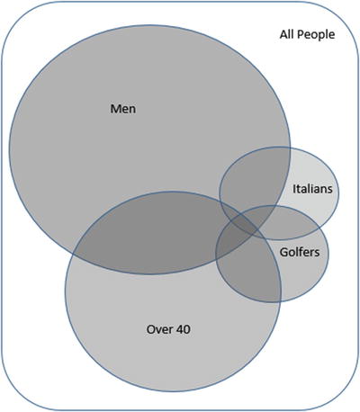
Figure A2-1. Venn diagram showing subsets of people
Figure A2-1 helps us visualize the sets that satisfy criteria such as Italian men over 40 who play golf (the area where all the circles overlap) or people who don’t play golf (everywhere in the large rectangle except the Golfers circle). These two areas are easy to describe; however, it is not always simple to define the subset we require. The area containing Italian golfers who are 40 or under takes a bit more effort to find, and it is difficult to describe without the diagram to help.
A database is only useful if you can accurately extract the appropriate subset of data when you need it. As the criteria become more complex and the number of tables increases, it can become difficult to keep everything in your head and correctly describe what you are trying to find. It is in these more complex situations that having a more formal and succinct notation can be very helpful.
Relations, Tuples, and Attributes
It is common to think of a database as a number of tables. A table (e.g., Person) will have a several columns. Each row in the table represents an individual person with the appropriate values for that person appearing in each column. More formally, a database is referred to as a set of relations, and each relation is a set of tuples. A tuple is a set of attribute values; for example, {Ali, Brown, 2/8/1967}.
A relation consists of a heading and a body. The heading is a description of the data that is contained in the relation. Part of that description is a set of attribute names; for example, {FirstName, LastName, Date_of_Birth}. In addition, each attribute has a domain, or set of allowed values. For example, Date_of_Birth must be a valid date. A domain can be a primitive type (e.g., integer, string) or a user-defined type (e.g., WeekDays = {Mon, Tue, Wed, Thu, Fri, Sat, Sun}). A database schema is the set of headings for all the relations plus any constraints that have been defined.
The body of the relation contains the data values. It consists of tuples containing values for each of the attributes.
Table A2-1 shows analogous terms for the two ways of describing a database.
Table A2-1. Comparative Terms
Relational Term | Database Term |
|---|---|
Database (set of relations) | Database |
Relation (set of tuples) | Table |
Tuple (set of attribute values) | Row |
Attribute name | Column Name |
Domain | Column datatype (primitive or user defined) |
The main differences between an (unkeyed) table and a relation or set of tuples are that there is no order to the tuples and each tuple must be unique.
Figure A2-2 shows how we can visualize a relation as a set of tuples.
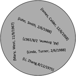
Figure A2-2. A relation is a set of tuples.
The traditional way of representing a set in a Venn diagram, as in Figure A2-1, reinforces the concept that there is no order to elements in a set. There is no first or next or previous element. The usual format for a table can imply that the rows have some sort of intrinsic order. When you query a database then, theoretically, the tuples returned have no guaranteed order unless you specify an order as part of the query. In practice, a simple query is likely to return rows in the same order each time it is repeated because under the hood the same operations will be carried out. However, with large tables, as the number of tuples changes the number and order of the operations may change to improve efficiency, or data that has been previously cached may be accessed first. These may affect the order in which tuples are returned.
As discussed in Chapter 1, having unique tuples in a relation is essential if we are going to be able to identify our data correctly. If, in the relation in Figure A2-2, we found we had another person called John Smith born on 2/6/1988 we would be in trouble, because we would not be able to distinguish the tuples for the two people. We need enough information stored about people so that they can be differentiated. The concept of a primary key (a set of attributes that must be unique for every tuple) ensures uniqueness.
Once we think of our data as sets of tuples then all the power of set operations is at our disposal.
SQL, Algebra, and Calculus
SQL is a language that is mostly based on relational calculus. Relational calculus describes the conditions the retrieved tuples must obey. In the following SQL query, the WHERE clause describes the resulting tuples:
SELECT LastName, FirstName, Handicap, PracticeNightFROM Member, TeamWHERE TeamName = Team AND Handicap < 15;
Although SQL is a calculus-based language, more and more keywords suggesting set operations from relational algebra have been included in the syntax over the years. In many cases this makes the queries easier to understand. The preceding query can also be written using the syntax associated with the relational algebra inner join operation, as follows:
SELECT LastName, FirstName, Handicap, PracticeNightFROM Member INNER JOIN Team ON TeamName = TeamWHERE Handicap < 15;
The preceding SQL appears to suggest that the join is carried out first and then those tuples with Handicap < 15 are retrieved. This is not the case in practice. SQL is simply a description of the resulting tuples and does not imply how the query will be carried out. The database’s query optimizer will determine how the tuples are retrieved, and a good optimizer would carry out the two queries in the same (most efficient) way.
In the remainder of this appendix we will look at a more formal notation for relational algebra and calculus. I will often provide an equivalent SQL expression and will choose one that is similar to the algebra or calculus depending on the section. The important thing to remember is that all SQL expressions are descriptions of the query output, and the way they are expressed does not necessarily determine the operations involved in retrieving the resulting data.
Relational Algebra: Specifying the Operations
With relational algebra, we describe queries by considering a sequence of operations or manipulations on the relations in the database. Some operations act on one relation (unary operations), while others are different ways of combining data from two relations (binary operations). Every time we perform an operation on one or more relations the result is another relation. This is a very powerful concept and means we can build up complicated queries in small steps by taking the result of one operation and applying another operation to it.
The relational algebra operations and the symbols commonly used to represent them are shown in Table A2-2.
Table A2-2. Relational Operators and Their Symbols
Operation | Symbol |
|---|---|
select | σ |
project | π |
Cartesian product |
|
union | ∪ |
difference | - |
inner join | ⋈ |
intersection | ∩ |
division | ÷ |
The operations are not completely independent. For example, later we will see that an inner join is defined as a Cartesian product followed by a select and a project. The first five operators in Table A2-2 can be used to define the final three, which is why SQL does not need to provide keywords representing division and intersection. However, it is convenient to be able to specify the equivalent SQL for an operation such as inner join because it occurs so frequently in database queries. We will now introduce a more formal notation for each of the operations and show how it can be used to specify queries.
Select
The
select operation
returns just those tuples from a relation that satisfy a particular condition involving the attributes. An example of using a select operation would be to retrieve all the senior members from our Member relation. The Greek letter sigma (σ) stands for the select operation, and the condition, MemberType = 'Senior', is specified in a subscript. The following expression shows the notation for using select to return senior members:
![]()
Each tuple in the relation Member is investigated, and if the tuple meets the condition it is included in the resulting relation. In table terms, the select operator retrieves a subset of the rows of the table. All of the attributes or columns are returned.
In SQL the WHERE clause contains the condition for the select operator and controls the tuples or rows that are returned. The SQL equivalent of the select operation ![]() is:
is:
SELECT *FROM Member mWHERE m.MemberType = 'Senior';
Note that the SELECT keyword in SQL has nothing directly to do with the relational algebra select operation. More about that in the next section.
Project
The
project operation
returns a relation where the attributes are a subset of the attributes of a relation. The project operator is denoted by π (pi), and the attributes are listed in a subscript. In table terms, project returns a subset of the columns of a table. The following statement would return the FirstName and LastName attributes from every tuple in the relation Member:
![]()
How many tuples or rows would you expect to be returned from the Member relation as a result of the operation πFirstName(Member)? The tuples consist of the single attribute FirstName. The Member relation has 20 tuples, but that includes two occurrences of William, two of Robert, and three of Thomas. Earlier I mentioned that the result of every operation results in another relation. The result of πFirstName(Member) must be a set of unique tuples. The duplicates will all be removed, leaving us with 16 unique names.
Think of the project operation as returning all the unique combinations of values for the specified attributes.
In SQL the attributes to be returned by the project operator are specified in the SELECT clause. I know this seems perverse, but remember that SQL syntax is based on relational calculus, not on algebra. The SQL equivalent of the project operation πFirstName, LastName(Member) is:
SELECT DISTINCT FirstName, LastNameFROM Member;
Combining Select and Project
Because the result of an algebra operation on a relation always results in another relation, we can apply the operations successively. The following expression first uses the select operation to find all the tuples for senior members (the inner parentheses) and then applies the project operation to return just the names:
![]()
Does the order of the operations make a difference? Consider the following expression where the order of the select and project operations is reversed:
![]()
The tuples resulting from the initial project operation (inner parentheses) have just the two attributes FirstName and LastName. The MemberType attribute is no longer in the tuples, so we cannot use it in the select condition. The algebra expression is not valid.
The SQL statement equivalent to our combined select and project operations is:
SELECT FirstName, LastName FROM MemberWHERE MemberType = 'Senior';
Because SQL is based on relational calculus rather than algebra, there is no concept of operations or order in the preceding statement. It is just a description of the tuples to be retrieved.
For more complex queries it is sometimes helpful to introduce intermediate relations so we can break up the query into smaller steps. For example, we might call the relation resulting from the select operation SenMemb, as in the following:
![]()
Now we can use the project operation on the newly named relation SenMemb to return the names:
![]()
In SQL we can use views to break down queries into simpler steps. A view can be thought of as instructions for creating a new temporary relation:
CREATE VIEW SenMemb ASSELECT * FROM MemberWHERE MemberType = 'Senior';
The view can then be used in other queries:
SELECT LastName, FirstNameFROM SenMemb;
Cartesian Product
The select and project operations are both unary operations, which means they act on a single relation. We will now look at binary operations, which act on two relations. The result of both unary and binary operations is a single relation.
A
Cartesian productis the most versatile binary operation because it can be applied to any two relations. The notation for a Cartesian product between two relations Member and Team is:
![]()
Each tuple in a Cartesian product will have a value for each attribute from the two contributing relations. The tuples in the resulting relation consist of every combination of tuples from the original relations. If one relation has N tuples and the other M, then the resulting relations will have N x M tuples. In table terms, the Cartesian product takes two tables of any shape and produces a table with a column for each column in the original tables and a row for every combination of the original rows. Figure A2-3 shows abbreviated Member and Team tables and their Cartesian product.
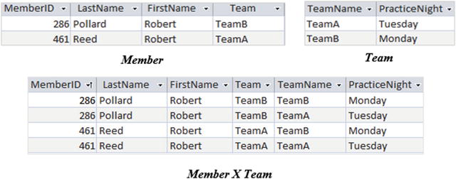
Figure A2-3. The Cartesian product of Member and Team
The SQL for a Cartesian product use the keyword CROSS JOIN, as in the following statement:
SELECT * FROM Member CROSS JOIN Team;Inner Join
In relational algebra an inner joinis defined as a Cartesian product followed by a select operation that compares the values of attributes from the two original relations. The attributes being compared must have the same domains.
Referring to the tables in Figure A2-3, we can specify a Cartesian product followed by a select that will return only those tuples where the value of Team is the same as the value of TeamName:
![]()
We can use the join operation to produce an equivalent expression. The join symbol ⋈ is used, and the select, or join, condition is expressed in a subscript as shown in the following expression:
![]()
The preceding expressions are equijoins where the select condition uses equality. This is the most common type of join. The more general case is a θ-join (theta-join) where the expression can include comparisons such as > and <. A natural join is one where the two relations each have one or more attributes with the same name. By default, the join condition will be equality on the values of the attribute with the same name, and one of those duplicate attributes will be removed from the final result with a project operation.
When we have expressions involving several operations we often have a choice as to the order in which the operations are applied. For example, if we want to retrieve the practice night for Mr. Pollard, we can either select Pollard from the Member relation before the join or afterward from the result of the join. These two options are shown here:
![]()
The tuples resulting from the preceding two expressions are the same; however, the method for obtaining them is quite different. The first will involve first creating a large relation that is the Cartesian product of Member and Team. In the second expression, we reduce the number of tuples in the Member relation to just those for Pollard and then construct a much smaller Cartesian product. Clearly the second expression will be more efficient.
SQL being based on calculus rather than algebra does not imply any ordering of operations. While the SQL statement that follows might suggest that the join is carried out first, it is just a statement describing the tuples to be retrieved:
SELECT *FROM Member INNER JOIN TEAM ON Team = TeamNameWHERE LastName = 'Pollard';
The query optimizer in a database system will determine an effective method for carrying out the query.
Union, Difference, and Intersection
Because a relation is defined as a set of tuples, the three binary set operations union (∪) , difference (−) , and intersection (∩) can be used for retrieving information. For relational algebra there is the additional constraint that the two relations involved in these operations must be union compatible. This means that the two relations must have the same number of attributes, and the corresponding attributes in each relation must be defined on the same domains.
For example, consider two relations with the following attributes:
Staff:{FamilyName, FirstName, Salary}Students:{LastName, Name, Address, Course}
The set operations will help us to retrieve the names of all the people (union), the names of those people who are both students and staff members (intersection), and those who are students but not staff and vice versa (difference). (This, of course, makes naïve assumptions about the uniqueness of names!)
We cannot compare tuples in the relations as they stand because they have different attributes. Staff and Student are not union compatible. One has a Salary while the other has an Address and a Course. However, the names can be compared, as they have the same domains (text) in each relation. We can retrieve just the names by applying a project operation to each of the original relations as follows:
![]()
![]()
Strictly speaking, for union compatibility the attributes should be identical (same name and domain). However, in practice just the domains need to be the same, and the order of the attributes determines what is compared. We can now apply any of the three set operations to the new union-compatible relations. For example:
![]()
The SQL expression is:
SELECT FamilyName, FirstName FROM StaffUNIONSELECT LastName, Name FROM Student;
We can continue applying operations to the results of our expressions. If taken slowly it is quite straightforward. For example, if we want to find the names and salaries of those staff who are also students we can build up a series of relational algebra operations starting with the initial relations. See the following:
1. Project out the names to get union-compatible relations.
2. Use the intersection operation to find those staff who are also students.
3. Join the result with the Staff relation so we have access to the Salary attribute.
4. Project the Names and Salary attributes.
You can see each of these operations in the following expression—just read the brackets from the inside to the outside:
![]()
Union, difference, and intersection are not independent. An intersection can be expressed in terms of two difference operations. Assuming StaffNames and StudentNames are two union-compatible relations, we have that:
![]()
Draw yourself a sequence of pictures to convince yourself of this.
Some versions of the SQL language do not implement the INTERSECT keyword because the query can be restated, as just seen, using EXCEPT (the SQL syntax for difference). The following SQL query uses the INTERSECT keyword:
SELECT * FROM StaffNamesINTERSECTSELECT * FROM StudentNames;
An equivalent query can be constructed using the EXCEPT keyword:
SELECT * FROM StaffNamesEXCEPT(SELECT * FROM StaffNamesEXCEPTSELECT * FROM StudentNames);
Division
Division is the last of the relational algebra operations we will consider. The easiest way to understand the division operation is with an example.
If we want to know which members of our club have entered every tournament, we need two pieces of information. We need information about the members and the tournaments they have entered, which we can get from the Entry table, and we also need a list of all the tournaments, which comes from the Tournament table.
In Figure A2-4, you can see how division works. It shows the MemberID and TourID attributes from the Entry relation, and the TourID attribute from the Tournament relation. The result of the division is the set of MemberID values that have a tuple in the Entry relation for every value TourID.
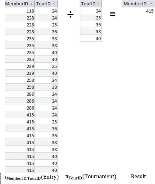
Figure A2-4. Using the division operator to find members who have entered all tournaments
The relational algebra expression for the division operation in Figure A2-4 is as follows:
![]()
There is no SQL keyword for the division operator. However, it is possible to express division in terms of other algebraic operations. It can be a bit daunting if presented in one step, so we will take it slowly.
First, find all the members who have entered a tournament and, by way of a Cartesian product, create tuples for each of those members paired with every tournament. We’ll call the resulting relation AllPairs:
![]()
Now we will remove from AllPairs the pairings that are in the Entry table by using a difference operation. If we project out the MemberID from the result we will have the IDs for members who are not associated with every tournament.
![]()
By removing these unmatched MemberIDs from the MemberIDs in the Entry relation we will arrive at the result we require:
![]()
We can use SQL views to express these same steps in a manageable way. First, create a view with all the pairs of members and tournaments:
CREATE VIEW AllPairs ASSELECT M.MemberID, T.TourID FROM(SELECT MemberID FROM Entry)MCROSS JOIN(SELECT TourID FROM Tournament)T;
Now create a view to find the unmatched pairs:
CREATE VIEW Unmatched ASSELECT * FROM AllPairsEXCEPTSELECT MemberID,TourIDFROM Entry;
Now use these two views to find the result of the division; i.e., the MemberID of members who have entered every tournament:
SELECT MemberID FROM EntryEXCEPTSELECT MemberID FROM Unmatched;
If you are brave you could try to combine all these steps into one SQL query; however, we will look at a more manageable way to express the equivalent query using relational calculus in the section on the universal quantifier later in this Appendix.
Relational Calculus: Specifying the Outcome
Relational algebra lets us specify a sequence of operations that eventually results in a set of tuples with the required information. Rather than specifying how to do the query, relational calculus describes what conditions the resulting data should satisfy. This section provides a very brief introduction to the notation for describing calculus queries without delving into the mathematics.
Simple Calculus Expressions
In informal language, a relational calculus description of a query has the following form:
I want the tuples that obey the following conditions....
More formally we can express the above as:
{ m | condition(m) }The part on the left of the bar | specifies the attributes in the tuples we want returned, while the part on the right (often referred to as the predicate) describes the criteria they must satisfy. m is called a tuple variable and condition(m) is a function that must be true for each of the tuples m returned. Strictly speaking, the preceding notation is called tuple calculus. Another equivalent notation, which we will not pursue here, is domain calculus.
The following expression means that each returned tuple m must be from the Member relation and must have ‘Senior’ as the value of the attribute MemberType:
{m | Member(m) AND m.MemberType = 'Senior'}We can further refine the expression to specify which attributes of the tuple m should be included in the result:
{m.LastName, m.FirstName | Member(m) AND m.MemberType = 'Senior'}Because SQL is based on relational calculus, the equivalent SQL statement is an almost direct translation of the calculus expression, as we see here:
SELECT m.LastName, m.FirstNameFROM Member mWHERE m.MemberType = 'Senior';
The part on the left of the bar | in the calculus expression becomes the SELECT clause, Member(m) becomes the FROM clause, and the rest of the expression makes up the WHERE clause. In SQL the m is can be referred to as a table alias, but it is useful to think of it as tuple variable as well.
Free and Bound Variables
The following calculus expression retrieves members’ names and the fee associated with their membership type. It is essentially an inner join between the Member and Type relations.
{m.LastName, m.FirstName, t.Fee | Member(m) Type(t) AND m.MemberType = t.Type}The tuple variables m and t are referred to as free variables. The conditions on the right of the expression cannot be evaluated until we give m and t values. It is usual to refer to the free variables as rangingover every tuple in their respective relations and then evaluating the conditions for each combination to see if it should be included in the result. In the body of the book I suggested thinking of the variables as being attached to fingers that move through their respective relations so we can determine if the condition (in this case m.MemberType = t.Type) evaluates to true. Free variables denote the tuples being returned and should always appear on the left of the bar.
Suppose we want to find the names of those members who have entered any tournament. In order to include a member in the result there has to be a tuple for that member in the Entry relation. The symbol ∃, meaning “there exists,” is used in the following calculus expression to return the names of those members where a tuple exists in the Entry relation with their MemberID:
{m.LastName, m.FirstName | Member(m) AND∃(e)(Entry(e) AND m.MemberID = e.MemberID)}
I’ve spread the expression out on different lines so that the conditions on the variable e are clear. The variable e is referred to as a bound variable. It does not appear on the left of the equation and is only used to determine whether the condition on the right side of the expression is true. The free variables (which always appear on the left side of the expression) are the ones for which we consider every possibility. In the preceding expression our free variable m is given the value of every tuple in the Member relation in turn. For each value of m we use the bound variable e to help determine if there is an appropriate tuple in the Entry relation.
Bound variables need to have what is called a quantifier, which explains how the variable will be used in calculating the condition statement. In this case we use the existential quantifier (∃), which requires us to find a single tuple in the associated relation that satisfies the condition. There is also a universal quantifier(∀) that requires every tuple in the associated relation to satisfy the condition. We will now look at examples of using these quantifiers and the equivalent SQL statements.
Existential Quantifier and SQL
An expression such as ∃(e)(Entry(e) AND (condition(e)) is true, if we can find a tuple e in the relation Entry that satisfies the specified condition. Let’s look at how this query can be represented in SQL:
{m.LastName, m.FirstName | Member(m) AND∃(e)(Entry(e) AND e.MemberID = m.MemberID)}
First, we’ll consider an SQL expression that follows the calculus as closely as possible by using an EXISTS clause:
SELECT m.LastName, m.FirstNameFROM Member mWHERE EXISTS (Select * FROM Entry e WHERE e.MemberID = m.MemberID);
As you can see, the SQL is almost a direct translation of the calculus statement. Equivalently, we can represent the existence requirement with a nested query and IN clause:
SELECT m.LastName, m.FirstNameFROM Member mWHERE m.MemberID IN (SELECT MemberID FROM Entry e);
Each of preceding SQL statements returns the correct result, but I’m sure you are thinking that they are a complicated way of getting there. The query to find members who have entered a tournament can be more simply expressed as a join between the two relations:
SELECT m.LastName, m.FirstNameFROM Member m, Entry eWHERE e.MemberID = m.MemberID;
The preceding SQL statement is not strictly equivalent to the first two. The latter one will return duplicate names, one for each of the tournaments the member has entered. If we look at the first two SQL queries, we see that they are checking each tuple in the Member table (just the once) and looking for a corresponding tuple in the Entry table. The final query considers all combinations of the tuples in Member and Entry and returns any that satisfy the condition (thereby returning the duplicates).
Even though we can remove the duplicates from the final SQL query by adding a DISTINCT keyword, it is considering a different set of tuples for inclusion in the result, and so is responding to a subtly different question than are the two earlier SQL statements. The relational calculus query is very precise, and it is that precision that can be helpful in some situations.
To find members who have not entered a tournament we simply replace ∃ with NOT ∃ (or ∄) in the query to find members who have entered a tournament:
{m.LastName, m.FirstName | Member(m) ANDNOT ∃(e)(Entry(e) AND m.MemberID = e.MemberID)}
The equivalent SQL statement simply requires the addition of the keyword NOT, as in the example here:
SELECT m.LastName, m.FirstNameFROM Member mWHERE NOT EXISTS (SELECT * FROM Entry eWHERE e.MemberID = m.MemberID);
Universal Quantifier and SQL
The universal quantifier∀ allows us to check that a condition holds for all tuples in some set. This is what we require in order for a query to find the names of members who have entered all tournaments. We have looked at this query many times! The relational calculus statement that follows is a straightforward way to express the query:
{m.LastName, m.FirstName | Member(m) AND∀(t)(Tournament(t)∃(e)(Entry(e) ANDe.MemberID = m.MemberIDAND e.TourID = t.TourID))}
The calculus statement should be interpreted as “Retrieve the LastName and FirstName for a particular tuple m in Member if for every tuple t in Tournament there exists a tuple e in Entry for the member m and the tournament t.”
You will recognize the outcome of this query as the equivalent of the relational algebra division operator. You will also remember that SQL does not have a keyword for division. Sadly, it doesn’t have a keyword for the universal quantifier either. Relational calculus can help us out here with the use of the following identity:
∀(t)(condition (t)) ≡ NOT ∃(t)(NOT condition(t))This statement means that if we say “for every tuple t a condition holds” then that is the same as saying “there is no tuple t for which the condition does not hold.” We can use this identity to recast our original calculus expression to the following:
{m.LastName, m.FirstName | Member(m) ANDNOT ∃(t)(Tournament(t)(NOT ∃(e)(Entry(e) AND e.MemberID = m.MemberIDAND e.TourID = t.TourID))}
Essentially, this says that there is no tuple t in Tournament for which there is not a corresponding tuple e in Entry. This translates quite easily to the SQL statement seen here:
SELECT m.LastName, m.FirstNameFROM Member mWHERE NOT EXISTS (SELECT * FROM Tournament tWHERE NOT EXISTS (SELECT * FROM Entry eWHERE e.MemberID = m.MemberIDAND e.TourID = t.TourID));
An Example
Let’s look at the algebra and calculus for a query that could be a little tricky. We want to find the names of the women who have never played in the Leeston tournament.
Algebra
First, we need to retrieve
all entries for the Leeston tournament by joining the Tournament and Entry tables and then using a select operation:
![]()
The words “have never” suggests we need a difference operator. So, we need to find the set of all women by using a select operation on the Member table, and then we need to remove the set of people who have played at Leeston. In order to use our difference operator we need to have union-compatible relations, so we will project just the MemberID from the two sets just described. The following expression will return the IDs of the women who have not entered the Leeston tournament:
![]()
Now we need to join NonLeestonLadies to the Member table so we have access to their names. We can retrieve the final set of names with:
![]()
We can now construct an SQL statement that reflects the algebra expression. In the following SQL the most indented rows represent the LeestonEntries, the next indentation represents the NonLeestonLadies (and has been given that alias), and the outer rows represent the final join and project:
SELECT m2.LastName, m2.FirstName FROM(SELECT m.MemberID FROM Member mWHERE m.Gender = 'F'EXCEPTSELECT e.MemberIDFROM entry e INNER JOIN tournament t ON e.tourID = t.tourIDWHERE t.TourName = 'Leeston')NonLeestonLadiesINNER JOIN Member m2 ON m2.MemberID = NonLeestonLadies.MemberID;
Calculus
Let’s approach the same query (the names of the women who have never played in the Leeston tournament) using calculus . I always need to visualize the tuple variables as fingers to get myself started. Figure A2-5 shows the relations that we will need for the query.
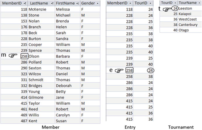
Figure A2-5. Tuple variables required for the query
We want to retrieve the names of women from the Member table, so we need to consider each tuple in turn. That means m will be our free variable. For each tuple m we need to check that the value of Gender is F and that there is no tuple e in the Entry table that has the same MemberID as m and also has TourID = 24 (the Leeston tournament). Figure A2-5 shows us that although Barbara Olson is a female, we will not include her as she has an entry for the Leeston tournament.
The following calculus expression will retrieve the names of members satisfying the conditions we have just described:
{m.LastName, m.FirstName | Member(m) AND m.Gender = 'F'NOT ∃(e)(Entry(e)(e.MemberID = m.MemberIDAND ∃(t)(t.TourID = e.TourIDAND t.Tourname = 'Leeston')}
The calculus expression translates directly to the following SQL statement:
SELECT m.LastName, m.FirstNameFROM Member mWHERE m.Gender = 'F'AND NOT EXISTS (SELECT *FROM Entry eWHERE e.MemberID = m.MemberIDAND EXISTS (Select * FROM Tournament tWHEREt.TourID = e.TourIDAND t.Tourname = 'Leeston'));
Conclusion
Having applied a calculus and algebra approach to our query to find women who have not entered a Leeston tournament, we have arrived at two equivalent but quite different-looking SQL queries. There are, no doubt, several other equivalent SQL statements. Testing these in SQL Server 2012 shows that the optimizer produces slightly different execution plans, with the calculus query coming out slightly faster — although adding some indexes could completely change that.
The message from this book is that there are two equivalent but quite different methods of approaching any query. This appendix adds concise notations to help you represent those approaches.
Footnotes
1 The relational theory was first introduced by the mathematician E. F. Codd in June 1970 in his article “A Relational Model of Data for Large Shared Data Banks” in Communications of the ACM: 13, pp. 377–387.
2 For example: Databases in Depth: Relational Theory for Practitioners by C.J. Date (City, state: O’Reilly, 2005).