Cartesian Product

A Cartesian product is the most versatile operation between two tables because it can be applied to any two tables of any shape. Having said that, it rarely produces particularly useful information on its own, so its main claim to fame is as the first step of a join.

A Cartesian product is a bit like putting two tables side by side. Let’s have a look at the two tables in Figure 3-1: an abbreviated Member table and the Type table.

Figure 3-1. Two permanent tables in the database

The virtual table resulting from the Cartesian product will have a column for each column in the two contributing tables. The rows in the resulting table consist of every combination of rows from the original tables. Figure 3-2 shows the first few rows of the Cartesian product.

Figure 3-2. First few rows of the Cartesian product between Member and Type tables

We have the four columns from the Member table and the two columns from the Type table, which gives us six columns total. Each row from the Member table appears in the resulting table alongside each row from the Type table. We have Melissa McKenzie appearing on four rows — once with each of the four rows in the Type table (Associate, Junior, Senior, Social). The total number of rows will be the number of rows in each table multiplied together; in other words, for this cut-down Member table, we have 10 rows times 4 rows (from Type), giving a total of 40 rows. Cartesian products can produce very, very large result tables, which is why they don’t give us much useful information on their own.

A Cartesian product operation is represented in SQL by CROSS JOIN. The SQL to retrieve the data shown in Figure 3-2 is:

SELECT *
FROM Member m CROSS JOIN Type t;

Not all versions of SQL support the same keywords and phrases (e.g., Microsoft Access 2013 does not support the CROSS JOIN key phrase). In 1992, keywords representing some relational algebra operations (such as CROSS JOIN) were added to the SQL standard,¹ and there have been a number of updates since then. However, not all vendors incorporate all parts of the standard, and other vendors provide additional functionality. Later in the chapter we will look at the outcome approach to provide equivalent ways of expressing queries that will work when the relational algebra operation keywords are not available.

Inner Join

If you look at the table in Figure 3-2, you can see that most of the rows are quite meaningless. For example, the first, third, and fourth rows have the junior member Melissa McKenzie alongside information about the associate, senior, and social membership types. It is difficult to see how these rows will ever be useful. However, the second row, where the member types from each table match, is useful because it allows us to see what fee Melissa pays. If we take just the subset of rows where the value in the MemberType column matches the value in the Type column, then we have useful information about the fees for each of our members. Figure 3-3 shows the rows we would like to retain.

Figure 3-3. Cartesian product followed by selecting a subset of rows

The operation shown in Figure 3-3 (a Cartesian product followed by selecting a subset of rows) is known as an inner join (often just called a join). The condition we use to select the rows is known as the join condition. The SQL for the inner join in Figure 3-3 is:

SELECT *
FROM Member m INNER JOIN Type t ON m.MemberType = t.Type;

The keyword INNER JOIN is used, and we can see the condition for selecting the rows after the keyword ON. Once again, you may find that some versions of SQL do not support the phrase INNER JOIN; however, we will see other ways to express the query later in this chapter.

The two columns that we are comparing (MemberType and Type) must be join compatible. Formally, this means they must both come from the same domain or set of possible values. In practical terms, join compatibility usually means that the columns in each of the tables have the same data type. For example, both columns will be integers or both dates. Different database products may interpret join compatibility differently. Some might let you join on a float (number with a decimal point) in one table and an integer in another. Some may be fussy about whether text fields are the same length (for example CHAR(10) or CHAR(15)), and others may not. I recommend you don’t try to join on fields with different types unless you are very clear what your particular product does. The best strategy, as always, is to think carefully when you design your tables. Those attributes that are likely to be joined should have the same types.

A Process Approach

We are starting with three tables, so we need some operation that combines data from more than one table. We can join the Member table to the Entry table and the result to the Tournament table, as shown in Figure 3-7.

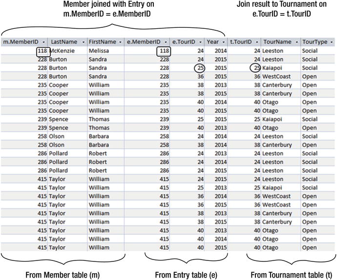
Figure 3-7. Joining the Member, Entry, and Tournament tables

The join condition for the first join between the Member and Entry tables is that m.MemberID = e.MemberID as shown by the rectangular boxes in Figure 3-7. For the second join between the result of the first join and the Tournament table, the condition is that e.TourID = t.TourID as shown by the circles. It will not make any difference if we choose to do the join between Entry and Tournament first and then join the result to Member.

The SQL to carry out the two joins is:

SELECT *
FROM (Member m INNER JOIN Entry e ON m.MemberID = e.MemberID)
      INNER JOIN Tournament t ON e.TourID = t.TourID;

The virtual table resulting from the two joins in this query has all the information we require to answer our question. We just need to select the rows satisfying the conditions about the year and tournament name by adding a WHERE clause, and then project the name attributes by specifying them in the SELECT clause. The complete SQL query to return the names of everyone who entered the Leeston tournament in 2014 is:

SELECT LastName, FirstName
FROM (Member m INNER JOIN Entry e ON m.MemberID = e.MemberID)
      INNER JOIN Tournament t ON e.TourID = t.TourID
WHERE TourName = 'Leeston'
AND Year = 2014;

Order of Operations

In the description in the previous section, we joined all the tables first and then selected the appropriate rows and columns. The result of the join is an intermediate table (as in Figure 3-7) that is potentially extremely large if there are lots of members and tournaments. We could have done the operations in a different order. We could have first selected just the Leeston tournament from the Tournament table and the 2014 tournaments from the Entry tables, as shown in Figure 3-8. Joining these two smaller tables with each other and then joining that result with Member would result in a much smaller intermediate table.

Figure 3-8. Selecting rows from the Entry and Tournament tables before joining them

So, should we worry about the order of the operations? The answer is “yes” — the order of operations makes a huge difference — but if you are using SQL, then it is not your problem to worry about. The SQL statement is always going to be the same, but with the tables possibly in a different order. The SQL statement is sent to the engine of whatever database program you are using, and the query will be optimized. This means the database program figures out the best order to do things. Some products do this extremely well, others not so well. Many products have analyzer tools that will let you see in what order things are being done. For many queries, writing your SQL differently doesn’t make much difference, but you can make things more efficient by providing indexes for your tables. We will look at these issues more closely in Chapter 9.

An Outcome Approach

The reason that the way we write our SQL statements often doesn’t affect the efficiency of a query is that SQL is fundamentally based on relational calculus, which describes the criteria the retrieved rows must meet. The original SQL standards did not even have keywords like INNER JOIN. SQL statements without these keywords describe what the retrieved rows should be like, so they do not have anything to say about how. Let’s look at an outcome approach to finding the names of members who entered Leeston tournaments in 2014.

We want to retrieve just some names from the Member table. Forget joins, and think about how you would know whether a particular name should be retrieved if you were shown the three tables and knew nothing about databases or foreign keys or joins or anything. Imagine a finger m tracing down the table, as in Figure 3-9.

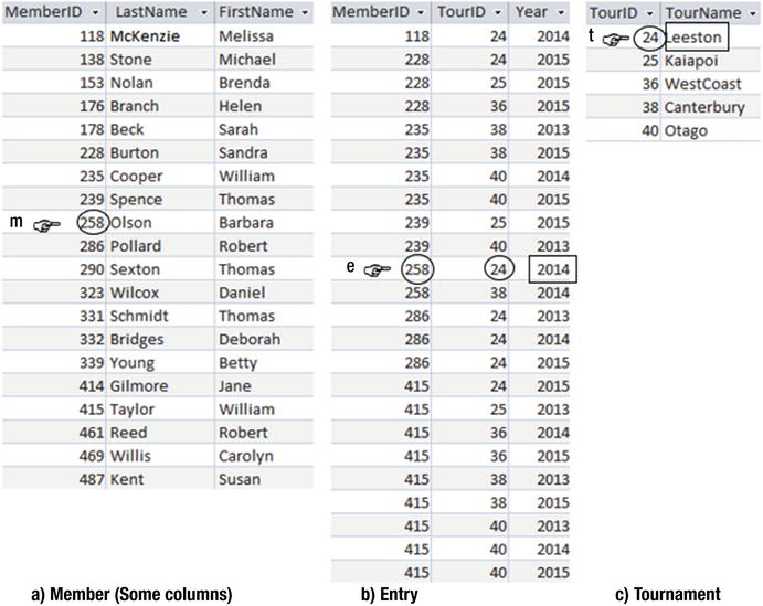
Figure 3-9. Using row variables to describe the rows that satisfy the query conditions

Do we want to write out Barbara Olson, the name to which m is currently pointing? How would we know? Well, first we have to find a row with her ID (235) in the Entry table for the year 2014 such as the one where finger e is pointing. Then we have to find a row with that tournament ID (24) in the Tournament table and check it is a Leeston tournament. Looking at Figure 3-9, we see that the rows where the three fingers are pointing give us enough information to know that Barbara Olson did indeed enter a Leeston tournament in 2014. This set of conditions describes what a row in the result table should be like.

Now let’s write that last paragraph a bit more succinctly. Read the following sentence with reference to the rows denoted in Figure 3-9:

I’ll write out the names from row m , where m comes from the Member table, if there is a row e in the Entry table where m.MemberID is the same as e.MemberID and e.Year is 2014 and there also exists a row t in the Tournament table where e.TourID is the same as t.TourId and t.TourName has the value “Leeston.”

The SQL reflects the preceding paragraph. Look carefully at the following statement with reference to Figure 3-9:

SELECT m.LastName, m.FirstName
FROM Member m, Entry e, Tournament t
WHERE m.MemberID = e.MemberID
      AND e.TourID = t.TourID
      AND t.TourName = 'Leeston' AND e.Year = 2014;

You can see how the SQL statement describes what a retrieved row should be like. If you look carefully at the statement, you can also spot the operations. The second line (the FROM clause) is a big Cartesian product, the next two lines are the join conditions (which would result in a table like the one in Figure 3-7), the final line selects the rows with the appropriate year and tournament name, and the SELECT clause line tells us to project just the names.

The SQL preceding statement is equivalent to the one using the INNER JOIN keywords. They will both return the same set of rows: one reflects the underlying process of how, and the other reflects the underlying outcome of what.

Expressing Joins Through Diagrammatic Interfaces

This book is about queries in SQL, but most database products also provide a diagrammatic interface to express queries. Just for completeness, I’ll show you what a typical diagrammatic interface looks like for retrieving the names of members who entered the Leeston tournament in 2014.

Figure 3-10 shows the Microsoft Access interface, but most products have something very similar. The tables are represented by the rectangles in the top section with the lines showing the joins between them. The columns to be retrieved have a checkmark (√) in the row marked Show, and the conditions for selecting a particular row are shown for the relevant fields in the row marked Criteria.

Figure 3-10. Microsoft Access digrammatic interface for the query to find names of members entering the Leeston tournament in 2014

Outer Joins

One type of join that you will use a great deal and that is important to understand is the outer join. The best way to understand an outer join is to see where they are useful. Have a look at the (modified) Member and Type tables in Figure 3-11.

Figure 3-11. Member and Type tables

You might want to produce different lists from the Member table, such as numbers and names, names and membership types, and so on. In these lists you expect to see all the members (for the table in Figure 3-11, that would be nine rows). Then you might think that as well as seeing the numbers and names in your member list, you will also include the membership fee. You join the two tables (with the condition MemberType = Type) and find that you “lose” one of your members — Sarah Beck (see Figure 3-12).

Figure 3-12. Inner join between Member and Type, and we “lose” Sarah Beck

The reason is that Sarah has no value for MemberType in the Member table. Let’s look at the Cartesian product, which is the first step for doing a join. Figure 3-13 shows those rows of the Cartesian product that include Sarah.

Figure 3-13. Part of the Cartesian product between the Member and Type tables

Having done the Cartesian product, we now need to do the final part of our join operation, which is to apply the condition (MemberType = Type). As you can see in Figure 3-13, there is no row for Sarah Beck that satisfies this condition because she has a null or empty value in MemberType.

Consider the following two natural-language questions: “Get me the fees for members” and “Get me all member information including fees.” The first one has an implication of “Just get me the members who have fees,” while the second has more of a feel of “Get me all the members and include the fees for those who have them.” One of the biggest difficulties in writing queries is trying to decide exactly what it is you want. It is even more difficult if you are trying to understand what someone else is asking for!

Let’s say that what we actually want is a list of all our members, and where we can find the fee information, we’d like to include that. In this case, we want to see Sarah Beck included in the result, but with no fee displayed. That is what an outer join does. Outer joins can come in three types: left, right , and full outer joins. A left outer join retrieves all the rows from the left table including those with a null value in the join field, as shown in Figure 3-14. We see that as well as all the rows from the inner join (Figure 3-12), we also have a row from the Member table for Sarah, who had a null for the join field MemberType. The fields in that row that would have come from the right-hand table (Type and Fee) have null values.

Figure 3-14. Result of left outer join between Member and Type tables

The SQL for the outer join depicted in Figure 3-14 is similar to an inner join, but the key phrase INNER JOIN is replaced with LEFT OUTER JOIN (or in some applications simply LEFT JOIN):

SELECT *
FROM Member m LEFT OUTER JOIN Type t ON m.MemberType = t.Type;

You might quite reasonably say that we wouldn’t have needed an outer join if all the members had a value for the MemberType field (as they probably should). That may be true for this case — but remember my cautions in Chapter 2 about assuming that fields that should have data will have data. In other situations, the data in the join field may be quite legitimately empty. We will see in later chapters queries like “List all members and the names of their coaches — if they have one.” “Losing” rows because you have used an inner join when you should have used an outer join is a very common problem and is sometimes quite hard to spot.

What about right and full outer joins? Left and right outer joins are the same and just depend on which order you put the tables in the join statement. The following SQL statement will return the same information as displayed in Figure 3-14, although the columns may be presented in a different order:

SELECT *
FROM Type t RIGHT OUTER JOIN Member m ON m.MemberType = t.Type;

We have simply swapped the order of the tables in the join statement. Any rows with a null in the join field of the right table (Member) will be included.

A full outer join will retain rows with a null in the join field in either table. The SQL for the full outer join is shown here and will result in the table seen in Figure 3-15:

Figure 3-15. Result of a full outer join between Member and Type tables

SELECT *
FROM Member m FULL OUTER JOIN Type t ON m.MemberType = t.Type;

We have a row for Sarah Beck padded with mull values for the missing columns from the Type table. We also have the first row, which shows us the information about the Associate membership type even though there are no rows in the Member table with Associate as a member type. In this row, each missing value from the Member table is replaced with a null.

Not all implementations of SQL have a full outer join implemented explicitly. Access 2013 doesn’t. However, there are always alternative ways in SQL to retrieve the information you require. In Chapter 7 I’ll show you how to get the equivalent of a full outer join by using a union operator between a left and right outer join (which is what I had to do to get the screen shot in Figure 3-15!).