
SQL (Structured Query Language) enables us to create tables, apply constraints, and manipulate data in a database. In this book we will concentrate on queries that allow us to extract information from a database by describing the subset of data we need. That data might be a single number , such as a product price, a list of the names of members with overdue subscriptions, or a calculation, such as the total dollar amount of products sold in the past 12 months. In this book we will be looking at different ways to approach a query so that it can be expressed correctly in SQL.
Before getting into the nuts and bolts of how to specify queries, we will review some of the ideas and terminology associated with relational databases. We will also look at data models, which are a succinct way of depicting how a particular database is put together, that is, what data is being kept where and how everything is interrelated.
It is imperative that the underlying database has been designed to accurately represent the situation it is dealing with. This means not only that suitable tables have been created, but also that appropriate constraints have been applied so that the data is consistent and stays consistent as the database evolves. Even with all the fanciest SQL in the world, you are unlikely to get accurate responses to queries if the underlying database design is faulty. If you are setting up a new database, you should refer to a design book1 before embarking on the project.
Introducing Database Tables
In simple terms, a relational database is a set of tables.2 Each table in a well-designed database keeps information about aspects of one thing, such as customers, sales, teams, or tournaments. Throughout the book we will base the majority of the examples on a database for a golf club. The tables will be introduced as we progress, and an overview is provided in Appendix 1.
Attributes
When a table is created we need to specify what information it will hold. For example, a Member table might contain information about names, addresses, and contact details. We need to decide what the individual pieces of data will be. For example, we might choose to separate the name information into a title, a first name, a family name, initials, and a preferred name. This type of separation allows us more flexibility in how the data is used. For example, we can address correspondence to Mr. J. A. Stevens and start the message with Dear Jim. Each of these separate pieces of information is an attribute of the table.
To define an attribute we need to provide a name (e.g., FamilyName, Handicap, or DateOfBirth) and a domain or type. A domainis a set of allowed values and might be something very general or something quite specific. For example, the domain for columns storing dates might be any valid date (so that February 29 is allowed only in leap years), whereas for columns keeping quantities the domain might be integer values greater than 0. We might initially think that the domain for a FamilyName attribute could be any string of characters, but on reflection we will need to consider whether some punctuation is allowed (probably yes), if numbers are permitted (hard to say), and if there should be a minimum or maximum length. All database systems have built-in domains or types such as text, integer, or date that can be chosen for each of the fields in a table. More sophisticated products allow the user to define their own types, which can be used across tables. For example, we might define a type called CarRegistration that has a predetermined template of letters and digits. Even if it is not possible to define your own types, all good database systems allow the designer to specify constraints on a particular attribute in a table. For example, in a particular table we might specify that a birthdate is a date in the past or that a handicap is between 0 and 40. Some attributes might be allowed to be empty, while others may be required to have a value.
When we view the table, the names of the attributes are the column headers, and the domain or type provides the set of allowed values. Once we have defined the table we add data by providing a row for each instance. For example, if we have a Member table , as in Figure 1-1, each row represents one member.
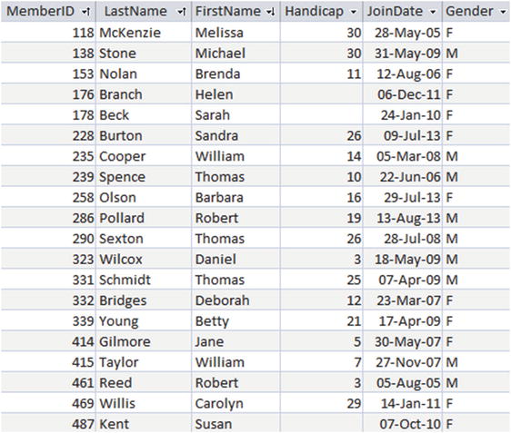
Figure 1-1. The Member table
The Primary Key
One of the most important features of a relational database table is that each of its rows should be unique. No two rows in a table should have identical values for every attribute. If we consider our member data, it is clear why this uniqueness constraint is so important. If, in the table in Figure 1-1, we had two identical rows (say, for Brenda Nolan), we would have no way to differentiate them. We might associate a team with one row and a subscription payment with the other, thereby generating all sorts of confusion.
The way that a relational database maintains the uniqueness of rows in a table is by specifying a primary key . A primary key is an attribute, or set of attributes, that is guaranteed to be different in every row of a given table. For data such as the member data in this example, we cannot guarantee that all our members will have different names or addresses (a father and son may share a name and address and both belong to the club). It is important that there are sufficient attributes to be able to distinguish the rows in a table. Adding a birthdate would resolve the problem mentioned above. Dealing with large numbers of attributes as a primary key can become cumbersome, so to help distinguish different members, we have included an ID number as one of the attributes in the table in Figure 1-1. We can now uniquely identify a member by specifying their ID. This has the added advantage that we can also keep track of members if they change their names. Adding an identifying number (sometimes referred to as a surrogate key) is very common in database tables. If MemberID is defined as the primary key for the Member table, then the database system will ensure that in every row the value of MemberID is different. The system will also ensure that the primary key field always has a value. That is, we can never add a row that has an empty MemberID field. These two requirements for a primary key field (uniqueness and not being empty) ensure that given a value for MemberID, we can always find a single row that represents that member. We will see that this is also important when we start looking at relationships between tables later in this chapter.
The code that follows shows the SQL code for creating the Member table shown in Figure 1-1. Each attribute has a name and type specified. In SQL, the keyword INT means an integer or non-fractional number, and CHAR(n) means a string of characters n long. The code also specifies that MemberID will be the primary key. Every table in a well-designed database should have a primary key clause.
CREATE TABLE Member (MemberID INT PRIMARY KEY,LastName CHAR(20),FirstName CHAR(20),Handicap INT,JoinDate DATETIME,Gender CHAR(1));
Inserting and Updating Rows in a Table
The emphasis of this book is on getting accurate information out of a database, but the data first has to get in somehow. Most database application developers will provide user-friendly interfaces for inserting data into the various tables. Often a form is presented to the user for entering data that may end up in several tables. Figure 1-2 shows a simple Microsoft© Access form that allows a user to enter and amend data in the Member table.
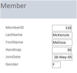
Figure 1-2. A form allowing entry and updating of data in the Member table
It is possible to construct web forms or use mechanical readers, such as bar-code readers, that can collect data and insert it into a database. Data can also be added with bulk updates from files or be imported from other applications. Behind all the different mechanisms for updating data, SQL update queries are generated. We will see three types of queries for inserting or changing data just to get an idea of what they look like.
The code that follows shows the SQL to enter one complete row in our Member table. The data items are in the same order as specified when the table was created. Note that the date and string values need to be enclosed in single quotes.
INSERT INTO MemberVALUES (118, 'McKenzie', 'Melissa', '963270', 30, '05/10/1999', 'F')
If many of the data items are empty, we can specify which attributes will have values. If we had only the ID and last name of a member, we could insert just those two values as shown here:
INSERT INTO Member (MemberID, LastName)VALUES (258, 'Olson')
When adding a new row as just seen, we always have to provide a value for the primary key.
We can also alter records that are already in the database with an update query. The following query will find the row for the member with ID 118 and then will update the phone number:
UPDATE MemberSET Phone = '875077'WHERE MemberID = 118
This query specifies which rows are to be changed (the WHERE clause) and also specifies the field to be updated (the SET clause).
Designing Appropriate Tables
Even a quite modest database system will have hundreds of attributes: names, dates, addresses, quantities, prices, descriptions, ID numbers, and so on. These all have to find their way into tables, and getting them in the right tables is critical to the overall accuracy and usefulness of the database. Many problems can arise from having attributes in the “wrong” tables. As a simple illustration of what can go wrong, I’ll briefly show the problems associated with having redundant information.
Say we want to add teams and practice nights to the information we are keeping about members of our golf club. We could add these two fields to the Member table, as in Figure 1-3.
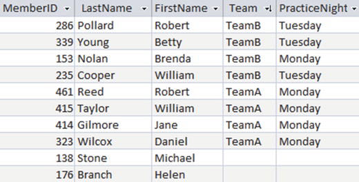
Figure 1-3. Possible Member table
Immediately, we can see there has been a problem with the data entry because Brenda Nolan has a practice night that is different from the rest of her team members. The piece of information about the practice night for each team is being stored several times, so inevitably inconsistencies will arise. If we formulated a query to find the practice night for TeamB, what would we expect for an answer? Should it be Monday, Tuesday, or both?
The problem here is that (in database parlance) the table is not properly normalized. Normalization is a formal way of checking whether attributes are in the correct table. It is outside the scope of this book to delve into normalization, but I’ll just briefly show you how to avoid the problem in this particular case.
The problem is that we are trying to keep information about two different things in our Member table: information about each member (IDs, names, and so on) and information about teams (the practice nights). The PracticeNight attribute is in the wrong table. Figure 1-4 shows a better solution with two tables: one for information about members and one for information about teams.
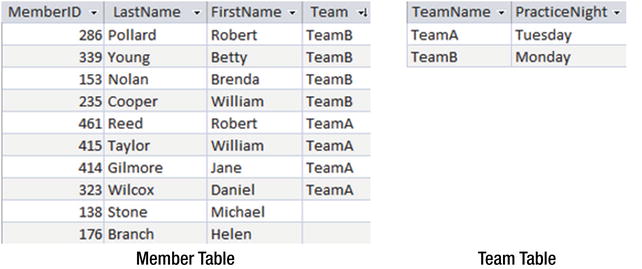
Figure 1-4. Member and Team tables
This separation of information into two tables prevents the inconsistent data we had previously. The practice night for each team is stored only once. If we need to find out what night Brenda Nolan should be at practice, we now need to consult two tables: the Member table to find her team and then the Team table to find the practice night for that team. The bulk of this book is about how to do just that sort of data retrieval.
Introducing Data Models
Even the simplest databases are likely to have several tables. A data model is a conceptual model of the underlying data and how it is interrelated. We will use the class diagram notation from the Unified Modeling Language (UML )3 to represent our data models. There are many other ways to represent data structure (for example, Entity Relationship Diagrams) that, for the purposes of this book, would also be suitable. We choose to use UML as it has a large suite of diagramming tools for developing software applications that encompasses not only the structure of data but also its behavior. In this section, we will look at how to interpret a class diagram and how to translate it into tables and constraints in a relational database.
A class is like a template for something we want to keep data about (events, people, places, etc.) For example, we might want to keep names and other details about the members of our golf club. Figure 1-5 shows the UML notation for a Member class . The name of the class is in the top panel, and the next panel shows the attributes. Class diagrams can also have another panel to show methods associated with the behavior of the class.
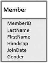
Figure 1-5. UML representation of a Member class
In a relational database, each class is represented as a table, the attributes are the columns, and each instance (in this case an individual club member) will be a row in the table.
The data model can also depict the way the different classes depend on each other. Figure 1-6 shows two classes, Member and Team, and how they are related.
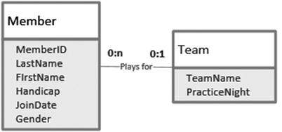
Figure 1-6. A relationship between two classes
The pair of numbers at each end of the plays for line in Figure 1-6 indicates how many members play for one particular team, and vice versa. The first number of each pair is the minimum number. This is often 0 or 1 and is therefore sometimes known as the optionality(that is, it indicates whether a member must have an associated team, or vice versa). The second number (known as the cardinality) is the greatest number of related objects. It is usually 1 or many (denoted by n or *), although other numbers are possible.
Relationships can be interpreted in both directions. The label on the relationship in Figure 1-6 implies that we are reading from left to right and we will need to think of the appropriate verb for interpreting the diagram in the other direction. “Team has members” will do. Reading Figure 1-6 from left to right, we see that one particular member doesn’t have to play for a team and can play for at most one team (the numbers 0 and 1 at the end of the line nearest the Team class). Reading from right to left, we can say that one particular team doesn’t need to have any members but can have many (the numbers 0 and n nearest the Member class). A relationship like the one in Figure 1-6 is called a 1–Many relationship (a member can belong to just one team, and a team can have many members).
You might think there should be exactly four members for a team (say, for an interclub team). Although this might be true when the team plays a round of golf, our database might record different numbers of members associated with the team as we add and remove players throughout the year. A data model usually uses 0, 1, and many to model the relationships between tables. Other constraints (such as the maximum number on a team) are more usually expressed with business rules or with UML use cases.4
We can represent a 1-Many relationship in our database by looking at the primary key at the 1 end of the relationship and adding a column of the same type to the table at the Many end. For the model in Figure 1-6 we would add a Team column to the Member table as shown in Figure 1-7.
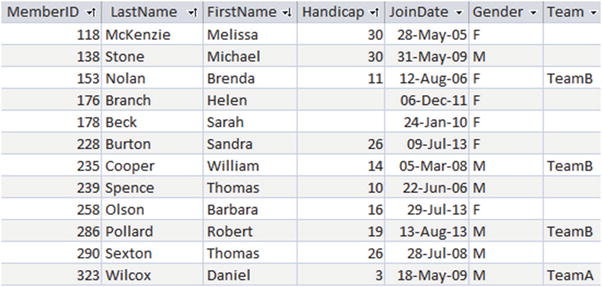
Figure 1-7. Member table with a foreign key column Team
The Team column is called a foreign key. Any non-empty value in this column in the Member table must be a value that already exists in the primary key column of the Team table. The concept of a foreign key provides us with a constraint on the Member table so that we cannot assign members to non-existent teams. This constraint is called referential integrity.
The SQL to create a table with a foreign key is shown here:
CREATE TABLE Member(MemberID INT PRIMARY KEY,LastName CHAR(20),FirstName CHAR(20),Phone CHAR(20),Handicap INT,JoinDate DATETIME,Gender CHAR(1),Team CHAR(20) FOREIGN KEY REFERENCES Team);
Because we need to compare the value in the foreign key column of the Member table with the primary key column of the Team table, these two columns must have the same domain or datatype.
Most database products have a graphical interface for setting up and displaying foreign key constraints. Figure 1-8 shows the interfaces for Microsoft© SQL Server and Microsoft© Access. These diagrams, which are essentially implementations of the data model, are invaluable for understanding the structure of the database so we know how to extract the information we require.
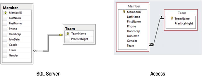
Figure 1-8. Diagrams for implementing 1–Many relationships using foreign keys
The tables in Figures 1-4 and 1-7 have essentially the same design. For Figure 1-4 we arrived at the design by removing the PracticeNight column from the Member table and creating a new Team table (a normalization process). For Figure 1-7 we first considered a data model and added the Team column to the Member table as a way of representing the relationship between Member and Team. The outcome is the same whichever way you approach the issue.
At the risk of repeating myself, I do want to caution about the necessity of ensuring that the database is properly designed. The simple model in Figure 1-6 is almost certainly quite unsuitable even for the tiny amount of data it contains. A real club will probably want to keep track of how the membership of teams evolves over the years. This will involve including information about seasons or years along with the team membership information. Some members might play for more than one team during a year if they are called in as a substitute . That information may or may not be necessary to retain. Designing a useful database is a tricky job and outside the scope of this book.5
Retrieving Information from a Database
Now that we have a well-designed database consisting of interrelated normalized tables, we can start to look at how to extract information by way of queries. When I refer to extracting or retrieving information I don’t mean that we are removing any data. Think of a query as providing a window onto a small part of the database. Many database systems will have a diagrammatic interface that can be useful for simple queries. Figure 1-9 shows the Microsoft© Access interface for retrieving the names of senior members from the Member table. The checkmarks denote which columns we want to retrieve, and the Criteria row enables us to specify conditions on the rows that are returned.
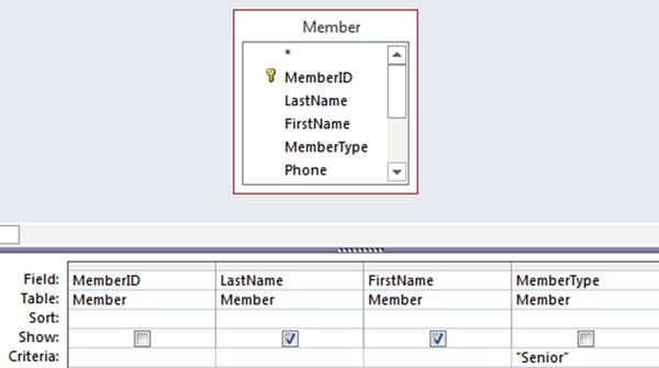
Figure 1-9. Access interface for a simple query on the Member table
The application will take the information from the graphical interface and construct an SQL query. Most applications will show you the SQL that is generated, and you can amend it or write it from scratch yourself. The SQL equivalent to the query depicted in Figure 1-9 is:
SELECT FirstName, LastNameFROM MemberWHERE MemberType = 'Senior';
This SQL query contains three clauses: SELECT specifies which columns to return, FROM specifies the table(s) where the information is kept, and WHERE specifies the conditions the returned rows must satisfy. We’ll look at the structure of SQL statements in more detail later, but for now the intention of the query is pretty clear.
As we need to include more and more tables connected in a variety of ways, the diagrammatic interfaces rapidly become unwieldy, and often we need to write the SQL commands directly. Often, it is easier to think about a query in a more abstract way. With a clear abstract understanding of what is required, it then becomes more straightforward to turn the idea into an appropriate SQL statement. There are two different ways to approach queries on a relational database.
Process Approach
One way to approach a query is to think in terms of the operations we need to carry out on the tables. Let’s think about how we might to get a list of names for members who practice on a Monday. We might imagine first retrieving just the rows from the Team table that have Monday in the PracticeNight column. We might then join those rows with the Member table (more about joins later) and then extract the names from the result. We will call this the process approach, as it is a series of steps carried out in a particular order. Figure 1-10 depicts the steps just described.
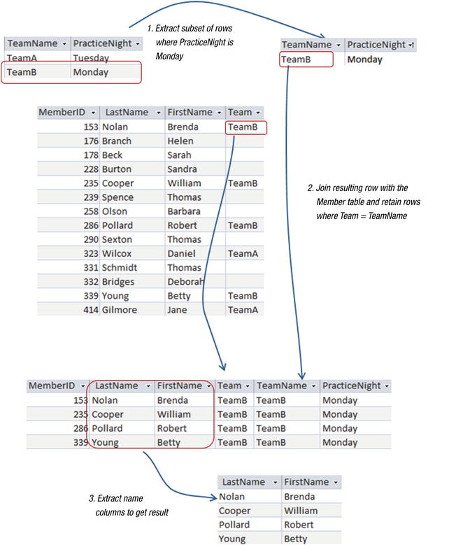
Figure 1-10. The process approach: thinking of a query as a sequence of operations
Outcome Approach
An alternative way to think about the query in the previous section is to examine all the rows in the Member table and just return those that satisfy the criteria that the member is on a team that has Monday as a practice night. Figure 1-11 depicts this train of thought. The row m that we are considering in the Member table satisfies the condition about the team’s practice night, so we should retrieve the names from that row.
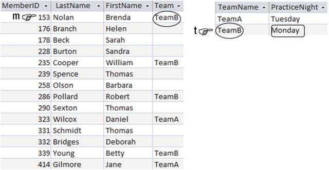
Figure 1-11. Considering if the row m satisfies the criteria for the query.
We will call this type of thinking about a query the outcome approach because we describe what we want rather than how to get it.
Why We Consider Two Approaches
Relational database theory has its origins in set theory. If we think of our tables as sets of rows, then a query is a question that requires us to manipulate those sets to retrieve a subset containing the information we require. The relational theory has two formal ways of specifying the criteria for extracting subsets of rows: relational algebra and relational calculus .
We do not need these abstract ideas for simple queries. However, if all queries were simple, you would not be reading this book. In the first instance, queries are expressed in everyday language that is often ambiguous. Try this simple expression: “Find me all students who are younger than 20 or live at home and get an allowance.” This can mean different things depending on where you insert commas. For example a comma after “20” leads to the interpretation that everyone under 20 is included, while a comma after “home” suggests that they must also get an allowance. Even after we have sorted out what the natural-language expression means, we then have to think about the query in terms of the actual tables in the database. This means having to be quite specific in how we express the query. Both relational algebra and relational calculus give us a powerful way of being accurate and specific.
Why not skip all this abstract stuff and go right ahead and learn SQL? Well, the SQL language consists of elements of both calculus and algebra. Older versions of SQL were purely based on relational calculus in that you described what you wanted to retrieve rather than how. Modern implementations of SQL allow you to explicitly specify algebraic operations such as joins, unions, and intersections on the tables as well.
There are often several equivalent ways of expressing an SQL statement. Some ways are very much based on calculus, some are based on algebra, and some are a bit of both. During my time as a university lecturer I often asked the class whether they found the calculus or algebra expressions more intuitive for a particular query. The class was usually equally divided. Personally, I find that some queries just feel obvious in terms of relational algebra, whereas others feel much more simple when expressed in relational calculus. Once I have the idea pinned down with one or other, the translation into SQL (or some other query language) is usually straightforward.
We can make use of the ideas of relational algebra and relational calculus without delving into the mathematics. In the body of the book I refer to the process approach(algebra) and the outcome approach(calculus). The more tools you have at your disposal, the more likely it is that you will be able to express complex queries accurately. In Appendix 2 there is an introduction to the formal notation for relational algebra and relational calculus for those of you who would like to add that to your armory.
Summary
This chapter has presented an overview of relational databases. We have seen that a relational database consists of a set of tables that represent the different aspects of our data (for example, a table for members and a table for teams). The attributes needed to describe the members or teams become the columns of the tables, and each column has a set of allowed values (a domain). Each table should have a primary key, which is an attribute or set of attributes guaranteed to have a different value for every row.
It is possible to set up constraints between tables with foreign keys. A foreign key is a value for a column(s) in one table that has to already exist as a value in the primary key column(s) of another table. For example, the value of Team in the Member table must be one of the values in the primary key field of the Team table.
It is often helpful to think about queries in an abstract way, and there are two ways to do this. The process approach requires us to think about the operations that can be applied to tables in a database. It is a way of describing how we need to manipulate the tables to extract the information we require. The outcome approach requires us to think about what criteria our required information must satisfy. Different people will find that one or the other of these approaches feels more natural for different queries. SQL is a language for specifying queries on a database. There are usually many equivalent ways to specify a query in SQL. Some reflect the process approach and some reflect the outcome approach — and some are a bit of both.
Footnotes
1 For example, you can refer to my other Apress book, Beginning Database Design: From Novice to Professional (New York: Apress, 2012).
2 More correctly, it’s a set of relations. In the body of the book common words such as table and row are used. In Appendix 2 we introduce the more formal vocabulary and notation.
3 If you want more information about UML, then refer to Grady Booch, James Rumbaugh, and Ivar Jacobsen, The Unified Modeling Language User Guide (Boston, MA: Addison Wesley, 2005). The current standards can be found at http://www.uml.org/ .
4 Alistair Cockburn, Writing Effective Use Cases (Boston, MA: Addison Wesley, 2001).
5 For more information about database design, refer to my other Apress book, Beginning Database Design: From Novice to Professional (New York: Apress, 2012).