You may not need to read this chapter! Database management systems (DBMS) are very efficient, and if you have a modest amount of data, most of your queries will probably be carried out in the blink of an eye. Complicating your life in an attempt to make your queries a little faster does not make a great deal of sense. However, if you have (or might have) vast amounts of data and speed is absolutely critical, you will need more skill and experience than you are likely to get from reading one chapter in a beginners’ book. Having said that, you are likely to have people tell you that it matters how you express your queries or that you should be indexing your tables, so it is handy to have some idea about what is going on behind the scenes and understand some of the terminology.
Throughout this book, I have emphasized that there are often alternative ways to phrase a query in SQL. The implementation of SQL you are using may not support some constructions, so your choices may be limited. Even then, you usually have alternatives for most queries. Does it matter which one you use? One consideration is the transportability of your queries. If you are unsure where your query may be used, you might choose to avoid keywords and operations that are not widely supported (yet). However, typically you will be writing queries for a database with a specific implementation of SQL. In that case, your main questions are “How will the different constructions of a query affect the performance?” and “Is there anything I can do to improve performance?”
What Happens to a Query
Up to this point we have been concentrating on taking a question we need answered and constructing a query that will return appropriate and accurate information from the database. Conceptually the query writer thinks of the database as being a collection of tables. An SQL statement is an expression describing which data should be retrieved from those tables and what constraints that data must obey (the outcome approach).1
We have also seen that a query can be specified by describing set operations, such as joins and intersections, which would result in the appropriate data being returned (the process approach). Using set operations makes forming a query very elegant, but the operations are purely conceptual. While we might specify the query in terms of, say, a join followed by an intersection, this will be interpreted by the DBMS as a description of the data to be returned not as a method for retrieving the data.
The ideas of tables and data models is a useful way for us to understand how the pieces of data are logically related. We leave it to the DBMS to take care of how the data is physically stored and retrieved. Figure 10-1 is a simplified schematic of the different levels of abstraction that can help us understand a database.
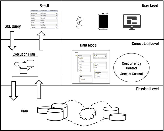
Figure 10-1. Levels of a database management system
At the top of the diagram in Figure 10-1 we have the user level. This is where we have the different applications and devices that form the interface between the humans and the data. It is here that a user (or application) will construct an SQL statement (top left of the diagram).
The middle layer is a conceptual view of the database. We can think of the data as being in tables with various key and validation constraints. It is also where we can form models of how the database should deal with concurrent users and the rules for allowing access to different data. The SQL statements we construct are in terms of all these concepts.
The actual data is stored in the physical level, shown at the bottom of Figure 10-1. What we think of as a table may be segments of data stored on possibly different servers maybe in different countries. At this level there will be indexes that allow rapid access to different records; we will talk about those in later sections of this chapter.
How the relevant pieces of information are located and assembled to produce the result of the query is a job for the query optimizer. The SQL statement constructed by the user is passed to the optimizer, which has access to information about the number of rows in a (conceptual) table, the amount of data in each row, the attributes on which indexes have been created, and so on. It uses all this information to create an execution plan. The execution plan is an efficient sequence of steps to find, compare, and assemble the data into the result specified by the query. The data is retrieved from physical storage and assembled in accordance with the execution plan, and the result is returned to the user — usually in the form of a table.
Most commercial database software provides tools for displaying proposed execution plans and the estimated times for each step to be carried out. This provides insight into how a query is being executed and where the time is being spent. A good database administrator will be able to use this type of information to tune the database; for example, by adding new indexes.
In the following sections, we will take a brief look at how records are stored, how indexes can improve efficiency, and some of the things that go on behind the scenes when a query is carried out.
Finding a Record
Most of the queries on a database will, at some point, involve finding records that match a particular condition. For example we may want to find records in a single table (e.g., WHERE LastName = 'Smith'), find records from two tables that match a join condition (e.g., WHERE m.MemberID = e.MemberID), or look for the existence or otherwise of values (e.g., WHERE NOT EXISTS... ).
Searching for and finding data all seems pretty easy these days when everything is stored electronically. If we want to find a topic in an online book we just open a search box and type in some keywords. With a physical book it is a very different story. We either have to scan through every page or hope there is a useful index or table of contents. Those who remember physical telephone books will recall that it was easy to find Jim Smith but impossible to find who lives at 16 Murray Place.
Behind the scenes in a database the issues are the same as for physical books. The data can only be stored in one order, but we might want to search it in a variety of ways. It is useful to know what is actually going on so that we have an understanding of what affects the performance of locating a specific record.
One way to find records matching a condition is to simply look sequentially through every row in the table. This is the slowest and costliest way to find what you are looking for. Having said that, it may not be a problem. It would not take long to scan the golf club Type table to find the membership fee for seniors. On the other hand, it would be a bigger job to scan every row in (a realistic) Entry table to find members who had entered tournament 38 over the last forty years.
Storing Records in Order
If we consider relational theory, then the rows in a table2 have no order. This allows us to consider a table as a set and apply all the set operations. This is useful from a conceptual point of view, but in practice how the records are stored is going to make a difference in how quickly we can find what we are looking for.
If the records of a table are stored in a random order (perhaps the order they were created) then this is referred to as a heap table. The only way to find a record in a heap table is to scan the entire table. Generally the records will be stored ordered by some attribute(s) — often the primary key. There are all sorts of algorithms for finding a particular record quickly in an ordered table, but most will be built on the idea of a binary search.
When we try to find a name in a telephone book or a word in a dictionary we employ a type of binary search. In the simplest scenario we inspect a page in the middle of the book and decide if the target word is before or after the words on that page. We then start again and inspect a page halfway through the portion that is of interest. Very quickly we zero in on the page required. If the records in a table are ordered by a particular field, then searches on that field will be more efficient than searches on fields with no index.
When we talk about records in a table being stored in order, we don’t mean they are physically one after the other on a disc. If this were the case then if we wanted to insert a new record near the beginning we would have to move all the others along. The records can be thought of as being in a tree-like structure. One common type of tree is a B-Tree. Figure 10-2 shows a very simple representation of a B-Tree structure for storing letters of the alphabet.
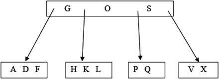
Figure 10-2. Representation of data in a B-Tree
If you are searching for a letter in the tree in Figure 10-2 you would start at the top node, or box. In the top node you either find what you are looking for or you follow the appropriate path. For example, if you are looking for H you would follow the path between G and O. The structure allows records to be added and deleted with the minimum of disruption. We can easily add R to the box containing P and Q without altering any of the other letters. Maintaining a B-Tree is not trivial. As data is added and removed the tree will need to be rearranged to keep it balanced and to add and remove nodes and levels. Fortunately, all this goes on under the hood.
Having said all that, when we are thinking about records being in order it is usually easiest to imagine them all in a single line. That is what I will do for the rest of this chapter.
Clustered Index
If the records are physically stored in some order then this is referred to as a clustered index. If we thought it a good idea to store our member records in order of names, we could specifically create a clustered index so that the records are stored in order of the value of LastName. We can create an index with an SQL statement. We need to provide a name for the index (e.g., Clustered_Name) and specify the field(s) on which to order the index, as in the query here:
CREATE CLUSTERED INDEX Clustered_Name ON Member (LastName);By default, the order for a clustered index is usually the value of the primary key. While it is possible to specify a different order for the clustered index, you need to have a good reason to do so.
With a clustered index in place, there are now two ways to locate a record. Consider running the following query on the Member table with the clustered index on LastName:
SELECT *FROM MEMBER WHERE LastName = 'Smith';
Because the table is in order of LastName we can quickly navigate to the correct record by doing a binary search. This is known as a table seek.
Now consider the following query:
SELECT *FROM MEMBERWHERE Phone = '03-567-123';
We have no option now but to check every record in the table. We cannot even stop when we get to a matching record, as there may be several records with the same phone number. This is known as a table scan.
Non-Clustered Indexes
The records in a table can only be stored in one physical order, so there can only ever be one clustered index, which is usually on the primary key. If the clustered index for the Member table is on the primary key field MemberID, we can seek a particular value of MemberID and find the complete row with all the details for that member. If we want to find a row with a particular last name we would have to scan the whole table. Fortunately, we are able to set up additional non-clustered indexes on the table. I’ll refer to these non-clustered indexes as simply indexes from now on. Here is the SQL to create an index on LastName for the Member table:
CREATE INDEX idx_Name ON Member (LastName);What this does is create a list of all the values of LastName in order. Each entry will include a reference to the clustered index so that the full row with the rest of the information can be found. Figure 10-3 illustrates how the first few entries in the LastName index refer to the clustered index.
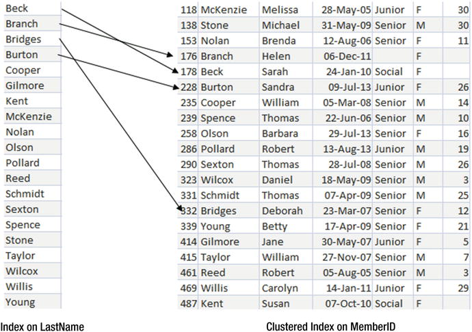
Figure 10-3. Index on LastName has references to clustered index for full information
Because the index is ordered by last name it is possible to do an index seek to find the entry we require and then use the reference to look up the associated row in the clustered index to retrieve the rest of the information.
In practice, whether the query optimizer uses a particular index depends on many factors: the number of rows in the table, the size of each row in the index and the table, whether the records have been accessed recently and have been cached, and so on.
Clustered Index on a Compound Key
Let’s consider the Entry table. Recall that the Entry table has three fields: MemberID, TourIDand Year. Two questions we might ask about the data in this table are:
Which tournament has a particular member entered (say, member 235)?
Who has entered a particular tournament (say, tournament 40)?
It would seem sensible to have two indexes: one on TourID and one on MemberID. However, each of these would refer to the clustered index. What order will that be for the Entry table?
By default, the table will be clustered on the primary key, which for the Entry table is a combination of all three fields. The order of the records will depend on how we specified the primary key. Let’s say the Entry table was created with the following SQL statement:
CREATE Table Entry (MemberID INT,TourID INT,Year INT,PRIMARY KEY (MemberID, TourID, Year);
The order of rows in the clustered index will be as in Figure 10-4. First, they are ordered by the first field specified in the PRIMARY KEY clause (MemberID). Those rows with the same value of MemberID will be ordered by the second field (TourID) and so on.
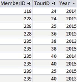
Figure 10-4. Order of data in the default clustered index for the Entry table
The system can easily find the tournaments which member 235 has entered because the entries are in order of MemberID and a table seek can be carried out. We do not necessarily need an additional index on MemberID. On the other hand, finding who has entered tournament 40 would require a scan to investigate every row. In this situation an index on TourID would be an improvement.
The order in which we specify the fields of the primary key can therefore affect how queries are carried out and can influence what other indexes might be useful. Had the order of the primary key fields been specified with PRIMARY KEY (TourID, MemberID, Year) then the clustered index would be in order of TourID. In that case, an index on MemberID should be considered if we regularly need to find rows for a particular member.
I was careful to say for the situation in Figure 10-4 that we might not necessarily need an index on MemberID. The optimizer will take into account many things. One that is important is the size or number of bytes of a typical entry in the index. Each entry in an index made up of two text fields such as LastName and FirstName will be larger than an index on a single text field, which will in turn be larger than an index on a numeric field. Each time an entry in an index is visited it has to be retrieved, so there is an IO (input/output) cost that will depend on the size of the entry.
If the clustered index in Figure 10-3 had significantly more data in each row (e.g., some descriptive text fields) then the cost of retrieving a row would be higher than for retrieving just the three numeric fields. In that case having an index on MemberID would be worth considering. It would not alter how many index entries needed to be investigated, but it would have a smaller IO cost as each entry is smaller. The downside is that once the correct MemberID is located by an index seek the system will need to look up the clustered index to find the rest of the information. Depending on all the information it can access, the optimizer will determine whether it is more efficient to use the index on MemberID and look up the rest of the information, or just to scan all the records in the clustered index.
Updating Indexes
Indexes are clearly wonderfully useful. Why do we not just index everything we are ever likely to search on? This is certainly possible. The downside is that the indexes have to be maintained. Every time we add or delete a record in a table every index on that table will need to be updated also. We therefore have a tradeoff. Lots of indexes will mean fast retrieval but slower updating. Fewer indexes will mean faster updating but possibly slower retrieval.
Managing these tradeoffs is work for an experienced database administrator with excellent knowledge of the domain. There are many tools available that will monitor the database and provide statistics on the use of indexes and other information about the data. If the data is relatively stable with few updates then having several indexes will make retrieval faster. If the data is constantly being updated then indexes may be counterproductive.
In situations where there are a lot of updates it may be practical to do bulk updates of data. With a bulk update you can remove the indexes. The following query shows how to remove the index we created on the Member table earlier in the chapter:
Drop idx_Name on Member;All the additions, deletions, and modifications to the table can then be carried out without the overhead of updating the indexes. At the end of the updates on the table, the indexes can be recreated. This may or may not be more efficient than updating each index for every change.
Covering Indexes
Adding more fields to some indexes can also be effective. Consider the following query:
SELECT FirstNameFROM MemberWHERE LastName = 'Smith'
If the Member table has an index on LastName, then the preceding query would require an index seek to find Smith and then a lookup of the clustered index to find the first name. If the index was on the compound index (LastName, FirstName) then all the information required for the query is contained in the index and no lookup is required. This is known as a covering index. Again, there is the tradeoff of having a larger IO cost for the bigger rows in the index versus the cost of the lookup.
Selectivity of Indexes
Indexes are most useful when the number of rows returned by an index search is small compared to the number of rows in the table.
For example, let’s consider finding information about a member with a particular last name. An index on LastName in the Member table is likely to return only a small percentage of its elements if we search for a specific name. The system can then look up the clustered index for each of those returned elements to retrieve the rest of the information about the members.
By contrast, what happens if we want to find information about women. An index on Gender will return around half its entries if we search for 'F' in the golf club’s Member table. The DBMS would then have to look up the corresponding records in the clustered index. In this situation it is probably more efficient to just scan the clustered index, which contains all the information we require, and not bother with the index at all.
Sometimes the selectivity of an index is not obvious. For example, an index on a field City will not be useful if most of the records in the table have the same value for city and most of the queries are for that city.
Database software often provides tools that can help us. The tools might provide statistics on the current spread of data in fields in a table — for example, what percentage of the table has the same values in a field, such as City. This will help determine if an index might be useful. Often statistics can be collected about how often an index is used. If the optimizer makes little use of an index then it might as well be removed rather than be constantly updated.
Join Techniques
If we consider the Entry table in Figure 10-4, most queries will require a join on the Member table to find the names of the entrants and/or a join on the Tournament table to find the names and other information about the tournaments. Each of these joins compares a foreign key in the Entry table with the primary key of the Member or Tournament table. Refer to Chapter 1 to review what we mean by a foreign key. This joining of a foreign key with a primary key is such a common scenario that it is worth understanding how joins can be carried out. We will use the Member and Entry tables as an example, but the ideas have wide application.
There are a number of different approaches that can be taken when carrying out a join. Which approach will be the most efficient will depend on many things, including the relative sizes of the tables, the indexes that have been created, whether the query also includes projecting specific columns or selecting rows, whether an output order has been specified, and so on. You don’t have to worry about the choice of approach, as that will be decided by the optimizer. However, creating particular indexes can influence the approach taken.
Nested Loops
One approach to joining tables is called nested loops. This means that the system scans one table, and for each row in that table looks through all the rows in the other table to find matches for the join condition. The nested-loop approach is illustrated in Figure 10-5 for the join condition Entry.MemberID = Member.MemberID.
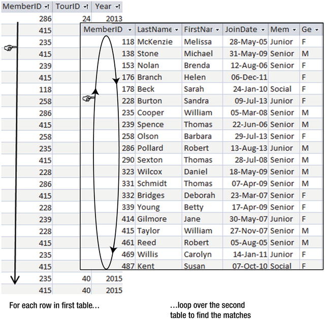
Figure 10-5. Nested-loops approach to finding rows with matching MemberIDs
In Figure 10-5 the outside loop is on the Entry table. For each row in the Entry table, the system will need to find the matching rows in the Member (inner) table. The tables shown in Figure 10-5 are not ordered, which means that every row of the Member table will need to be visited for each row in the Entry table to find the matching records (a table scan).
If there is an index on the matching field in the inner loop (MemberID in the Member table, in this case) then finding the matching field will be more efficient. The index can be used to quickly find the matching records without having to visit every row. In practice, the Member table will probably have a clustered index on its primary key MemberID. If the tables are nested with the Entry table on the inside, then the internal loop will be more effective if there is an index on the MemberID of the Entry table. The optimizer will take this information into account to decide if the nested-loops option is efficient for carrying out the join and which tables should be the inner and outer tables.
Most commercial database systems will provide tools to view the execution plan for a query. Figure 10-6 shows a screenshot from SQL Server showing the execution plan for the join on the Member and Entry tables in the following query:
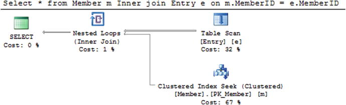
Figure 10-6. Execution plan showing nested loops
SELECT *FROM Member m INNER JOIN Entry e on m.MemberID = e.MemberID;
In Figure 10-6 we see on the top right a table scan of the Entry table. This is the outside loop of the nested loop (as depicted in Figure 10-5). The icon on the bottom right shows that for each row in the Entry table, a seek on the clustered index of the Member table will be carried out to find the row with a matching MemberID.
Does it matter in which order we specify the tables in a join query? If we put the Entry table first in the SQL expression, will that make a difference? Once upon a time it may have. These days almost certainly not. Expressing the query with the table in a different order results in the same execution plan in SQL Server as the plan in Figure 10-6. However, if we change which fields are being selected, or add other indexes, or choose to sort the output, then the execution plan will very probably change.
Merge Join
Another approach to doing a join is to first sort both tables by the join field. It is then very easy to find matching rows. This is called a merge joinand is shown in Figure 10-7.
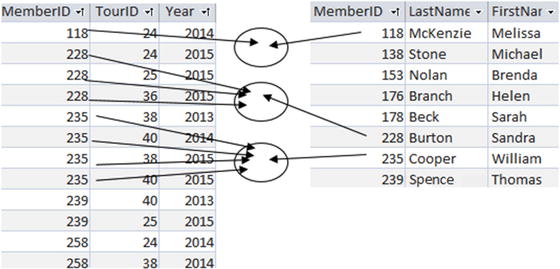
Figure 10-7. Merge join requires each table to be sorted by the field being compared
Sorting tables is an expensive operation. However, if the tables have indexes on the join fields then the rows can be accessed in order by an index scan, making the merge join an option.
Both the merge join and the nested-loops join will be more effective if one or both of the fields in the join condition have indexes.
Different SQL Expressions for Joins
In the previous section I briefly touched on whether the order of the tables in a join would affect the execution. The answer was no for the query in Figure 10-6. However, we have other ways of expressing joins. The two queries that follow have exactly the same execution plans in SQL Server:
SELECT LastName FROM Member m, Entry e WHERE m.MemberID = e.MemberID;SELECT LastName FROM Entry e INNER JOIN Member m ON m.MemberID = e.MemberID;
The following two SQL statements specify the join in terms of nested queries. They have different execution plans from the preceding queries but they are the same as each other:
SELECT LastName FROM Member m WHERE m.memberID IN(SELECT MemberID FROM Entry);SELECT LastName from Member m WHERE EXISTS(SELECT * FROM Entry e WHERE m.MemberID = e.MemberID);
So, should we use or avoid nested queries? The answer, as always, is “it depends.”
Before we compare the preceding two pairs of SQL statements we need to be aware that the output from them is different. The first pair will produce duplicate names (repeating a member’s name for every tournament they have entered). The second pair of queries will produce unique names. To be fair in the comparison we will compare the following two queries, which have identical output:
SELECT DISTINCT LastNameFROM Entry e INNER JOIN Member m ON m.MemberID = e.MemberID;SELECT LastName FROM Member m WHERE m.MemberID IN(SELECT MemberID FROM Entry);
You can see the two plans in Figure 10-8.
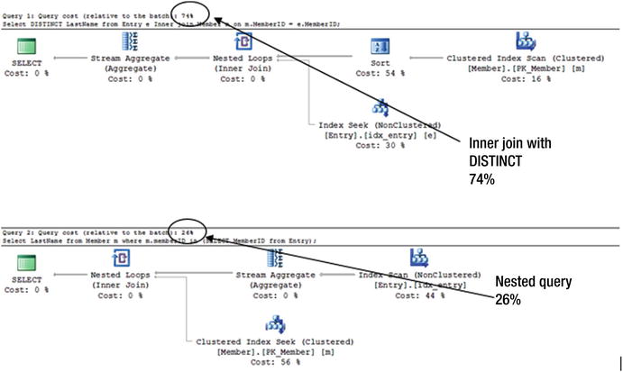
Figure 10-8. The same output but very different execution plans and costs
Figure 10-8 shows the plan for the query using the INNER JOIN keyword at the top and the plan for the nested query underneath. The percentages are saying that if both these queries were executed in one batch then the top one would account for 74 percent of the time and the bottom one 26 percent. That is, the INNER JOIN query takes three times as long as the nested query.
The addition of the DISTINCT keyword in the top query accounts for much of the time. The optimizer has chosen to sort the records in order to prepare to remove the duplicate names. This sorting operation accounts for over half the total cost of the first query. Seeing this plan, you might consider adding an index on LastName so that the records for the Member table could be accessed in LastName order, thus eliminating the need for the time-consuming sort.
Unless you have real insider knowledge, it is just about impossible to second guess what the optimizer will come up with. In the long run it probably doesn’t matter unless the tables have huge numbers of rows or a query is particularly time critical. The important thing to remember is that if you suspect that a critical query is causing a bottleneck, there are tools that can help you understand what is going on. You can then experiment with indexes or the ways the query is expressed to see if that can speed things up.
Summary
Indexes can make a considerable difference in the performance of many queries. However, there is the downside that they have to be maintained. With any tuning of a database it is important to know what the important processes are. There is no point going to any lengths to improve a query that is rarely carried out, and it is counterproductive to improve retrieval performance if most of the time-critical work in your database is the updating of records.
The tools provided by many database systems can provide valuable information. Execution plans can give insight into where the time is being spent in a query. Statistics can be collected about the use of indexes or the distribution of data in a field. All this information is useful when deciding whether the addition of a new index might be worth investigating.
Here are some general rules of thumb for creating indexes.
Primary Key
You need a very good reason not to have an index on the primary key field(s) of a table. Generally a clustered index will be placed on the primary key by default.
Foreign Keys
Joins where the join condition is between a foreign key and a primary key are very common. For this reason an index on foreign keys is usually worth considering.
WHERE Conditions
If you have queries that frequently use particular fields in a WHERE condition, then it is useful to index on those fields. This enables an index seek rather than having to do a table scan to find the relevant rows. This is most useful when the WHERE condition is selective, meaning that it will retrieve only a small subset of the rows.
ORDER BY, GROUP BY, and DISTINCT
Sorting can be a very expensive operation if there are no indexes on the fields involved in the sorting condition. Clearly ORDER BY requires rows to be sorted. Queries that contains DISTINCT or GROUP BY often sort the records to remove duplicates or to aggregate the data. With appropriate indexes, an index scan can be used to retrieve the rows in order, thus eliminating the need for an expensive sorting operation.
Use the Tools
Query optimizers are very sophisticated. They maintain statistics about your tables (number of rows, size of columns, distribution of data, etc.) and use these to help determine an efficient execution plan for a query. If you have a critical query that you want to be as efficient as possible, check the execution plans to see where the time is being spent. You can then experiment with the effects of restating the query or adding additional indexes.