
5
Momentum and Something About Horoscopes
The frictions that prevent efficient markets are numerous.
—JPP
WE’VE SEEN THAT VALUATION IS A KEY BUILDING BLOCK TO forecast returns, but that we must account for other factors. Macro factors give us a lot more context to interpret valuation signals, i.e., what’s priced into markets.
Sentiment also matters. One way to measure sentiment is to look at price momentum. There are many studies on asset price momentum. These studies and my own experience suggest momentum is a useful building block for return forecasting in an asset allocation context, especially when combined with valuation and other signals. However, there are many definitions of momentum. As for the other signals we’ve discussed thus far, we can analyze which definition of momentum works best and in which markets (as long as we don’t overfit our data).
Quantitative investors have long used momentum in their models. In a 2014 Forbes magazine interview with Steve Forbes, Cliff Asness (one of the intellectual giants involved in the CAPE ratio debate we discussed in Chapter 2) talked about the value and momentum signals. When Asness first mentions that momentum works in practice, he says, “Sadly for pure efficient markets guys, good momentum tends to be a good thing in the short-term.”
Asness simply means that “momentum works.” Forbes responds with obvious skepticism: “Sort of the investing equivalent of horoscopes.”
Similar skepticism prevails among many academics and value-oriented investors. For academics who believe in efficient markets, it’s inconceivable that past returns should carry any information about the future. Efficient market theory is frustratingly circular, but the idea is that if its past returns had predictive power, it would be so easy to make money with momentum that investors would pile on these strategies, and opportunities would disappear. So momentum can’t work, because everyone’s doing it. Yet presumably if everyone’s doing it, there must be money to be made; otherwise why do it? Apologies for the geeky spreadsheet analogy, but Excel would reject such a circular reference.
In the same vein, to manage client expectations and legal risks, all pitches for investment products include disclaimers that past returns aren’t indicative of future returns. These disclaimers aren’t only about lack of momentum in asset returns; they also speak to expectations about the persistence of “momentum” (or lack thereof) in investment managers’ skills. (Meanwhile, I have yet to encounter an asset owner who doesn’t consider past performance a major factor in manager selection.)
For value-oriented fundamental investors, the momentum pill is particularly hard to swallow. They tend to distrust momentum strategies. I know several investors who think that to buy something just because it has appreciated in price is perhaps the dumbest thing you can do in investment management: “Why would I buy something because it’s gotten more expensive? It doesn’t make sense!” is something I’ve heard many times. And the same logic applies with negative price momentum: “Why sell something that has gotten cheaper? Something I already thought was a good buy at a higher valuation? I should buy more!”
The key to momentum, however, is not to ignore valuation. It’s to combine it with valuation, as Asness explains in his interview, and as we’ll discuss further. Investors should look for opportunities when both signals agree. For example, buy a cheap asset when its momentum turns positive rather than on the way down, or sell an expensive asset with negative momentum.
Nonetheless, does momentum stand on its own two legs, without an assist from valuation? A lot of research has been published on this topic. In a recent working paper, titled “215 Years of Global Multi-Asset Momentum: 1800–2014,” Christopher C. Geczy and Mikhail Samonov (2015) mention that in 2013, there were approximately 300 papers with the term “momentum” in the SSRN database. Based on their own study, the authors conclude that momentum works at the individual stock level and across asset classes:
We utilize a large amount of historical asset classes to create an out-of-sample test of momentum back to 1800 in country equity indexes, bonds, currencies, commodities, and sectors and stocks. We find that the effect [works] in each asset class, across asset classes, and across momentum portfolios themselves.
They add that “momentum alphas are significant.” The exception seems to be that commodities exhibit mean reversion, i.e., the opposite of momentum. They find that the correlations across momentum strategies have increased drastically in recent years. They suggest that this outcome is driven by the popularity of momentum as an investment style or factor. They warn of “increased strategy risk of overcrowding.”
A Momentum Horse Race
In Chapter 3 we discussed the effectiveness of 3 valuation ratios (P/E, P/B, and P/CF) across 10 equity markets and 6 relative bets between them. We called it a horse race. I mentioned that P/CF won from a market timing perspective, but that P/E won from a relative returns perspective. Does momentum work even better than all three valuation ratios?
The Geczy and Samonov study suggests that positive-momentum assets (“winners”) outperform negative-momentum assets (“losers”) almost everywhere, quite significantly, and out-of-sample. But their study doesn’t cover the same universe of assets and relative bets. My valuation analysis focused on tactical decisions across style, size, and regions, while their momentum study covered individual stocks, equity countries, and equity sectors.
Recently, I ran a study similar to my valuation analysis, but for momentum. My four horses were the trailing six-month, one-year, two-year, and three-year returns. I calculated the correlation between these signals and forward returns at various time horizons. I used the same start date of January 31, 1995, and extended the end date by two months to add recently available data (July 31, 2018).1 Essentially, I replicated what I did in the valuation ratios analysis. Did the momentum signals beat the valuation signals? No, not even close.
For valuation, 97% of the 192 correlations had the expected sign. In contrast, momentum results were all over the place. I calculated correlations between the various trailing windows and one-month, six-month, one-year, two-year, and three-year forward returns. Across absolute and relative bets, I estimated 320 correlations. Only 122 (38%) of them had the expected sign (winners outperform losers). Hence, there was more evidence of mean reversion (losers outperform winners) than momentum.
The main issue appears to be that momentum works better at the one-month horizon than at longer horizons. At the one-month horizon, 66% of the correlations had the correct sign. If I focused on the six-month and one-year lookback windows, which are more commonly used for momentum signals than are two- or three-year windows, the number of correlations with the correct sign went up to 84% (only signals on US small cap stocks did not work in this case). Ultimately, momentum is a shorter-term signal than valuation.
Geczy and Samonov found similar results. They showed that the momentum signal is strongest at the one-month horizon and degrades gradually as the investment horizon gets longer. For stocks, the signal turns into mean reversion roughly around the one-year horizon.
But even at the one-month horizon, the momentum signal was relatively weak, despite high success rates across bets. Average correlation for the best-performing lookback (six months) was only 7% for absolute bets (market timing) and 6% for relative bets. As the lookback expanded, the results got progressively worse. In contrast, we saw in Chapter 3 that valuation signals generated correlations in the 20–40% range.2
Overreaction, or Valuation by Another Name?
An interesting paradox in finance is that as forecasting results get worse and worse, they become better. How does that work? The worst signal possible is one with zero predictability. Signals with strong negative predictability are good, because you can take the other side of the trades. Find the worst investor in the world, an investor who consistently gets it wrong and always loses money, do the opposite, and you’ll be quite successful. (A caveat: The issue in quant finance, however, is that to reverse signals without a theory behind the decision amounts to overfitting/data mining.)
In my momentum study, I found the most predictability—in the form of significant mean reversion—for market timing with three-year lookbacks, applied to a three-year horizon. In other words, asset classes with high three-year returns tend to generate low forward three-year returns, and vice versa. This result could be explained by investor overreaction (De Bondt and Thaler, 1985) or another form of the valuation signal: High three-year momentum asset classes probably have high valuations, and vice versa.
Aside from the observation that a six-month lookback with a one-month forecast horizon worked best, I didn’t find much consistency in my results across relative bets. I did notice that momentum worked consistently at various lookbacks and horizons for one relative bet: emerging markets versus developed markets stocks, a bet for which the valuation signal did not work well. In fact, compared with all other bets, it performed the best on momentum and the worst on valuation—an interesting signal diversification effect. In our tactical asset allocation, perhaps because we focus mostly on valuation, we’ve struggled with this emerging markets versus developed markets decision at times. On a few occasions, we’ve overweighted emerging markets based on valuation—because the asset class looked so cheap—only to get steamrolled by negative momentum. In general, over the last few years, US stocks have continued to outperform stocks in the rest of the world, despite high relative valuation of US stocks.
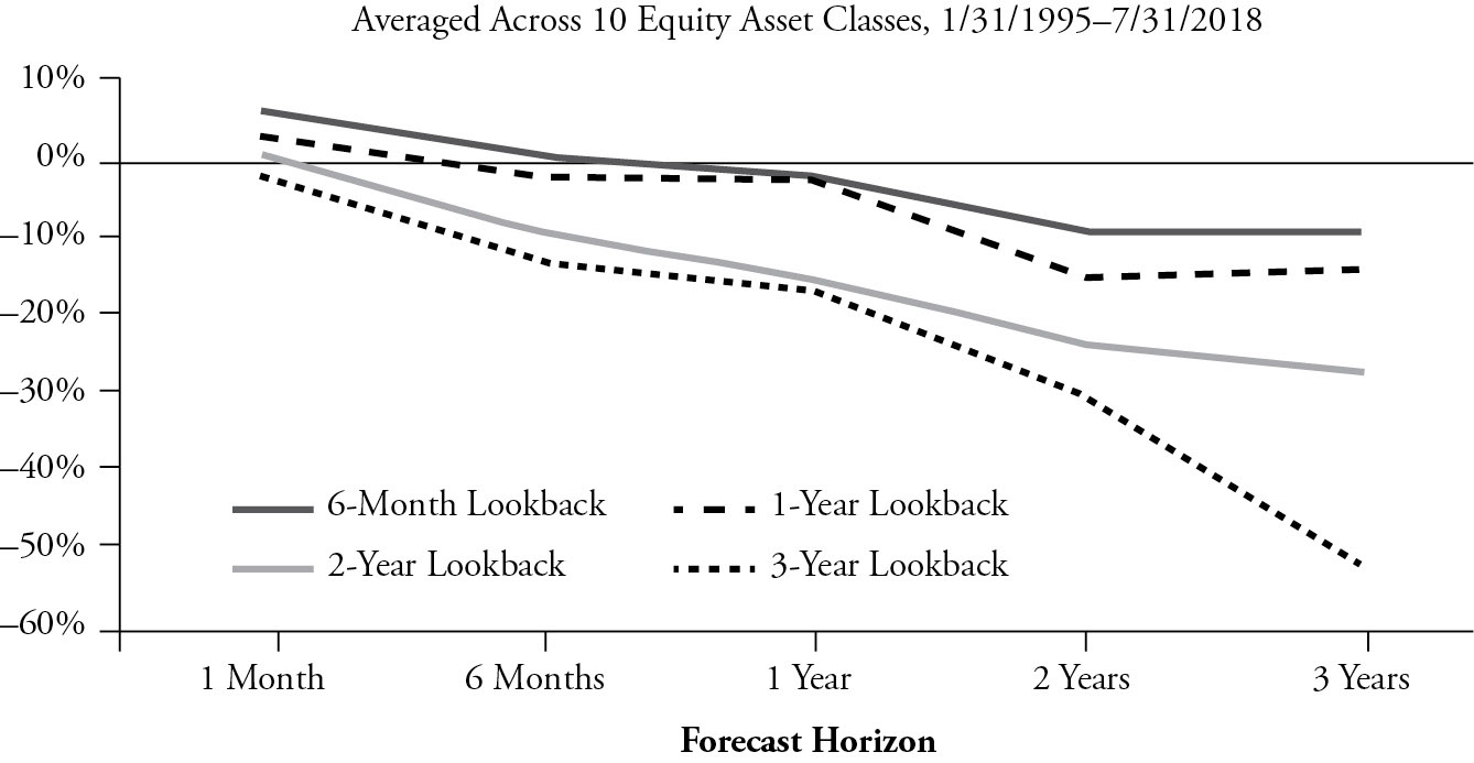
For absolute returns, however, I found a remarkably smooth pattern in my results, as shown in Figure 5.1. This chart shows the average correlation between trailing and forward returns, averaged across the 10 equity asset classes (US small, large, value, and growth; EAFE small, large, value, and growth; world ex-US and emerging markets).3 Any number above the 0% line indicates momentum, while numbers below the line indicate mean reversion. The shorter the lookback window and the shorter the forecast horizon, the more momentum works. The longer the lookback window and the longer the horizon, the more mean reversion works. For these data, there was no exception to this rule of thumb, which I thought was interesting. Figure 5.1 also reiterates clearly that momentum signals were weak, relative to mean reversion/valuation.
FIGURE 5.1 Correlation between trailing returns and forward returns
Some might argue that momentum works better if the most recent month is removed from the data. At the individual stock level, Geczy and Samonov showed that momentum only works if the most recent month is omitted, an adjustment supported by prior studies.4 But to me, this adjustment smells of data mining/overfitting. The authors didn’t find any similar one-month reversal effects for other assets. Hence, I did not drop the most recent month in my momentum analysis. In light of Geczy and Samonov’s results, I doubt it would have made a significant difference in my results.
Bond Momentum: Weak Evidence at Best
In Chapters 1 and 2, we discussed how yield to maturity is a good predictor of future bond returns. I referred to a study by my colleagues Justin Harvey and Aaron Stonacek on absolute bond returns that showed predictive correlations as high as 90%+, depending on the time horizon. Also, I ran a few examples for bond relative returns that revealed some of the best-performing signals I’ve ever found. In general, at the asset class level, valuation works better for bonds than for stocks. But what about bond momentum? Geczy and Samonov find that “although less than other asset classes, momentum is statistically present in government bonds.” They certainly drink the momentum Kool-Aid. Based on my experiments, the evidence of momentum in bond returns is weak, at best.
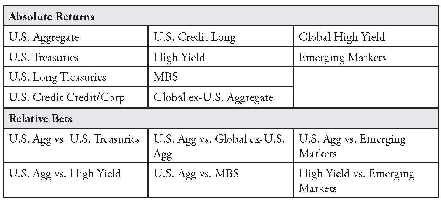
For comparison purposes (and because my spreadsheets were already set up that way), I repeated the same horse race I ran for the equity asset classes, but for bond markets, shown in Table 5.1. I used the same period: January 1995 to May 2018.5 I evaluated the effectiveness of time series momentum with six-month, one-year, two-year, and three-year lookback windows on 10 fixed income asset classes and 6 relative bets between them:
TABLE 5.1 List of Asset Classes and Relative Bets
From a time series/market timing perspective, results on one-month momentum were similar to that for equities: consistently positive across markets, but weak, with predictive correlations—averaged across markets—in the 2–8% range. Unlike for equities, one-month momentum worked well with longer lookback windows (two years and three years). In fact, I found the exact opposite pattern as I did for equities: momentum worked best with long lookback windows (two to three years) and for long predictive horizons (two to three years). With a three-year lookback window and across all predictive horizons, 43 out of the 50 correlations (86%) had the correct sign (compared with 4% for equities). Only high yield and global high yield showed mean reversion.
My take is that interest rates are linked to monetary policy and the business cycle, both of which tend to move incrementally over relatively long periods of time. Spreads also move in a long cycle, but to a lesser extent, with a shorter mean-reversion effect, as evidenced by my results for high yield.
As for relative fixed income bets, momentum did not work at all. It worked so consistently badly that I would qualify these results as “good”: they show meaningful evidence of mean reversion in relative yields. Across bets, lookback windows, and horizons, only 21 out of 120 correlations showed momentum (17.5%), and there was no clear pattern.6
Another way to interpret the result that 17.5% of the correlations showed momentum is that 82.5% of the correlations showed mean reversion. This result agrees with my earlier observation that relative valuations (relative yields) are remarkably predictive in fixed income markets. For this momentum/mean-reversion study, my analysis showed that, as is often the case across markets, the longer the lookback window and the time horizon, the stronger the mean reversion.
To summarize some of the key takeaways on momentum, my view is that it works well when combined with valuation in equity markets. But in fixed income markets, if the objective is to invest across markets with a 6–18-month horizon, investors should focus on mean reversion.
Real-Life Example of Mean Reversion and Valuation and How We Put It All Together
In our Asset Allocation Committee, we use mean reversion in yields and spreads to guide several of our investment decisions. To illustrate with a real-life example, here I show my notes from a meeting in August 2018 when we decided to overweight emerging markets bonds based on valuation. These notes also offer a window into how we look at fundamentals such as aggregate profit margins, and how despite screaming “buy” valuation signals—in this example on US value versus growth—sometimes we hesitate to overweight an asset class if macro and fundamental signals disagree.
The bottom line is that, so far, we’ve discussed valuation, macro, and momentum factors mostly in isolation. But in practice, as these notes illustrate, investors must put it all together, with a heavy dose of experience, judgment, and intuition. (My old quant mindset just rolled over in its grave.)
“Extreme”
Sébastien Page, Notes from Asset Allocation Committee Meeting
The book we use to support our decisions in the Asset Allocation Committee is massive. It contains 180 pages of valuation data, macro signals, fundamentals, and risk analytics.
For each asset class, we get up-to-date levels and percentiles on important indicators. We also get estimates of each indicator’s correlation with forward 12-month returns. If an indicator has high historical effectiveness, we pay more attention to it.
This month, I asked David Clewell and Chris Faulkner-MacDonagh, “Out of the 97 fundamental signals that are in the AAC book, what would be the top 3 trade ideas/signals?”
By trade “ideas” I didn’t mean actual recommendations, because fundamental signals are only part of the puzzle. We explicitly excluded valuation and macro signals from this exercise.
To answer this question, we established the following criteria:
1. Identify the most “extreme” of all the fundamental signals from our AAC book.
2. Rank by R-squared (predictive correlation on forward 12M returns).
3. Pick top 3 most extreme signals with high predictive correlation.
The following top 3 signals surfaced:
Net bank tightening is bullish on stocks vs. high yield bonds (10th percentile over 10 years). Historically, net bank tightening has had a 44% correlation with the forward relative returns on stocks vs. high yield. Valuation metrics also indicate that stocks are cheap relative to high yield (39th percentile), and momentum has been positive for stocks over the last 12 months.
This trade has several risks. In general, in most market environments, it’s a net risk-on position, despite the short high yield leg (unless we scale it to be risk-neutral).
Also:
1. A localized equity volatility shock as we saw in February, with limited spillover to high yield, would work against the trade.
2. There’s a risk that earnings growth remains positive (limited change in high yield default risk) but misses expectations, which would be bad for stocks.
3. Regarding oil prices, energy companies tend to be priced on the long end of the curve, while spot/short-end oil prices affect cash flows and impact high yield spreads more directly. Hence, higher spot prices while the long end remains depressed would work against the trade.
4. Last, in a sideways market with limited risk appetite but no sell-off, high yield can outperform just on the basis of carry.
Verdict: At this point in the cycle, the committee will not add to stocks. And we already have a large underweight position to high yield.
The 7-year real yield differential between Treasuries and bonds is bullish on the USD. It’s at an extreme (99th percentile over 10 years). This signal has a 48% correlation with forward USD appreciation. To benefit from potential USD appreciation, we could move assets back from non-US into US equities (as much as 40% of the risk in this bet is driven by currencies). However, while 12-month momentum is positive, US equity valuations are high relative to non-US equities (92nd percentile over 10 years).
The risks to USD appreciation and a long position in US vs. non-US equities include:
1. A change (toward a more dovish policy) in the path or rate hikes when the 2021 dots are published in September.
2. An unexpected shift in growth differentials, as earlier-cycle economies pick up relative to the US.
3. Earnings disappointments (in the face of high expectations) in the US despite global risk-on sentiment, which could lead to a narrowing of the valuation gap.
4. US debt and deficits lead to a loss of market confidence in the USD as reserve currency.
Verdict: Several committee members have a bullish view on the USD, but we decided not to add to richly valued US stocks.
EBIDTA margins for EAFE value are near an all-time low relative to EAFE growth (12th percentile over 10 years)—a bullish signal for EAFE value. Historically, relative margins revert to a mean—like trees, they don’t grow to the sky. This signal has a 52% correlation with forward returns for EAFE value relative to EAFE growth. The valuation signal for EAFE value is also extremely bullish (first percentile over 10 years). However, momentum is negative, and this trade is perhaps the riskiest of the three, in particular because EAFE value loads heavily on European banks:
1. The European banking sector is at risk of continued low net interest margins, increasingly riskier loans, and a dollar funding squeeze.
2. The ECB could extend its policy of negative interest rates, which could lead to a Japan scenario for banks, according to which they would struggle to maintain profitability due to a flat yield curve.
3. A slowdown in global growth appears to be on the way, which would continue to favor growth stocks over cyclicals.
4. A small number of European banks have significant exposure to USD-denominated Turkey debt.
This analysis led to a broader discussion on extreme relative valuations. Throughout the world, value looks cheap relative to growth stocks. The spreads are at an extreme by historical standards. Similarly, international stocks look cheap relative to the US stocks.
But first, we started with the key question of the day in terms of extreme valuation: Turkey, and EM debt in general.
EM DEBT (USD) ATTRACTIVE ON VALUATION
“In fixed income markets, there’s strong mean reversion (barring defaults). Unlike in equities, you get your money back—the terminal value is known!” said one committee member. Our dashboards in the AAC book support this statement: our strongest valuation signals are the relative YTMs on various fixed income asset classes. The terminology I often heard at my previous employer was that when the bonds are “money-good,” you have “stored alpha.”
The fixed income team has issued a high conviction rating on EM debt, on valuation. Relative to other risk assets in fixed income, EM debt looks cheap. For example, its ratio to high yield (on a spread basis) is near an all-time high.
The “house view,” to the extent we have one, is that despite ugly headlines, it’s not the first time Turkey has faced a crisis, and the current situation is unlikely to pose a systemic risk. Also, emerging markets have changed since the 1990s, with a stronger middle class, FX reserves, fewer cyclical companies, more technology companies, etc. Therefore, we will evaluate liquidity conditions and move from an underweight –50-bps to an overweight +50-bps position in EM debt. We will fund this move from TIPS (we don’t see major inflation pressure in the short run).
Doing so will increase our risk at the portfolio level, but as discussed before, we’ve already derisked our portfolios substantially.
To emphasize: We haven’t changed our defensive, risk-off stance. This move is a valuation play, as we see this “extreme” valuation as a tactical opportunity.
GROWTH VS. VALUE AT AN EXTREME
Another extreme signal is how cheap value looks relative to growth. One committee member pointed to a dashboard from our book and asked the provocative question: “What will it take for us to decide to overweight value?” On the dashboard in question, 21 indicators flash bright red against growth and in favor of value. Eight of them are in the 99th percentile and above.
It’s a puzzle to most committee members why value hasn’t outperformed this year, in the face of cheap valuations, higher rates, a cyclical upswing in growth and earnings, and higher energy prices. The key issue might be that no one wants to overweight value this late in the cycle. Also, technology disruption plays a role. “A lot of value isn’t value,” said one committee member.
To which another member added: “18% of companies in the S&P 500 face secular risks. A majority of these companies are in the value sector.”
Also, financials are the cheapest sector in the US market, but they could still take a hit in a mild recession. Meanwhile, it’s hard to imagine Google’s earnings going down –50%. A broader, related question, which will be discussed in an upcoming macro call, is the following: Which sector would provide protection should we face a recession? History might not be a good guide to answer this question—we must consider the current environment.
On the other hand, in favor of value, growth feels concentrated. Large technology platform companies have grown at an accelerated pace, which, mathematically, can’t be sustainable, unless they eventually engulf the entire economy. And if we get a trade deal with China, we could see a value rally (energy, financials), perhaps of similar magnitude as when Trump got elected.
Takeaway: As in several of our previous meetings, we had a good debate on the value vs. growth question but decided to stay at neutral.
To conclude, this month we looked at extremes in fundamentals and relative valuations. We think EM debt presents a good opportunity. And we’ve derisked our portfolios enough that we feel comfortable playing some offense. Also, we recognize that value is extremely cheap relative to growth, but in the US market we will hold at neutral for now, given the late-cycle environment and our secular preference for growth.
Notes
1. EAFE large versus small tests start on January 31, 1998. Everything else, including EAFE large and EAFE small as individual assets, starts on January 31, 1995. Data source: Bloomberg Finance L.P. Field: TOT_RETURN_INDEX_GROSS.
2. Here I’m reversing the sign for comparison with the momentum signal. Again, this is just a convention related to how the signals are interpreted.
3. EAFE large versus small tests start on January 31, 1998. Everything else, including EAFE large and EAFE small as individual assets, starts on January 31, 1995. Data source: Bloomberg Finance L.P. Field: TOT_RETURN_INDEX_GROSS.
4. See Jegadeesh and Titman (1993), for example.
5. Bloomberg Barclays. Data series: U.S. Aggregate (LBUSTRUU Index), U.S. Corporate (LUACTRUU Index), U.S. High Yield (LF98TRUU Index), Emerging Markets (EMUSTRUU Index), Global ex-U.S. Aggregate (LG38TRUU Index), U.S. MBS (LUMSTRUU Index), U.S. Treasuries (LUATTRUU Index), U.S. Long Credit (LULCTRUU Index), U.S. Long Treasury (LUTLTRUU Index), Global High Yield (LG30TRUU Index).
6. Except that six-month and one-year lookbacks with one-month predictive horizon seemed to work with some consistency, albeit weakly—a result in line with equities and Geczy and Samonov’s paper.