7
Risk-Based Investing and Something About Sailboats
Markets are only partially efficient.
—JPP
IN MAY 2016, I NEEDED IDEAS FOR A PRESENTATION AT THE 69th CFA Institute Annual Conference, held in Montreal. I’m French Canadian, so this was an especially exciting opportunity. My colleague Stefan Hubrich suggested research that he and colleagues (Bob Harlow, Anna Dreyer, and others) had done to capitalize on the short-term predictability in volatility. He mentioned that managed volatility and covered call writing are two of the few systematic investment approaches that have been shown to perform well across a variety of empirical studies. Moreover, they work well in practice (we manage such strategies as overlays or components of multi-asset portfolios). Stefan added: “So far, these two strategies have been studied separately, as stand-alone approaches. But it turns out that they’re negatively correlated. When combined, they create a powerful toolset for portfolio enhancements.”
Stefan, Bob, Anna, and other colleagues (David Clewell, Charles Shriver, and Toby Thompson) helped me prepare the presentation. Stefan, Bob, Anna, and I (2016) also published a paper for the conference proceedings, titled “Return of the Quants: Risk-Based Investing.”
In Montreal, after a quick introduction in French, I switched to English. (While I speak French with family, I’ve lost track of how to translate technical finance terms from English to French.) I worried that terms like “fat tails” may sound odd in French.
I began my presentation with the observation that the financial services industry seems obsessed with return forecasting. Asset owners, investment managers, sell-side strategists, and financial media pundits all invest considerable time and resources to predict the direction of markets. Even so, I argued, risk-based investing may provide easier and more robust ways to improve portfolio performance, often without the need to forecast returns directly.
To emphasize the importance of risk-based investing, I showed that since 2000, volatility has increased significantly. In the 1940s, on average, there were four days per year during which stocks moved by three standard deviations or more (“three-sigma days”). The Second World War created a lot of this turbulence. In the six decades that followed, the average rose no higher than three days per year. But between 2000 and 2010, on average there were nine three-sigma days per year—more than any time in the preceding 80 years.1
Based on the normal distribution, a three-sigma day should occur only 0.6 time per year (on average). We often refer to extreme returns as “tail events” because they lie in the tails of the probability distribution. Clearly, the tails have gotten fatter in the markets, and the normal distribution may not be a reliable tool to measure investment risk.
I offered the audience several plausible explanations for this increase in market turbulence. Some of the usual suspects include central bank interventions, global market integration, high-frequency trading, and increased use of derivatives and structured products.
Whatever the root cause, I insisted that investors must manage exposure to large and sudden losses. And to do so, they must recognize that volatility—and thereby exposure to loss—is not stable through time. I showed that from 1994 to 2016, the rolling one-year standard deviation for a 60/40 portfolio (60% stocks, 40% bonds) ranged from a low of less than 5% to a high of 20%. This portfolio’s rolling three-year standard deviation over the same period ranged from about 5% to about 15%.2
This example made it clear that a constant (fixed weight) asset allocation does not deliver a constant risk exposure. To a certain extent, it invalidates most financial planning advice. Is a 60/40 portfolio appropriate for a relatively risk-averse investor? The answer depends on the volatility regime. In some relatively calm environments, a 60/40 portfolio may deliver 5% volatility, which seems appropriate for a conservative investor. However, in turbulent markets, the same portfolio may deliver as much as 20% volatility, which seems more appropriate for an aggressive investor, with a thick skin and high risk tolerance. What’s the solution? Is there a way to stabilize a portfolio’s risk exposure over time?
Managed Volatility Backtests
The managed volatility strategy is designed for that purpose. It relies on the short-term predictability in volatility. In a nutshell, the strategy adjusts the asset mix over time to stabilize a portfolio’s risk. For example, we may adjust a 60/40 portfolio’s exposure to stocks all the way down to 20% when markets are volatile and all the way up to 75% when markets are stable. The asset mix becomes dynamic, but portfolio volatility is stabilized. As an analogy, think of how a sailor must dynamically adjust the sailboat’s sails to adapt to wind conditions and keep a straight line. The strategy is portable and can easily be applied as a futures overlay to smooth the ride for almost any portfolio.3 Importantly, it has been thoroughly backtested. In Table 7.1, I summarize a sample of 11 studies on the topic.4
TABLE 7.1 Prior Studies on Managed Volatility
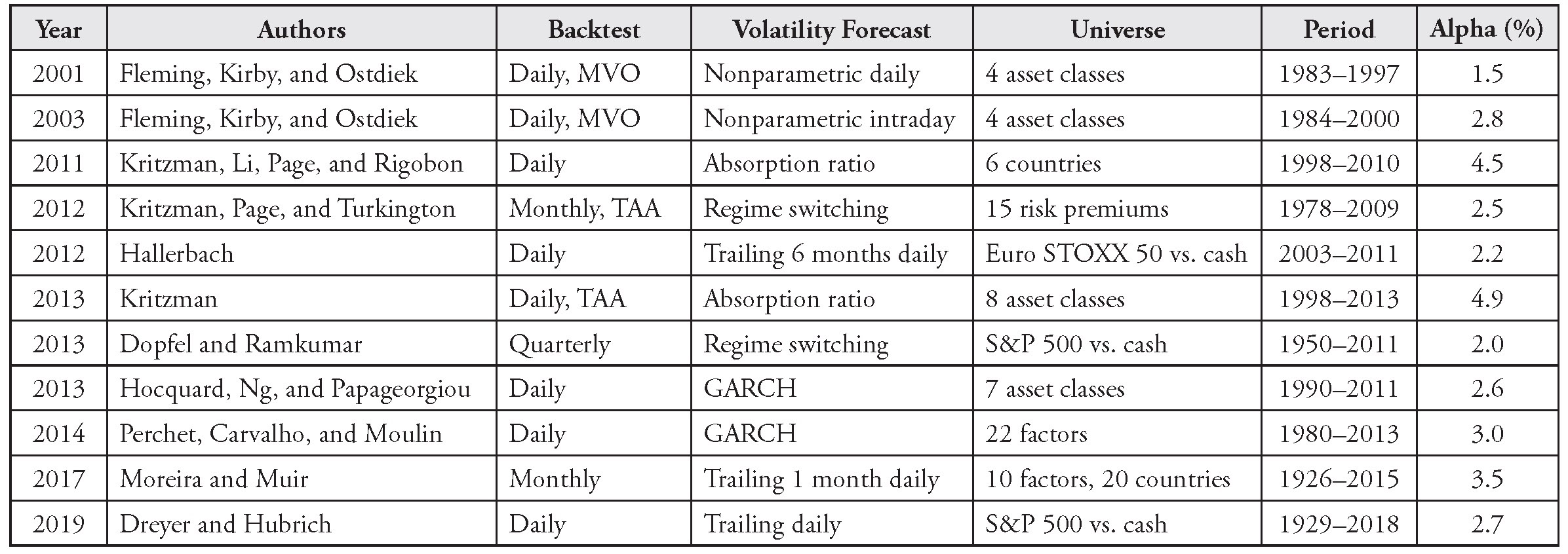
To compare results across studies, I report alpha over volatility-matched, buy-and-hold benchmarks. Another way to think about these results is that for the same return, managed volatility portfolios delivered less volatility (and, it is hoped, less exposure to loss) than did their buy-and-hold benchmarks. When the authors did not report these results directly, I scaled Sharpe ratios to match the volatility of the static benchmark.
The results are encouraging, especially in a low-rate environment in which expected returns are depressed across stocks and bonds. Managed volatility seems to improve performance across studies. Indeed, the strategy appears to work well across risk forecast methodologies, asset classes (stocks, bonds, currencies), factors/risk premiums, regions, and time periods. These results suggest that any asset allocation process can be improved if we incorporate volatility forecasts.
But a few caveats apply. Cynics may argue that only backtests that generate interesting results get published (earlier I mentioned publication bias). Authors often make unrealistic assumptions about implementation. For example, they assume portfolio managers can rebalance everything at the closing price of the same day the signal is generated. Worse, some ignore transaction costs altogether. And a more subtle but key caveat is that some strategies do not use budget constraints, such that part of the alpha may come from a systematically long exposure to equity, duration, or other risk premiums versus the static benchmark.
Though these risk-adjusted alphas should be shaved to account for the inevitable implementation shortfall between backtests and reality, managed volatility has been shown in practice to reduce exposure to loss and smooth the ride for investors, at a very low—or even positive—cost in terms of returns. Dreyer and Hubrich (2019) treat cost and implementation carefully, because they are rooted in live portfolio experience.
Consider a backtest our team built specifically to represent real-world implementation, based on data from January 1996 to December 2014. For this example, we set a target of 11% volatility for a balanced portfolio of 65% stocks and 35% bonds. We scaled the overlay to avoid any systematically long equity or duration (i.e., bond) exposure versus the underlying portfolio—consequently, the strategy is expected to keep a risk profile similar to a 65/35 exposure on average. We allowed the managed volatility overlay to reduce equity exposure to as low as 20% and increase it as high as 75%.5
We then applied a band of 14% and 10% volatility around the target. As long as volatility remained within the band, no rebalancing was required. When volatility rose above or fell below the bands, the strategy rebalanced the overlay to meet the (expected) volatility target. We used a wider upper band because volatility tends to spike up more than it spikes down, so these asymmetrical bands were meant to reduce noise and minimize the intrusiveness of the algorithm.
Within the portfolio, we assumed that 95% of assets were invested directly in a balanced strategy composed of actively managed mandates (i.e., within each of the asset classes, managers selected securities).6 The remaining 5% were set aside as the cash collateral for the volatility management overlay, which we assumed was invested in Treasury bills. When volatility was at target, the futures overlay was set to match the balanced portfolio at 65% stocks and 35% bonds. Equity futures were allocated 70% to the S&P 500 and 30% to the MSCI EAFE (Europe, Australasia, and the Far East) Index futures, to reflect the neutral US/non-US equity mix inside the balanced strategy. Last, we imposed a minimum daily trade size of 1% and maximum trade size of 10% of the portfolio’s notional.
To forecast volatility, we used a DCC–EGARCH model (dynamic conditional correlation—exponentially weighted generalized autoregressive conditional heteroscedasticity) with fat-tailed distributions. This model closely replicates the implied volatility on traded options and thus how investors in general forecast volatility. DCC accounts for time-varying correlations. The ARCH model, as I mentioned, accounts for the time series properties of volatility, such as its persistence or tendency to cluster. We reestimated the model daily using 10 years of data ending the day prior to the forecast.7 Volatility forecasts were updated daily using the most current parameter estimates. Importantly, we strictly used information known at the time to determine how to trade the overlay.
As expected, over the 18-year period studied, managed volatility consistently stabilized volatility compared with its static benchmark. The algorithm worked particularly well during the 2008–2009 financial crisis. The strategy was quite tactical. Although it did not trade more than 10% of the portfolio’s notional value in futures in a given day, some of the shifts in equity allocations were meaningful and occurred over relatively short periods of time.
In this example, active managers added returns over passive benchmarks (after fees) in the underlying building blocks through security selection. They slightly increased exposure to loss. When we applied the managed volatility overlay to this portfolio, we sacrificed a few basis points of returns, but we reduced drawdown exposure. Because we avoided large equity exposures throughout the high-volatility regimes, the historical maximum drawdown was 10% lower than for a static benchmark.
Over the last two years, we have managed such strategies for an insurance company and other clients. As we manage through the equity sell-off of 2020, so far these strategies have performed well.
Why would managed volatility improve risk-adjusted returns? To explain this success, we must understand why volatility is persistent (and therefore predictable). Periods of low and high volatility—risk regimes—tend to persist for a while. This persistence is crucial to the success of the strategy, and it means that simple volatility forecasts can be used to adjust risk exposures. A fundamental argument could be made that shocks to the business cycle themselves tend to cluster. Bad news often follows bad news. The use of leverage—in financial markets and in the broader economy—may also contribute to volatility clustering. Leverage often takes time to unwind. Other explanations may be related to behavioral aspects of investing that are common to investors across markets, such as “fear contagion,” extrapolation biases, and the financial media’s overall negativity bias.
In terms of managing tail risk specifically, one way to explain how managed volatility works is to represent portfolio returns as a “mixture of distributions,” which is related to the concept of risk regimes. When we mix high-volatility and low-volatility distributions and randomly draw from either, we get a fat-tailed distribution. By adjusting risk exposures, managed volatility essentially “normalizes” portfolio returns to one single distribution and thereby significantly reduces tail risk.
Short-term expected (or “forward”) returns do not seem to increase after volatility spikes, which explains why managed volatility often outperforms buy and hold in terms of the Sharpe ratio (or risk-adjusted performance in general).
This phenomenon has been studied in academia (see the article published in the Journal of Finance titled “Volatility Managed Portfolios,” by Alan Moreira and Tyler Muir, 2017). Most explanations focus on the time horizon mismatch between managed volatility and value investing. Moreira and Muir observe that expected returns adjust more slowly than volatility. Therefore, managed volatility strategies may re-risk the portfolio when market turbulence has subsided and still capture the upside from attractive valuations. The performance of managed volatility around the 2008 crisis is a good example. As Moreira and Muir put it:
Our [managed volatility] portfolios reduce risk taking during these bad times—times when the common advice is to increase or hold risk taking constant. For example, in the aftermath of the sharp price declines in the fall of 2008, it was a widely held view that those that reduced positions in equities were missing a once-in-a-generation buying opportunity. Yet our strategy cashed out almost completely and returned to the market only as the spike in volatility receded. . . . Our simple strategy turned out to work well throughout several crisis episodes, including the Great Depression, the Great Recession, and the 1987 stock market crash.
Stefan Hubrich points out that there is another way to think about how managed volatility may increase Sharpe ratios in certain market environments: think of time diversification as similar to cross-asset diversification. Suppose we invest in five different stocks with the same Sharpe ratios but very different volatility levels. If we assume the stocks are uncorrelated, we should allocate equal risk (not equal value weights) to get the Sharpe ratio–maximizing portfolio. The same logic applies through time; the realized variance of the portfolio is basically the sum of the point-in-time variances. To get the highest Sharpe ratio through time, we should allocate equal risk to each period.
However, managed volatility does not always outperform static portfolios. For example, when spikes in volatility are followed by short-term return gains, managed volatility may miss out on those gains (versus a buy-and-hold portfolio). Also, it is possible for large market drawdowns to occur when volatility is very low. In those situations, managed volatility strategies that overweight stocks in quiet times (to a higher weight than the static portfolio) may underperform.
In sum, the empirical observations in support of managed volatility—volatility persistence and the lack of correlation between volatility spikes and short-term forward returns—hold on average, but not in all market environments. Ultimately, volatility is forecastable because it “clusters”; hence, managed volatility stabilizes realized volatility and reduces tail risk. It also improves risk-adjusted returns due to a “time diversification” between risk regimes, as well as the empirical reality that risk-adjusted equity market returns are not higher when volatility is high. (Absolute expected returns are higher in high-volatility periods, but not enough to compensate for the higher volatility.) It’s possible that managed volatility can “sell low” into a bear market and lose ground, but it is also often “long risk” during expansions. Throughout the cycle, it may provide higher exposure to the equity risk premium than would a typical long-only fund without additional risk.
For more on this topic, as well as a robust empirical study and a fascinating discussion on how to think about managed volatility, see Dreyer and Hubrich (2019). To quote Stefan Hubrich, one of the authors of this paper:
Managed volatility can have high tracking error to the underlying for extended (multi-year) periods, if it’s scaled large enough so that it can make a difference. It’s a fundamentally different strategic, very long-term asset allocation—rather than an “active” strategy benchmarked to the underlying that can be evaluated quarterly. Warren Buffet once said that if the internet had been invented first, we wouldn’t have newspapers. I tend to believe that if managed volatility had been invented first, we might not have as many traditional balanced funds. It’s really the more appropriate long term/unconditional way to invest, as the portfolio is always—each day—aligned with your risk tolerance.
Covered Call Writing (Volatility Risk Premium)
While managed volatility is used mostly to reduce exposure to loss, we can think of covered call writing as the other side of the coin for risk-based investing, in that investors use it mostly to generate excess returns. The basics of the strategy are simple: the investor sells a call option and simultaneously buys the underlying security or index. Covered call writing gives exposure to the volatility risk premium, one of the “alternative betas” that have risen in popularity recently.
The strategy relies on the predictability in the difference between implied volatility (embedded in options prices) and realized market volatility. Historically, implied volatility has almost always been higher than subsequent realized volatility. Hence, when appropriately hedged, the strategy sells implied volatility and buys realized volatility, without any (or with very little) direct market exposure. As mentioned by Roni Israelov and Lars N. Nielsen in “Covered Call Strategies: One Fact and Eight Myths” (2014), “The volatility risk premium, which is absent from most investors’ portfolios, has had more than double the risk-adjusted returns (Sharpe ratio) of the equity risk premium.”
In Table 7.2, I show results from several empirical studies on the performance of covered call writing.8 The strategy has generated (simulated) alpha across markets and time periods and for several variations of the methodology. William Fallon, James Park, and Danny Yu, in their 2015 paper “Asset Allocation Implications of the Global Volatility Premium,” backtest volatility risk premium strategies across 11 equity markets, 10 commodities, 9 currencies, and 4 government bond markets. They find that “the volatility risk premium is sizable and significant, both statistically and economically.”
TABLE 7.2 Prior Studies on the Volatility Risk Premium

The same caveats apply as for the managed volatility studies—namely, that only backtests with good results tend to get published and that authors often ignore implementation shortfall between backtests and realized performance. Nonetheless, in practice, covered call writing has been shown to deliver good risk-adjusted performance, although perhaps not as high as 6–7% alpha across all market regimes.
As we did for managed volatility, we must ask why we should expect the volatility risk premium to continue to perform well going forward. What are the theoretical foundations behind the strategy? First, there’s demand for hedging. For example, insurance companies need to hedge explicit liabilities they have written. Generally, investors in many countries are increasingly seeking drawdown protection. By selling options, investors should earn a risk premium. The magnitude of this premium is determined by the supply and demand imbalance for insurance.
Some observers may say that covered call writing does not sell protection. But if the puts are overpriced because of the demand for protection, calls should be overpriced as well, through put-call parity. Indeed, dealers can replicate the put with the call and a short forward position. As long as no arbitrage occurs, demand for protection will also drive up the call price.
The history of implied volatility for US stocks is consistent with the fact that investors crave protection. Historically, implied volatility was almost always higher than realized volatility. This spread loosely explains the performance of covered call writing.
Second, beyond the “demand for hedging” theory, a simpler explanation for the volatility risk premium has been proposed: it may simply represent compensation for its tail risk. Selling volatility generates long series of relatively small gains, followed by infrequent but large losses. (In statistical terms, returns are said to exhibit negative skewness and excess kurtosis. We’ll define these terms in more detail in Chapter 8.) In 2008, for example, realized one-month volatility on the S&P 500 shot up significantly above implied volatility, and covered call writing strategies experienced significant losses. Fallon, Park, and Yu report similar tail risks in the volatility risk premium for 33 out of 34 of the asset classes they studied.
Both explanations—the demand for hedging and the compensation for tail risk—are, in fact, connected. Insurance providers should expect negatively skewed returns, by definition. The bottom line is that if long-term investors can accept negative skewness in their returns, they should get compensation through the volatility risk premium.
A Powerful Combo of Risk-Based Strategies
Investors can use managed volatility to reduce the tail-risk exposure in covered call writing. The idea is to think of risk-based strategies as a set of tools, rather than stand-alone approaches. Low or even negative correlations between risk-based strategies can add a lot of value to a portfolio, even when the individual strategies’ Sharpe ratios are relatively low.
In my presentation at the CFA Institute Annual Conference, I used data from a study by my colleague Stefan Hubrich to show that the correlation of monthly returns above cash from January 1996 to December 2015 between covered call writing and managed volatility (overlay only, without the equity exposure) was –20%.9 This result suggests that when investors incur a loss on covered call writing, they are likely to have already de-risked their portfolio with their managed volatility overlay, thus reducing the impact of the loss.
To further illustrate the power of diversification between covered call writing and managed volatility, Stefan estimated returns, volatilities, downside risk, and relative performance statistics for the stand-alone and combined strategies. Based on data from January 1996 to December 2015, the risk-return ratio of the S&P 500 is 0.41. When combined with the covered call writing strategy (with gross exposure capped at 125%), the S&P 500’s risk-return ratio increases from 0.41 to 0.49, while downside risk is only marginally reduced. But when we add managed volatility, the risk-return ratio jumps from 0.49 to 0.69 (even though the stand-alone managed volatility strategy had a relatively low risk-return ratio of 0.17), and downside risk is reduced substantially.
Takeaways and Q&A
To summarize, volatility has been shown to be persistent, and in the short run, it has not been predictive of returns. Accordingly, managed volatility is one of the few systematic investment strategies that historically outperformed buy-and-hold benchmarks across a wide range of markets and data samples.
Covered call writing is another systematic strategy that has been shown to generate attractive risk-adjusted performance across many empirical studies and in practice. The strategy gives access to the volatility risk premium, which pays those who provide insurance and assume the associated tail risk.
Combining managed volatility and covered call writing can be extremely effective, because these two strategies are negatively correlated and can easily be added to conventional portfolios. And despite our industry’s obsession with return forecasting, these two investment strategies focus on risk. They do not require bold predictions on the direction of markets.
Q&A
The large conference audience asked interesting questions, and I hope I offered insightful replies. What follows is an edited version of that conversation.
Q: How is managed volatility different from risk parity?
A: Risk parity seeks to equalize risk contributions from individual portfolio components. Usually, it is applied at the asset class level and assumes that Sharpe ratios are all the same across asset classes and that all correlations are identical. Low-volatility asset classes, such as bonds, are typically levered up to increase their risk contribution to the portfolio. On the surface, therefore, it is quite different. It is a way to allocate the portfolio that doesn’t address risk disparity through time. (It’s a fact that periods of high volatility with high exposure to loss alternate with periods of lower volatility.)
However, some risk parity strategies maintain a target volatility for the entire portfolio. In a sense, this means that there can be an implied managed volatility component to risk parity investing.
Still, to believe in risk parity investing, you must believe that Sharpe ratios are the same in all markets and under all market conditions, which I believe is not always the case.
Q: Why not just focus on downside volatility?
A: Downside volatility can be calculated in many ways. For example, you can isolate deviations below the mean to calculate semistandard deviation, or you can use conditional value at risk (average loss during extreme downside markets) and try to manage risk at that level. The volatility surface from option prices, for example, embeds implicit estimates of the tail of the distribution.
To focus on downside risk makes sense. Is there such a thing as upside risk? In general, though, it is more difficult to forecast the directionality of volatility than volatility itself. Doing so in managed volatility backtests may not change the forecast that much. We’ll discuss downside risk forecasts in more detail in the next chapter.
Q: The volatility risk premium has negatively skewed returns. Could you expand on the implications?
A: Indeed, the volatility risk premium does not have a symmetrical payoff. The purpose of the strategy is to earn the premium from the difference between implied and realized volatility. Most of the time, you make a small gain. But when those volatilities cross, relatively large losses occur. That is one of the reasons for the risk premium. If you are a long-term investor and you accept this asymmetry, you should expect to be compensated for it.
Q: Is there a risk of buying high and selling low with managed volatility? And how does managed volatility relate to a value-based approach?
A: This question comes up often around managed volatility. The goal is to lower exposure to the market on the way down and get back in when volatility goes back down but when valuations are still attractive. Moreira and Muir (2017) have run a set of tests related to this question. They argue that time horizon matters. Across more than 20 different markets and risk premiums, they show that the correlation between this month’s volatility, calculated very simply on daily data, and next month’s volatility is about 60%, which indicates persistence in volatility.10
Then they examined the correlation between volatility this month and returns next month. They found a 0% correlation. If it were negative, it would work even better, but the 0% correlation is good enough to substantially improve risk-adjusted returns through adjustments of risk exposures based on volatility.
The intuition is that value-focused investors try to buy low and sell high, but they typically do so with a longer time horizon. Often, they wait for market turbulence to subside before they buy low. In fact, valuation signals don’t work very well below a 1-year horizon, and they tend to work best when the horizon is relatively long: 5 to 10 years.
The difference in time horizon between a managed volatility process with a one-month horizon and a longer-cycle valuation process often allows managed volatility investors to get back into risk assets at attractive valuations.
Moreira and Muir’s study (2017) is particularly interesting because they tested several market crises, including the crash of 1987, and the strategy with a one-month volatility forecast outperformed buy and hold over all crisis periods.
Q: Do liquidity issues arise when you implement managed volatility and covered call writing strategies for very big funds?
A: You can run managed volatility with very liquid contracts, such as S&P 500 and Treasury futures. If the portfolio is not invested in such plain- vanilla asset classes, there might be a trade-off between basis risk (how well the futures overlay represents the underlying portfolio) and liquidity, but this trade-off can be managed with a risk factor model and a tracking error minimization optimization. Nonetheless, it’s irrefutable that liquidity risk can create significant gaps in markets, and some investors—for example, insurance companies—buy S&P 500 put options in combination with managed volatility to explicitly hedge this gap risk.
As for covered call writing, index options on the S&P 500 are liquid. However, for other options markets, investors must assess the trade-off between illiquidity and the risk premium earned.
Q: What are the costs of implementing these strategies?
A: The trading costs for a managed volatility overlay are remarkably low because of the deep liquidity of futures markets, perhaps 10–18 bps. If the overlay is not implemented in-house, a management fee of 10–20 bps will be accrued. Accessing the volatility risk premium through options is probably on the order of 40–60 bps for transaction costs plus a management fee. Note that these are just estimates, and costs always depend on the size of the mandate and a variety of other factors.
Q: Can you use managed volatility to inform currency hedging decisions?
A: With currency hedging, investors must manage the trade-off between carry, which is driven by the interest rate differential, and the risk that currencies contribute to the portfolio. Importantly, the investor’s base currency matters. When investors in a country with low interest rates hedge their currency exposures, they typically benefit from risk reduction, but it comes at the cost of negative carry. Japan, for example, has very low interest rates, which means currency hedging is a “negative carry trade.” So it is very hard to convince Japanese investors to hedge, even though from a risk perspective, it may be the right decision.
In Australia, by contrast, currency hedging offers positive carry because local interest rates are relatively high. Australian investors love to hedge their foreign currency exposures back to the home currency. But the Australian dollar tends to be a risk-on currency. Ultimately, investors can use managed volatility to optimize this trade-off dynamically. As volatility goes up, they can adjust their hedge ratios to reduce exposure to carry (thereby reducing their risk-on exposures). To do so, they must recalculate the risk-return trade-offs on an ongoing basis and reexamine the correlations between currencies and the underlying portfolio’s assets, as well as with their liabilities when applicable.
Q: Is it better to do option writing when the Volatility Index (VIX) is high or low?
A: It is generally better to sell options when implied volatility is overpriced relative to expected realized volatility. For example, when investors are nervous over a high-volatility event or a market drawdown, options may be overpriced. The determinant is not necessarily high or low volatility, but rather the effect investor behavior is having on option prices relative to the real economic volatility in the underlying investment. To get the timing right is not easy, of course, but active management may add value over a simple approach that keeps a constant exposure to the volatility risk premium.
Q: With so much money chasing managed volatility, do you think the alpha is likely to become more elusive?
A: It’s true that managed volatility is harder to implement when everyone’s rushing for the door at the same time. And the risk of overcrowding—and associated gap risk—is always there. But managed volatility still works well when we slow down the algorithm.
Also, over time, profit opportunities from “overreaction” should entice value or opportunistic investors to take the other side of managed volatility trades. I think of it as an equilibrium. As managed volatility starts causing “overreaction,” the premium that value buyers can earn if they take the other side of the trade will become more and more attractive. That will entice them to provide liquidity.
Notes
1. Factset, Standard and Poor’s, and T. Rowe Price. Standard deviation is measured over the full sample of data (1940–2015).
2. The balanced strategy is 60% S&P 500 and 40% Barclays U.S. Aggregate Index rebalanced monthly. Sources: Ibbotson Associates, Standard & Poor’s, and Barclays.
3. With an overlay, we trade futures contracts to change broad market exposures in the portfolio. We typically don’t transact in the underlying asset classes, which means the portfolio managers responsible for the various asset class–level mandates aren’t affected. In other words, they are “undisturbed”; i.e., they can manage their portfolio as they normally do, without excessive inflows or outflows or changes to their process.
4. Readers should refer to the original papers for more information on the volatility forecast methodologies. I report the average of key results or the key results as reported by the authors. MVO refers to mean-variance optimization; TAA refers to tactical asset allocation, expressed as various multi-asset portfolio shifts; all other backtests involve timing exposure to a single market or risk premium. Countries refer to country equity markets, except for Perchet, Carvalho, and Moulin (2014), which includes value and momentum factors across 10 countries and 10 currencies. Some backtests in Fleming, Kirby, and Ostdiek (2001) and Perchet, Carvalho, and Moulin (2014) involve shorter time series because of the lack of available data. The backtest by Dopfel and Ramkumar (2013) is in-sample. The regime-switching model in Kritzman, Page, and Turkington (2012) combines turbulence, GDP, and inflation regimes. Regarding transaction costs, Fleming, Kirby, and Ostdiek (2001, 2003) assume execution via futures contracts and estimate transaction costs in the 10–20-bps range. Moreira and Muir (2017) report transaction costs in the 56–183-bps range for physicals. Dreyer and Hubrich (2019) use a 3-bps bid-ask spread for every futures trade, based on the actual trading pattern of the strategy. They show a 10–20% deterioration in results when adding these transaction costs to the simulation. However, they more than recover these costs when they also add caps on trading behavior: they only trade if the proposed trade is >10%, and they only implement up to 50% same day. All other studies do not report transaction costs.
5. The model allows for adding risk above the 65% strategic allocation when volatility is low. In fact, investors can calibrate managed volatility overlays to any desired risk level, including levels above the underlying portfolio’s static exposure.
6. Note that we used an actual track record for an actively managed balanced fund. However, this example is for illustrative purposes only and does not represent performance that any investor actually attained. Model returns have inherent limitations, including assumptions, and may not reflect the impact that material economic and market factors may have had on the decision-making process if client funds were actually managed in the manner shown.
7. We used an expanding window, increasing from 3 years to 10 years, until 10 years of data became available.
8. The BXM Index refers to the CBOE S&P 500 BuyWrite Index. It is a benchmark index designed to track the performance of a hypothetical buy-write (covered call writing) strategy on the S&P 500. Fallon, Park, and Yu’s start dates vary from January 1995 to February 2001 based on data availability, and alpha is averaged across all backtests.
9. All data sources and methodologies from this section are described in “Return of the Quants,” CFA Institute Conference Proceedings, Third Quarter 2016.
10. These results are from a previous (2016) working paper version, not the version published in the Journal of Finance. I don’t know why Moreira and Muir removed this section—perhaps because the working paper was quite long, and these were basic tests with little academic contribution (from a methodology perspective).