14
Single-Period Portfolio Optimization and Something About Controlled Substances
Simply, we seek to describe models that improve the odds of making better decisions.
—JPP
A COUPLE OF YEARS AFTER I JOINED STATE STREET, MARK Kritzman asked me to stop by his office, where he handed me a mysterious piece of paper. It was handwritten, full of incomprehensible equations, and had arrived by fax, which was antiquated even in 2002.
A comment had been written sideways in the document’s margin. It read, “And therefore, Mark, both you and Markowitz are wrong.”
The author turned out to be economist Paul A. Samuelson, who had been debating portfolio construction with Harry Markowitz for years. This salvo was a response to an article in which Mark described various useful applications of mean-variance portfolio optimization. Using a theoretical example and complicated mathematical derivations, Samuelson argued that higher moments (the deviations from “normality” that we discussed earlier, such as fat tails) matter a great deal, and therefore, mean-variance optimization leads to “gratuitous deadweight loss,” i.e., suboptimal portfolios. If we account for higher moments in portfolio construction, we arrive at better solutions, Samuelson said.
This fax kicked off a strand of research for Mark and me on direct utility maximization, which accounts for higher moments in portfolio construction. But first, Mark called Harry Markowitz. When he tells this story, Mark likes to joke that he asked Markowitz: “What did you do wrong?”
Do higher moments matter? It was a remarkable opportunity to get involved in research on a (perhaps the) key question in portfolio construction, with one degree of separation from two intellectual giants. And despite the academic nature of the debate, this question matters for all asset allocators. For example, it drives decisions such as how much to allocate to asset classes with relatively fat tails (corporate bonds, hedge funds, smart betas, and so forth).
To frame the problem, let us start with the standard mean-variance optimization approach, as outlined by Markowitz in 1952. A book on asset allocation wouldn’t be complete without it. With mean-variance optimization, we solve for the portfolio weights that maximize
Expected return – risk aversion × volatility
where volatility is expressed as the variance of returns (standard deviation squared).
In contrast, with direct utility maximization (also called “full-scale optimization”), we must translate each potential outcome to a level of investor satisfaction (utility). (We mentioned this approach in the context of our discussion on glide path design.) This approach accounts for all features of the return distributions, higher moments included. Although most investors don’t define their utility functions, they do so indirectly when they try to express their goals and tolerance for risk. When they solve for the associated trade-offs in portfolio construction, they (again, indirectly) seek to maximize their utility. In the end, portfolio construction is utility maximization.
How happy will the investor be if the portfolio returns 11%, compared with 10%? What about 9%? 8%? 7%? How worried is the investor about potential losses? And so on. These preferences must be modeled as functions of the return (or terminal wealth, which is just initial wealth times the return). Each potential outcome corresponds to a quantifiable level of satisfaction.
It’s a complex problem. Investors don’t express their preferences that way. Never in the history of financial advice has a client walked into an advisor’s office and declared, “Hi, my name is John, and I have log-wealth utility preferences.” Plus it’s nearly impossible for financial advisors to build a utility function from scratch.
Fortunately, utility theory has been a rich field of research in financial economics. Several functions have been suggested to describe investors’ attitudes toward risky outcomes. Most of them are some version of “power utility.” For example, investor utility can be defined as to the natural log of wealth, or its square root, or any other exponent applied to wealth.1 Suppose I have a log-wealth utility function. To calculate the utility of a given outcome (return), say +5%, I simply apply the “ln” function, as follows:
Utility = ln (1 + 5%) = 0.049
The number 0.049 doesn’t mean much by itself. But if we apply the log function to all possible future returns and then calculate the sum of these numbers, we obtain our total expected utility. That’s the number we want to maximize. We can try different portfolio weights until we find the allocation that generates the highest total utility.
Utility maximization may seem technical, but it is the essence of portfolio construction. To understand this concept is to understand all there is to know about portfolio optimization, and generally how we invest in the presence of risk.
Let’s expand this example to build more intuition. We can use a simple case or “toy model,” like those Samuelson used in his note to Mark.
Suppose we want to construct a portfolio composed of two asset classes: stocks and bonds. Also, assume that the probability of a recession is 10%, during which stocks will sell off and lose 20%, while bonds will return +9%. Otherwise, there is a 90% probability that we will stay in an expansion, and stocks will return +11%, while bonds will return +7%.
We can easily build a utility maximizer in Excel. In Table 14.1, I show the outputs for all interim steps if the investor has a log-wealth utility function. Any interested reader can replicate this example in about five minutes. Terminal wealth is simply 1 + return; portfolio wealth is the weighted average return based on the stocks and bonds weights; utility is the natural log of (terminal) portfolio wealth, i.e., ln (portfolio wealth); and probability- weighted utility is the probability-weighted sum of the utility numbers (based on the 10%, 90% probabilities).
TABLE 14.1 Simple Example of Utility Maximization
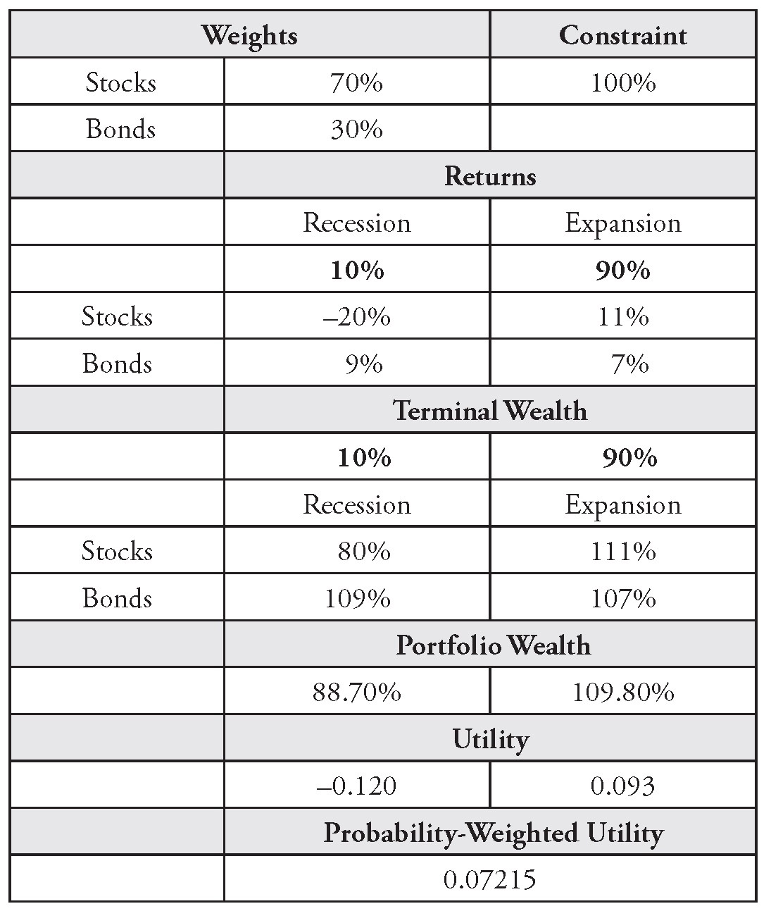
The goal is to maximize probability-weighted utility. To do so, we can try different stocks and bonds weights until we find the mix that produces the highest number.
It may be hard to believe, but this small optimizer that we built in five minutes represents the state of the art in portfolio construction technology. We just need to add more scenarios and assets. This framework is much more powerful than mean-variance optimization, because it accounts for all features of the data, such as fat tails, and it allows for any type of utility functions.
However, there’s a catch. As we add more assets, we can’t manually test all possible portfolio weights to find the asset mix that maximizes utility. Call it the “curse of dimensionality.” With two assets, if we move weights by increments of 1% (which is not very precise but probably good enough), we need to test 101 portfolios. With 3 assets, we need to test 5,151 portfolios. With 5 assets, the number of portfolios to test grows to 4.5 million, and so on. It’s a combinatorial problem. The number grows so fast that at 10 assets, we need to test over 4 trillion portfolios. At 20 assets? 5 million trillion (4,910,371,215,000,000,000,000) portfolios, if we round to the nearest trillion.2 Imagine the scale of the problem if we want to be more precise and vary weights by increments of 0.1% instead of 1%.
In practice, this search-optimization process is computerized, and mathematical shortcuts are taken to converge to a solution faster than if we tried every possible set of weights. Many different tools and software packages are available to approximate a solution. The question is, which tool works best?
To answer this question, shortly after we started our research on full-scale optimization, I set up a “battle of the search algorithms.” I wanted to find out which software would perform best. The answer surprised me and everybody else involved.
First, I set up a sample problem in Excel. I used 20 hedge funds, which I selected because they had highly nonnormal historical return distributions. I applied some constraints to avoid concentrated portfolios.
I used a utility function with two inflection points (“kinks”). These inflection points represent a sharp drop in investor satisfaction. Most investors have a significant aversion to loss, beyond what can be modeled with classical, smooth utility functions. Hence, their utility function drops significantly around zero. (For an example, see Kahneman and Tversky’s, 1979, famous s-shaped value function, derived from prospect theory.)
Suppose that for a specific reason (such as the risk of bankruptcy), you want to avoid a one-year return below –10%, at all costs. In this case, your utility function should drop significantly at –10% as well. Any asset that may contribute to such a scenario (–10% or worse) is heavily penalized or eliminated from your portfolio. Essentially, this drastic kink in the utility function eliminates any solution that may breach the –10% loss barrier, no matter how small the probability of breach or how high the expected return that you need to forgo to eliminate the offending asset. (Remember: There are no free lunches in portfolio construction—only trade-offs.)
I expected this case to be difficult to solve. It involved a relatively large number of assets, with nonnormal return distributions and the added complexity of constraints and kinks in the utility function. I wrote an email to a long list of colleagues to kick off the contest. I included people from our IT department who had access to massive computing power (through a “grid” platform), quant finance whizzes, Harvard PhD economists, etc. My question was simple: “Which set of weights maximizes utility?”
The underlying, more interesting experiment was to find out who would get the highest utility number. All the participants had the same information. They could use any tool they wanted. There would be a clear winner: whoever solved for the highest utility.
My best guess was that a genetic algorithm would win. One colleague had started to work on genetic algorithms. A genetic algorithm uses a wide range of randomly selected starting points, lets them “compete” toward a higher utility number, kills off the least promising areas, and reconcentrates computing power on the most promising searches. (Beyond this simple description, I have no idea how to write a genetic algorithm. But it sounds cool.) Or perhaps someone in IT would win, through the brute force of computing power.
I certainly didn’t expect that I would win. But I did. I generated the highest utility number with the most mundane of all tools: Microsoft Excel’s solver. My takeaway is to never underestimate Microsoft. It turns out that anyone with a basic version of Excel can build a remarkably powerful and flexible full-scale portfolio optimization tool.
While I thought my contest was clever, a few colleagues commented that it wasn’t fair. A fair comparison should cover multiple optimization cases, with different assets, utility functions, and constraints. It should include portfolios with hundreds of individual stocks and bonds. My contest was anecdotal at best. Nonetheless, applied to a utility maximization framework like the one we built in five minutes, the Excel solver works very well. (Of course, multiperiod optimizers, as mentioned earlier in the context of target- date funds glide path design, are much harder to build and represent a whole separate set of challenges.)
Though they impose rigor on the process, utility models don’t always represent investor preferences very well. As we have discussed in the sections on return and risk forecasting, it’s extremely difficult to model risky outcomes. We have two interconnected problems: we apply models that poorly represent investor preferences to estimates that poorly represent investment returns and risks. Yet, to echo the story from my introduction to this book, if we don’t think we can do a reasonable job at both, perhaps we shouldn’t be in the investment business.
A Middle Ground Between Simplicity and Complexity
To approximate utility functions and asset return distributions, it helps to simplify the portfolio construction problem. As Harry Markowitz found, mean-variance optimization achieves this goal remarkably well. Higher moments don’t matter, as Markowitz showed in his debate with Samuelson on the subject. In our research on full-scale optimization, initially we found similar results.
Problems with mean variance start to occur when the utility function includes a sharp drop, a kink that represents significant aversion to loss beyond a threshold. As mentioned, such situations are quite common—most investors define their tolerance to risk as “I can’t lose more than x% in one year.” In these cases, mean-variance optimization allocates too much to assets with low volatility but large exposure to loss (negatively skewed assets that sell volatility). Jan-Hein Cremers, Mark, and I (2005) published these findings in a paper titled “Optimal Hedge Fund Allocations: Do Higher Moments Matter?,” and Tim Adler and Mark (2007) published a more general paper with similar conclusions: “Mean-Variance Versus Full-Scale Optimisation: In and Out of Sample.”
Mean-variance and full-scale portfolio optimization models are bookends on a spectrum from simplest (mean variance) to most complex (full scale). Between these bookends, there are several modified versions of mean- variance optimization that account for fat tails but don’t require us to define a utility function in detail.
For example, in Chapter 11 we discussed risk regimes and how we can model a fat-tailed distribution as a mixture of two probability distributions, each of which may be normal. In a paper that contains the best footnote in the history of the Financial Analysts Journal (more on that shortly), “Optimal Portfolios in Good Times and Bad,” George Chow, Eric Jacquier, Mark Kritzman, and Kenneth Lowry (1999) suggest a blended regime approach. They modify mean-variance optimization to make it more sensitive to exposure to loss. To do so, they use two separate sets of volatilities and correlations (“covariance matrices”): one for the normal regime and one for the turbulent regime. The goal is to find the portfolio weights that maximize
Expected return – [risk aversion 1 × volatility (quiet) + risk aversion 2 × volatility (turbulent)]
where risk aversion 1 represents aversion to volatility in quiet markets and risk aversion 2 represents aversion to risk in times of market stress. As in the original version of mean-variance optimization, volatility is measured as the squared standard deviations of returns.
The authors also multiply the risk aversion terms by the relative probabilities of the quiet and turbulent regimes. Turbulent regimes typically have low probability but significant exposure to loss. Ultimately, regimes can be defined in different ways. In this paper, Chow et al. propose a powerful method that accounts for correlation effects.
They define the regimes based on a measure of multivariate distance, also called the Mahalanobis distance. The Mahalanobis distance is a measure of the distance between a point and the center of a distribution, a multidimensional generalization of the idea of measuring how many standard deviations away the point is from the mean of the distribution. It has a long history of applications in scientific research, and several useful animated tutorials on how to calculate it are available online. It was first used in 1927 to measure similarities in skulls. In 2010, Mark Kritzman and Yuanzhen Li published a paper titled “Skulls, Financial Turbulence, and Risk Management” in the Financial Analysts Journal.
In addition to how far it is from the average, an observation—usually a month in a data sample—is more likely to be a multivariate outlier if it represents an unusual interaction between assets. What does this have to do with skulls? Kritzman and Li explain:
Mahalanobis (1927) used 7–15 characteristics of the human skull to analyze distances and resemblances between various castes and tribes in India. The skull characteristics used by Mahalanobis included head length, head breadth, nasal length, nasal breadth, cephalic index, nasal index, and stature. The characteristics differed by scale and variability. That is, Mahalanobis might have considered a half-inch difference in nasal length between two groups of skulls a significant difference whereas he considered the same difference in head length to be insignificant. . . . He later proposed a more generalized statistical measure of distance, the Mahalanobis distance, which takes into account not only the standard deviations of individual dimensions but also the correlations between dimensions. [Italics added]
It turns out that the approach is useful in an investment context to estimate financial turbulence and define risk regimes. Chow et al. provide an easy visualization of the methodology for two assets. In our State Street PowerPoint presentations, we used a 3D rotating ellipsoid, which helped us explain the concept as applied to three assets (and show off what at the time were impressive animated GIF capabilities). But when we try to visualize an outlier in more than three dimensions, i.e., for four assets or more, it gets much harder. This leads me to a fun footnote. I don’t know how Chow et al. managed to get it passed the referees, but here it is:
If we were to consider three return series, the outlier boundary would be an ellipsoid, a form that looks something like a football. We are unable to visualize an outlier boundary for samples that include more than three return series—at least not without the assistance of a controlled substance.
There are several other modified versions of mean-variance optimization that account for nonnormal (non-Gaussian) higher moments, in particular fat tails.3 For example, we can replace volatility with a measure of tail risk. In Chapter 10 we discussed conditional value at risk (CVaR), a measure of expected loss during market sell-offs. If we use CVaR as our measure of tail risk, we can modify mean variance to solve for the weights that maximize4
– risk aversion × CVaR
CVaR can be replaced with any tail-risk measure of choice, such as probability of a loss greater than –10%, value at risk (VaR), etc.
We can also use tail-risk constraints. For example, suppose we don’t want CVaR to go below –10%. We can define the optimization problem as
Expected return – risk aversion × volatility subject to CVaR <–10%
In this framework, any constraint should work. For example, we can solve for the mean-variance optimal portfolio, subject to a constraint that the portfolio not lose more than 15% under a 2008 historical scenario. This constrained framework also allows for multiple scenario constraints—for example, we can combine 2000 and 2008 scenarios. We can also use forward- looking scenarios.
We can combine volatility and tail risk directly into one objective function. To do so, we can use the same approach as we did for the risk regimes above, but replace the regime-specific aversion parameters with aversions to volatility and tail risk:
Expected return – [risk aversion 1 × volatility (quiet) + risk aversion 2 × tail risk]
Again, tail risk can be measured as CVaR, VaR, probability of loss, 2008 scenario, etc. It can be probability-weighted within the objective function. Essentially, every tail-risk measure we discussed in the risk forecasting section can be used, and beyond. With this approach, we optimize the portfolio in three dimensions: return, volatility, and tail risk. For the same return and volatility, we want the solution with the lowest possible tail risk. Hence, again we penalize assets with low volatility but high tail risk (those pesky “short-volatility” assets, such as hedge funds, credit, and the like).
In Chapter 8 we discussed higher moments. Another methodology is to add these higher moments directly into the objective function, as follows:5
Expected return – risk aversion × volatility + skewness aversion × skewness – kurtosis aversion × kurtosis
Note the positive sign for skewness, as positive skewness is preferable to negative skewness for loss-averse investors. The effect of this modification to mean-variance optimization is generally the same as for the other modified approaches: assets with undesirable downside risk are penalized beyond what would be captured by volatility.
How Should We Address Issues with Concentrated and Unstable Solutions?
Anyone who has used optimizers for portfolio construction knows that they often yield concentrated portfolios. Also, these concentrated solutions can be sensitive to small changes in inputs, which compounds the problem. Counterintuitively, it could be argued that these issues are moot. Before I explain why most people worry too much about them, let me review how they have been addressed in the financial literature.
First, we can apply constraints to the weights. For example, we can limit the hedge fund allocation to 10% of the portfolio. Such constraints can be applied to any of the methodologies described above, from full-scale optimization to all flavors of tail-risk-sensitive mean-variance optimizations.
We can define “group” constraints. Suppose that in addition to stocks and bonds, we allocate to hedge funds, liquid alternatives, and real estate—all asset classes that are part of the “alternatives” category. In this case, we could set up a constraint such that no more than 20% of the portfolio should be allocated to alternatives. (I didn’t pick this example randomly. Alternative assets often have artificially low volatilities and unreasonably high expected returns, which leads to “corner” solutions in which the optimizer allocates the entire portfolio to alternatives. A classic example: If you add private real estate to a stocks and bonds portfolio, and you don’t carefully calibrate your inputs, the optimizer will want to allocate 100% to private real estate.)
There are many other ways to deal with these issues beyond simple weights constraints. Indeed, the literature on how to overcome problems with concentrated portfolios and unstable solutions in portfolio optimization is extensive. A popular approach, pioneered by Richard Michaud, has been to use resampling.6 The idea is to repetitively reoptimize the portfolio on subsamples of our dataset. This process reveals that small changes in data samples can lead to very different solutions. But if we calculate the average of the solutions, we stabilize the outcome.
When short positions are not allowed, this process yields portfolios that are less concentrated. When it resamples, every time the optimizer finds a solution that shorts an asset class, it substitutes the negative weight for a zero allocation. Therefore, the average optimal weight for a given asset is more likely to be positive than if we ran a mean-variance optimization on the full sample. (At least that’s how I understand the process. I believe Michaud employs a few “secret sauce” ingredients as well.)
Though it doesn’t improve our risk and return forecasts per se, this approach can help determine confidence intervals for the optimal weights. We can use it to estimate an optimal “zone” rather than a point estimate. This zone reflects the uncertainty in our estimates.
Another way to impose stability in optimal weights and avoid concentrated portfolios is to use “Bayesian shrinkage” methodologies. Jorion (1986, 1991) proposes an approach that compresses return estimates toward a reference point, such as the average return of the minimum-risk portfolio. This shrinkage process takes into account relative volatilities and correlations across assets to impose consistency in return estimates.
The popular Black-Litterman model uses related concepts, as explained in their 1992 paper, “Global Portfolio Optimization.” The model blends discretionary (what some quants would call “made-up”) views with equilibrium returns (from the CAPM, which we discussed in Chapter 1). This blending process takes into account our level of confidence in our views, as well as volatilities and correlations.
Like the Jorion approach, the Black-Litterman model imposes consistency. If we don’t use views, or if we have very little confidence in them, the solution converges to market capitalization weights. Views that run counter to equilibrium or that would lead to concentrated portfolios are adjusted, or “tamed.” For example, if we expect negatively correlated assets to both experience high positive returns are the same time (which is unlikely since the assets are negatively correlated), the model will likely “shrink” the offending estimate(s) closer to a value consistent with the CAPM.
These shrinkage models are relatively technical, but for quants (or quant-lites like me), the best way to familiarize yourself with them is to recode the example in Black and Litterman’s paper. The authors use a simple three-asset example and provide a step-by-step guide to the process.
These models aren’t that useful for nonquants. They require too many assumptions, and they blur the line between the process to estimate inputs and portfolio construction. If you’re an expert in these models, you can trace back what drives your final estimates: the reference point that you shrink the estimates toward, volatility effects, correlation effects, risk aversion parameters, or other aspects of the models. For everyone else, it is better to cleanly separate return forecasting, risk forecasting, and portfolio construction (incidentally, this is how I’ve organized this book). This separation provides transparency and makes it easier to apply judgment to our estimates.
Another way to avoid concentrated portfolios, with a clearer separation between inputs and portfolio construction than resampling and shrinkage methods, is to add a peer group risk (tracking error) constraint to mean- variance optimization. Even better, as Chow (1995) suggests, we can add tracking error directly to the objective function; i.e., we can maximize
Expected return – risk aversion × volatility – tracking error aversion × tracking error
The tracking error term is like an elastic that pulls portfolio weights toward a benchmark (typically market capitalization weights or the average allocation of a peer group). Tracking error aversion determines the strength of that elastic. In the same way as for the other expanded objective functions we have just reviewed, the aversion parameters enable us to specify the importance of one goal relative to the other. In this case, we can specify whether we care more about absolute risk (volatility) or relative risk (tracking error). Chow shows how this approach yields an efficient surface, as opposed to a traditional efficient frontier. A frontier maps return to risk for optimal portfolios across risk aversion levels. A surface maps return, risk, and tracking error in three dimensions. Chow provides an intuitive visualization:
![]() For the same return and volatility, the optimization finds the portfolio with the lowest tracking error.
For the same return and volatility, the optimization finds the portfolio with the lowest tracking error.
![]() For the same volatility and tracking error, it finds the portfolio with the highest return.
For the same volatility and tracking error, it finds the portfolio with the highest return.
![]() For the same return and tracking error, it finds the portfolio with the lowest volatility.
For the same return and tracking error, it finds the portfolio with the lowest volatility.
To move across the surface, we vary the strengths of the risk aversion and tracking error aversion “elastics.” This idea that the solution set represents an optimal surface, as opposed to a frontier, applies to all optimizations with two risk terms in the objective function, such as the mean-variance–CVaR optimization we discussed above.
Are Optimizers Worthless?
Given the issues with unstable and concentrated portfolios, some academics and practitioners have suggested that optimizers are useless. I disagree. Optimizers are helpful tools if used correctly. If used incorrectly, they can lead to dangerously misallocated portfolios (recall the GIGO critique from the Introduction in this book). In a widely cited paper, DeMiguel, Garlappi, and Uppal (2007) show that equally weighted portfolios outperform mean- variance optimal portfolios across a wide range of assets. I disagree with this conclusion as well.
In “In Defense of Optimization,” Mark Kritzman, Dave Turkington, and I (2010) counter that DeMiguel, Garlappi, and Uppal unfairly penalize mean-variance optimization. These authors feed the mean-variance optimizer the wrong inputs. They use rolling 60-month realized returns as expected returns. But no one would use these assumptions in practice, as they include pathological cases with negative expected equity risk premiums, and broadly speaking, they ignore everything we have discussed in the first section of this book on return forecasting.
In our study, we show that when we use basic expected returns instead of rolling short-term realized returns, mean variance outperforms equally weighted portfolios. We don’t assume any forecasting skill. We model expected returns with long-run averages (estimated out-of-sample) and constant risk premiums. We also use equal returns across assets, which yield the minimum-risk portfolio.
In Chapter 2, I mentioned that risk minimization, without forecasting skill, outperformed the market capitalization–weighted benchmark. In “In Defense of Optimization,” we find similar results across a much broader range of backtests. Again, the takeaway is that without any return forecasts (which is better than with poor return forecasts), optimization performs remarkably well. This result is due to the persistence in volatility and correlations that we discussed in the context of risk forecasting, and perhaps the low-beta effect that we discussed in Chapter 12. Our paper won a 2011 Graham and Dodd Scroll Award for excellence in research.
In the follow-up paper “In Defense of Portfolio Optimization: What If We Can Forecast?,” Allen, Lizieri, and Satchell (2019) expand this research to cases that assume various levels of forecasting skills. Their results reinforce our conclusions. In their words:
We challenge academic consensus that estimation error makes mean-variance portfolio strategies inferior to passive equal-weighted approaches. We demonstrate analytically, via simulation, and empirically that investors endowed with modest forecasting ability benefit substantially from a mean-variance approach. . . . We frame our study realistically using budget constraints, transaction costs and out-of- sample testing for a wide range of investments.
Besides, the concerns with unstable solutions and concentrated portfolio may be overblown. In a paper titled “Are Optimizers Error Maximizers?,”7 Mark Kritzman (2006) demonstrates that the issue with sensitivity to small changes in inputs only occurs when assets are highly correlated, and therefore they can be substituted for each other without a large impact on the portfolio’s return and risk characteristics. Thus, large shifts in weights barely change the risk and return of the optimal solution. And when assets aren’t highly correlated, optimal solutions are more stable.
What About Risk Parity?
With risk parity, we can greatly simplify portfolio construction. I agree that we should put risk at the center of the asset allocation decision and that we should strive for robustness (i.e., find solutions that may be suboptimal under a precise set of return and risk forecasts, but that work reasonably well under a wide range of possibilities). However, asset allocators should not rely naïvely on the approach.
The idea is to equalize asset classes’ contribution to portfolio risk. Think of risk parity portfolios as equal risk portfolios, instead of equal weights. To increase risk contributions from lower-volatility assets, such as bonds, we must lever them. Typically, we assume that all asset classes have the same expected return-to-risk ratio.
Simplifying assumptions are often made for correlations as well. These assumptions are thought to make the process more “robust” because they are somewhat “agnostic” and reduce forecast errors. This idea of robustness has become quite popular with investors, especially after several strategies outperformed the traditional 60% stocks, 40% bonds portfolio during the sell-off of 2008.8 Risk parity products offered by quantitative asset managers have grown to as much as USD 500 billion in AUM, as of 2018.9
In 2016, I reviewed Edward Qian’s book Risk Parity Fundamentals, for the Quantitative Finance Journal.10 Over the last few years, the asset management industry has been divided on the topic of risk parity. Some prominent asset managers seem to religiously believe that it offers better risk-adjusted performance compared with traditional asset allocation approaches, irrespective of where and how it is implemented. Others believe that risk parity is a fad fueled by misleading interpretations of finance theory and dubious backtests.
The debate reached a critical point a few years ago with the publication of an article by Robert Anderson, Stephen Bianchi, and Lisa Goldberg (2012) in the Financial Analysts Journal, titled “Will My Risk Parity Strategy Outperform?” The authors showed that over an 80-year backtest, risk parity underperforms the 60% equities/40% bonds portfolio, after accounting for the historical cost of leverage and turnover.
The response by proponents of risk parity was thoughtful and quite clear. Anderson, Bianchi, and Goldberg’s backtest of risk parity was misleading because it misrepresented how the approach is implemented in practice. Ultimately, our industry seems to have reached the “Let’s agree to disagree” stage of the debate.
Qian’s book is certainly one-sided in favor of risk parity. In almost every chapter, he repeats the mantra that risk parity provides better diversification, and ipso facto better risk-adjusted performance, than traditional balanced portfolios. Toward the end of the book, I started to wonder whether Qian would claim that risk parity can cure cancer. He certainly makes a strong case that to improve portfolio returns, investors should use high return-to-risk ratio, low-beta assets (usually bonds). Such results are consistent with the theory of leverage aversion, which we discussed earlier in the context of the low-beta risk premium.
Most chapters read like a rebuttal to risk parity skeptics. Here are some liberal paraphrases of his questions and answers:
Q: Aren’t bond yields too low?
A: The slope of the curve and what’s priced in matter more than the level of rates.
Q: Does risk parity rely on an unsafe amount of leverage?
A: No. In fact, if we account for the implicit leverage in stocks, risk parity leverage is similar to balanced portfolios.
Q: What if both stocks and bonds become positively correlated, for example, during unexpected rate increases?
A: Historical evidence shows that risk parity portfolios recover well from such episodes. Moreover, commodities provide an additional layer of diversification beyond stocks and bonds. (The events of 2020 may put into question this answer. As liquidity completely dried up, for a while investors sold Treasuries at the same time that equity and commodity markets sold off. These events were a perfect storm for risk parity investors.)
Q: Does risk parity ignore liabilities?
A: The approach can be easily adjusted to account for liabilities and funded ratios.
Unfortunately, across all his backtests and examples, Qian does not address one of the most important issues: the critique by Anderson, Bianchi, and Goldberg regarding the cost of leverage and transaction costs. In the current low-rate environment, the cost of borrowing is extremely low. But for backtests that go back 40+ years, he should adjust for historical LIBOR rates that were as high as 9+%. Qian does not provide his assumptions on this question, and the reader is left wondering whether the consistent drumbeat of “Risk parity beats balanced portfolios” would become muted after leverage and turnover costs adjustments.
Overall, it’s not clear whether risk parity is inherently superior to traditional portfolio construction approaches. Skeptics may take issue with the overemphasis on risk concentration, as opposed to exposure to loss. (A 60% equities/40% bonds portfolio may have 95% exposure to the equity risk factor, but it still has a lower exposure to loss than a 95% equities/5% bonds portfolio.) Though most quantitative investors understand and manage tail risks, it’s not always obvious how risk parity portfolios, most of which are constructed based on volatility, account for nonnormal distributions. Risk parity can be implemented in many ways, which can lead to a wide range of outcomes. Technical details on how covariance matrices are calculated, how and when portfolios are rebalanced, and whether a specific risk is targeted over time matter a great deal.
Nonetheless, for investors who have access to cheap leverage, it’s hard to refute the arguments that we should put risk at the heart of the portfolio construction process and that we should increase exposures to uncorrelated, high return-to-risk ratio assets. Valuation-focused investors who don’t believe that return-to-risk ratios are always equal across all asset classes (or don’t believe that correlations are all the same across asset classes) may arrive at a different portfolio than “risk parity,” but they will still benefit from these insights.
Notes
1. See, for example, Levy and Markowitz (1979), Adler and Kritzman (2007), and Cremers, Kritzman, and Page (2005).
2. See Cremers, Kritzman, and Page (2005).
3. For reviews of some of the literature on this topic, see Harvey, Liechty, Liechty, and Müller (2010), Beardsley, Field, and Xiao (2012), and Rachev, Menn, and Fabozzi (2005). Note that the literature on this topic is extensive (see Greiner’s 2012 comment to the FAJ, for example)—apologies in advance for any reference I may have missed. Here I discuss applications that I and many others have used in practice.
4. See Xiong and Idzorek (2011) as an example.
5. See, for example, Beardsley, Field, and Xiao (2012).
6. Visit https://www.newfrontieradvisors.com/research/articles/optimization-and-portfolio-construction/ for a list of references.
7. This paper also won an award—the 2006 Bernstein-Fabozzi/Jacobs Levy Outstanding Article Award. Perhaps a good topic for those who hope to win an award from a financial practitioner journal is to find a way to defend portfolio optimization.
8. See Mercer (2013).
9. Bridgewater, AQR, Panagora, and many others offer such strategies. See www.forbes.com/sites/simonconstable/2018/02/13/how-trillions-in-risk-parityvolatility-trades-could-sink-the-market/#3e6a7a362e2f.
10. Parts of this section are from this book review, with permission. http://www.tandfonline.com.