
Chapter

Principles of Trading System Design
If not the gods, put the odds on your side.
Introduction
This chapter presents some basic principles of system design. You should try to understand these issues and adapt them to your preferences.
First, assess your trading beliefs—these beliefs are fundamental to your success and should be at the core of your trading system. You may have several strong beliefs, and they can all be used to formulate one or more trading systems. After you have a list of your core beliefs, you can build a trading system around them. Remember, it will not be easy to stick with a system that does not reflect your beliefs.
The six major rules of system design are covered in this chapter in considerable detail. The specific issues to be examined are why your system should have a positive expectation and why you should have a small number of robust rules. The focus in the later sections of this chapter is on money-management aspects such as trading multiple contracts, using risk control, and trading a portfolio of markets. The real difficulties lie in implementing a system, and hence, the chapter ends by explaining why a system should be mechanical.
By the end of this chapter, you should be able to write down your trading beliefs, as well as explain and apply the six basic principles of system design.
What Are Your Trading Beliefs?
You can trade only what you believe; therefore, your beliefs about price action must be at the core of your trading system. This will allow the trading system to reflect your personality, and you are more likely to succeed with such a system over the long run. If you hold many beliefs about price action, you can develop many systems, each reflecting one particular belief. As we will see later, trading multiple systems is one form of diversification that can reduce fluctuations in account equity.
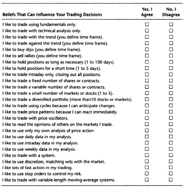
The simplest way to understand your trading beliefs is to list them. Table 2.1 presents a brief checklist to help you get started.
You can expand the items in Table 2.1 to include many other items. For example, you can include beliefs about breakout systems, moving-average methods, or volatility systems. Your trading beliefs are also influenced by what you do. For example, you may be a market marker, with a very short term trading horizon. Or, you may be a proprietary trader for a big bank, trading currencies. You may wish to keep an eye on economic data as one ingredient in your decision process. As a former floor trader, you may like to read the commitment of traders report. Perhaps you were once a buyer of coffee beans for a major manufacturer, and you like to look at crop yield data as you trade coffee. The range of possible beliefs is as varied as individual traders.
You must ensure that your beliefs are consistent. For example, if you like fast action, you probably will not use weekly data, nor hold positions as long as necessary. Nor are you likely to use fundamental data in your analysis. Hence, a need for fast action is more consistent with day trading, and using cycles, patterns, and oscillators with intraday data. Similarly, if you like a trend-following approach, you are more likely to use daily and weekly data, hold positions for more than five days, trade a variable number of contracts, and trade a diversified portfolio. If you hold multiple beliefs, ensure that they are a consistent set and develop models that fit those beliefs. A set of consistent beliefs that can be used to build trading systems is listed below as an example.
- I like to trade with the trend (5 to 50 days).
- I like to trade with a system.
- I like to hold positions as long as necessary (1 to 100 days).
- I like to trade a variable number of shares or contracts.
- I like to use stop orders to control my risk.
Pare down your list to just your top five beliefs. You can review and update this list periodically. When you design trading systems, check that they reflect your five most strongly held beliefs. The next section presents other rules your system must also follow.
Table 2.1 A checklist of your trading beliefs.
Six Cardinal Rules
Once you identify your strongly held trading beliefs, you can switch to the task of building a trading system around those beliefs. The six rules listed below are important considerations in trading system design. You should consider this list a starting point for your own trading system design. You may add other rules based on your experiences and preferences.
- The trading system must have a positive expectation, so that it is “likely to be profitable.”
- The trading system must use a small number of rules, perhaps ten rules or less.
- The trading system must have robust parameter values, usable over many different time periods and markets.
- The trading system must permit trading multiple contracts, if possible.
- The trading system must use risk control, money management, and portfolio design.
- The trading system must be fully mechanical.
There is a seventh, unwritten rule: you must believe in the trading principles governing the trading system. Even as the system reflects your trading beliefs, it must satisfy other rules to be workable. For example, if you want to day-trade, then your short-term, day-trading system must also follow the six rules.
You can easily modify this list. For example, rule 3 suggests that the system must be valid on many markets. You may modify this rule to say the system must work on related markets. For example, you may have a system that trades the currency markets. This system should “work” on all currency markets, such as the Japanese yen, deutsche mark, British pound, and Swiss franc. However, you will not mandate that the system must also work on the grain markets, such as wheat and soybeans. In general, such market-specific systems are more vulnerable to design failures. Hence, you should be careful when you relax the scope of any of the six cardinal rules.
Another way to modify the rules is to look at rule 6, which says that the system must be fully mechanical. For example, you may wish to put in a volatility-based rule that allows you to override the signals. Be as specific as possible in defining the conditions that will permit you to deviate from the system. You can likely test these exceptional situations on past market data, and then directly include the exception rules in your mechanical system design.
In summary, these rules should help you develop sound trading systems. You can add more rules, or modify the existing ones, to build a consistent framework for system design. The following sections discuss these rules in greater detail.
Rule 1: Positive Expectation
A trading system that has a positive expectation is likely to be profitable in the future. The expectation here refers to the dollar profit of the average trade, including all available winning and losing trades. The data may be derived from actual trading or system testing. Some analysts call this your mathematical edge, or simply your “edge” in the markets.
The terms “average trade” and “expectation” represent the same object, so they are freely interchanged in the following discussion. Expectation can be written in many different ways. The following formulations are identical:
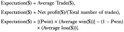
The expectation, measured in dollars, is the profit of the average trade. The net profit, measured in dollars, is the gross profit minus the gross loss over the entire test period. Pwin is the fraction of winning trades, or the probability of winning. The probability of losing trades is given by (1–Pwin). The average win is the average dollar profit of all winning trades. Similarly, the average loss is the average dollar loss of all losing trades.
The expectation must be positive because, on balance, we want the trading system to be profitable. If the expectation is negative, this is a losing system, and money management or risk control cannot overcome its inherent limitations.
Assume that you are using system test results to estimate your average trade. Note that your estimate of the expectation is limited by the available data. If you test your system on another data set, you will get a different estimate of the average trade. If you test your system on different subsets of the same data set, you will find that each subset gives a different result for the average trade. Thus, the expectation of a trading system is not a “hard and fixed” constant. Rather, the expectation changes over time, markets, and data sets. Hence, you should use as long a time period as possible to calculate your expectation.
Since the expectation is not constant, you should stipulate a minimum acceptable value for the average trade. For example, the minimum value should cover your trading costs and provide a “risk premium” to make it attractive. Hence, a value such as $250 for the expectation could be used as a threshold for accepting a system. In general, the larger the value of the average trade, the easier it is to tolerate its fluctuations.
Note that the expectation does not provide any measure of the variability of returns. The standard deviation of the profits of all trades is a good measure of system variability, system volatility, or system risk. Thus, the expectation does not fully quantify the amount of risk (read volatility) that must be absorbed to benefit from its profitability.
The expectation is also related to your risk of ruin. You can use statistical theory to calculate the probability that your starting capital will diminish to some small value. These calculations require assumptions about the probability of winning, the payoff ratio, and the bet size. The payoff ratio can be defined as the ratio of the average winning trades to the average losing trades. As your payoff ratio increases, and your Pwin increases, your risk of ruin decreases. The risk of ruin is also governed by bet size, that is, percentage of capital risked on every trade. The smaller your bet size, the lower the risk of ruin. Detailed calculations of risk of ruin are presented in Chapter 7.
In summary, it is essential that your system have a positive expectation, that is, a profitable average trade. The value of the average trade is not fixed, but changes over time. Hence, you can specify a threshold value, such as $250, before you will accept a trading system. The expectation is also important because it affects your risk of ruin. Avoid trading systems that have a negative expectation when tested over a long time.
The expectation of your system is determined by its trading rules. The next section examines how the number of trading rules affects your system design.
Rule 2: A Small Number of Rules
This book deals with deterministic trading systems using a small number of rules or variables. These trading systems are similar to systems people have developed for tasks such as controlling a chemical process. Their experience suggests that robust, reliable control systems have as few variables as possible.
Consider two well-known trend-following systems. The common dual moving-average system has just two rules. One says to buy the upside crossover, and the other says to sell the downside crossover. Similarly, the popular 20-bar breakout system has at least four rules, two each for entries and exits. You can show with testing software that these systems are profitable over many markets across multiyear time frames.
You can contrast this approach with an expert system-based trading system that may have hundreds of rules. For example, one commercially available system apparently has more than 400 rules. However, it turns out that only one rule is the actual trigger for the trades. The deterministic systems differ from neural-net-based systems that may have an unknown number of rules.
The statistical theory of design of experiments says that even complex processes are controllable using five to seven “main” variables. It is rare for a process to depend on more than ten main variables, and it is quite difficult to reliably control a process that depends on 20 or more variables. It is also rare to find processes that depend on the interactions of four or more variables. Thus, the effect of higher-order interactions is usually insignificant. The goal is to keep the overall number of rules and variables as small as possible.
There are many hazards in designing trading systems with a large number of rules. First, the relative importance of rules decreases as the number of rules increases. Second, the degrees of freedom decrease as the number of rules or variables increases. This means larger amounts of test data are needed to get valid results as the number of rules or variables increases.
A third problem is the danger of curve-fitting the data in the test sample. For example, given a data set, a simple linear regression with just two variables may fit the data adequately. As the number of variables in the regression increases to, say, seven, the line fits the data more closely. Therefore, we can pick up nuances in the data when we curve-fit our trading system, only to pick up patterns that may never repeat in the future. The total degrees of freedom decrease by two for the simple linear regression, but will decrease by seven for the polynomial regression.
These ideas can be illustrated by using regression fits of daily closing data for the December 1995 Standard and Poors 500 (S&P-500) futures contract. The data set covers 95 days from August I, 1995, through December 13, 1995. Two regression lines are fitted to the same data: Figure 2.1 presents a simple linear regression; Figure 2.2 fits higher-order polynomial terms, going out to the fifth power. As higher-order terms are added, the regression line becomes a curve, and we pick up more nuances in the data.
For simplicity, the daily closes are numbered 1 through 95 and denoted by D. All numbers represented by C (such as C1) are constants. Est Close is the closing price estimated from the regression.
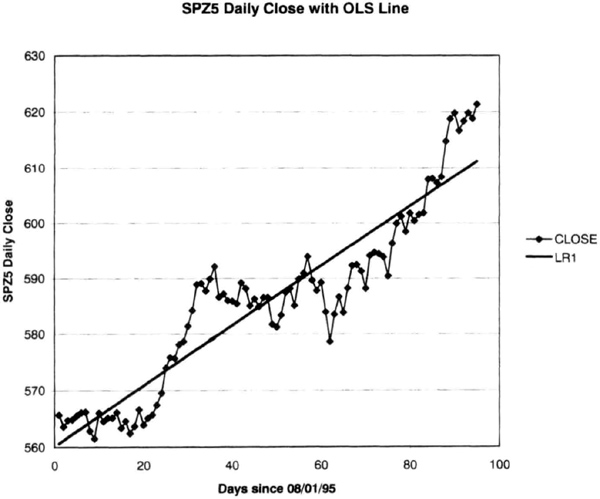
Figure 2.1 S&P-500 closing data with simple linear regression straight line.
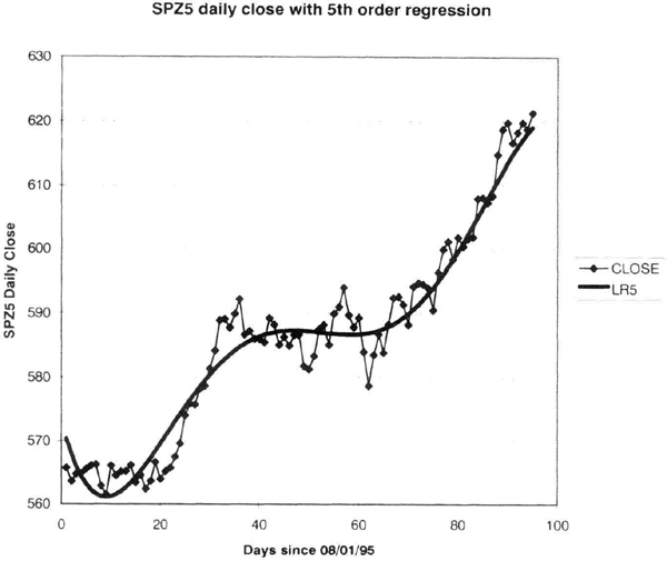
Figure 2.2 S&P-500 closing data with regression using terms raised to the fifth power.

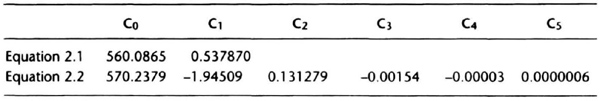
Table 2.2 illustrates several interesting features about curve-fitting a data set. First, observe that the value of the constant C0 is approximately the same for each equation. This implies that the simplest model, the constant C0, captures a substantial amount of information in the data set.
Then, notice that the absolute value of the constants decreases as the order of the term increases. In other words, in absolute value, C0 is greater than C1, which is greater than C2 and on down the line. Therefore, the relative contribution of the higher-order polynomial terms becomes smaller and smaller. However, as you add the higher-order polynomial terms, the line takes on greater curvature and fits the data more closely, as seen in Figures 2.1 and 2.2.
This exercise illustrates many important ideas. First, any model you build for the data should be as simple as possible. In this case, the simple linear regression, with a slope and intercept, captured essentially all the information in the data. Second, adding complexity by adding higher-order terms (read rules) does improve the fit with the data. Thus, we pick up nuances in the data as we build more complex models. The probability that these nuances will repeat exactly is very small. Third, the purpose of our models is to describe how prices have changed over the test period. We used our data to directly calculate the linear regression coefficients. Thus, our model is hostage to the data set. There is no reason why these coefficients should accurately describe any future data. This means that over-fitted trading systems are unlikely to perform as well in the future.
Table 2.2 Comparison of linear regression coefficients.
Another example, a variant of the moving-average crossover system, illustrates why it makes sense to limit the number of rules. In the usual case, the dual moving average system has just two rules. For example, for the long entry the 3-day average should cross over the 65-day average and vice versa.
Now, consider a variant that uses more than two averages. For example, buy on the close if both the 3-day and the 4-day moving averages are above the 65-day average. Since there are two “short” averages, this gives us four rules, two each for long and short trades. Using more and more “short” averages rapidly increases the number of rules. For example, if the 3-, 4-, 5-, 6-, and 7-day moving averages should all be above the 65-day average for the long entry, ten rules would apply.
Consider 10 years of Swiss franc continuous contract data, from January 1, 1985, through December 31, 1994, without any initial stop, but allowing $100 for slippage and commissions. The number of rules is varied from 2 to 128 to explore the effects of increasing the number of rules. As the number of rules increases, the number of trades decreases, as shown in Figure 2.3. This illustrates the fact that as you increase the number of rules, you need more data to perform reliable tests.
Figure 2.4 shows that the profit initially increased as we added more rules. This means that the extra rules first act as filters and eliminate bad trades. As we add even more rules, however, they choke off profits and moreover increase equity curve roughness. Thus, you should be careful to not add dozens of rules.
As stated, this example did not include an initial stop. Hence, as we increase the number of rules, the maximum intraday drawdown should increase because both entries and exits are delayed. You can verify this by using Figure 2.5.
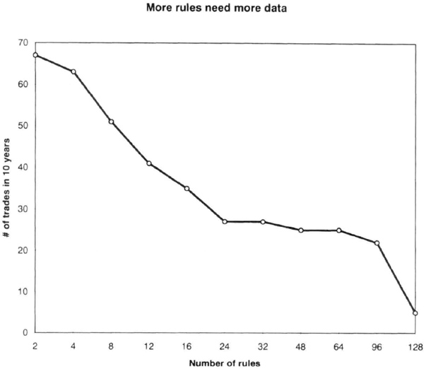
Figure 2.3 Adding rules reduced the number of trades generated over 10 years of Swiss franc data. Note that the horizontal scale is not linear.
Calculations for the U.S. bond market from January 1, 1975, through June 30, 1995, illustrate that the general pattern still holds. Figure 2.6 shows that as the number of rules increases, the profits decrease. The exact patterns will depend on the test data. Data from other markets confirm that increasing rules decreases profits.
Thus, adding rules does not produce endless benefits. Not only do you need more data, but the rising complexity may lead to worsening system performance. A complex system with many rules merely captures nuances within the test data, but these patterns may never repeat. Hence, relatively simple systems are likely to perform better in the future.
Rule 3: Robust Trading Rules
Robust trading rules can handle a variety of market conditions. The performance of such systems is not sensitive to small changes in parameter values.
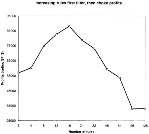
Figure 2.4 Adding rules increased profits moderately on 10-years of Swiss franc continuous contracts from January 1, 1985, through December 31, 1994. Note that the horizontal scale is not linear.
Usually, these rules are profitable over multiperiod testing, as well as over many different markets. Robust rules avoid curve-fitting, and are likely to work in the future.
An example of a system with delayed long entries illustrates the use of nonrobust parameters. The entry rule is as follows: if the crossover between 3-and 12-day simple moving averages (SMAs) occurred x days ago, and the low is greater than the parabolic, then buy tomorrow at the today’s high + 1 point on a buy stop. A $1,500 initial stop was used and $100 was charged for slippage and commissions (Figure 2.7).
The results above are for an IMM (International Monetary Market) Japanese yen futures continuous contract, from August 2, 1976 through June 30, 1995. The dollar profits are sensitive to the number of days of delay, and can vary widely due to small changes in parameter values. It also does not seem reasonable to wait 12 days after a crossover for such short-term moving averages. Hence, the flattening out of the curve after a 9-day delay is of little practical relevance. The delay parameter is not robust because a small change in the value of this parameter can make system performance vary widely with markets and time frames.
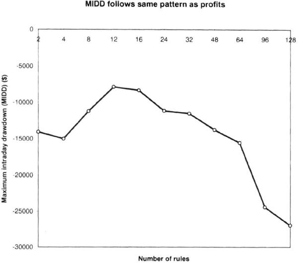
Figure 2.5 Adding more rules delayed entries and exits, increasing maximum intraday drawdown. Note that the horizontal scale is not linear.
Next consider the effect of nonrobust, curve-fitted rules, illustrated by the August 1995 N.Y. light crude oil futures contract (Figure 2.8). The market was in a narrow trading range during February and March, and then broke out above the $18.00 per barrel price level. The market moved up quickly, reaching the $20 level by May. A volatile consolidation period ensued through June, before prices broke down toward the $17 per barrel level by July.
The following trading rules were derived simply by visual inspection of the price chart in an attempt to develop a curve-fitted system that picked up specific patterns in this contract.
Rule 1: Buy tomorrow at highest 50-day high + 5 points on a buy stop (breakout rule).
Rule 2: Sell tomorrow at low −2 × (h-1) − 5 points on a sell stop (down-side range-expansion rule).
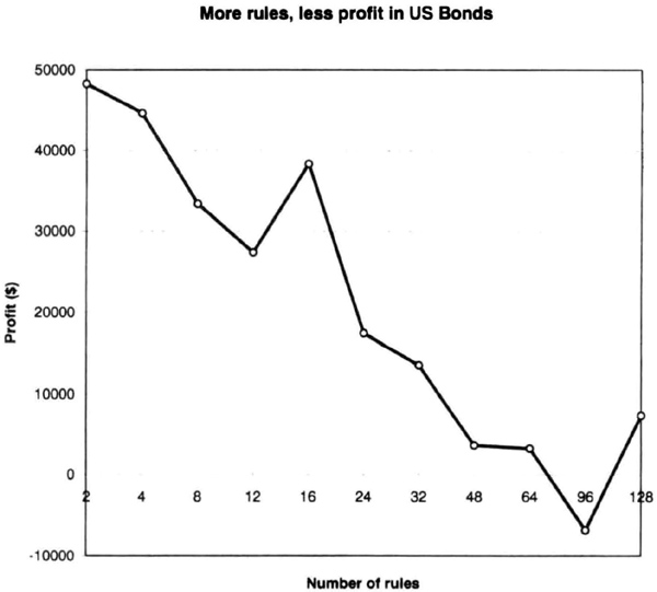
Figure 2.6 Increasing the number of rules decreased profits in the U.S. bond market from January 1, 1975 through June 30, 1995. Note that the horizontal scale is not linear.
Rule 3: If this is the twenty-first day in the trade, then exit short trades on the close (time-based exit rule).
Rule 4: If Rule 3 is triggered, then buy two contracts on the close (countertrend entry rule).
Rule 5: If short, then sell tomorrow at the highest high of last 3 days +1 point limit (sell rallies rule).
The first rule is a typical breakout system entry rule, albeit for a breakout over prior 50-bar trading range. The second rule is a volatility-inspired sell rule. The idea was to sell at a point five ticks below twice the previous day’s trading range subtracted from the previous low. This will typically be triggered after a narrow-range day, if the daily range expands on the downside due to selling near an intermediate high. The third rule is a time-dependent exit rule, optimized by visual inspection over the August contract. The idea behind time-based exits is that one expects a reaction opposite the intermediate trend after x days of trending prices. Rule 4 merely reinforces rule 3 by not only exiting the short position but putting on a two-contract long position at the close. Rule 5 is a conscious attempt to sell rallies during downtrends. In this case, limit orders were used to sell, to avoid slippage. These rules assumed that as many as nine contracts could be traded at one time, using a $1,000 initial money-management stop.
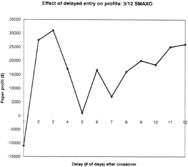
Figure 2.7 The effect on profits of changing the number of days of delay in accepting a crossover signal of a 3-day SMA by 12-day SMA system is highly dependent on the delay.
The results of the testing are summarized in Table 2.3. The first clue that this may be a curve-fitted system is the number of profitable trades. As many as 87 percent of all trades (20 out of 23) were profitable. A second clue was in the 14 consecutive profitable trades. A third clue was in a suspiciously large profit factor (= gross profit/gross loss) of 13.49. These results are what you might see in curve-fitted systems tested over a relatively short time period. The computer-generated buy and sell signals are shown in Figure 2.8.
This curve-fitted system was tested by using a continuous contract of crude oil futures data from January 3, 1989, through June 30, 1995. Not surprisingly, this system would have lost $107,870 on paper, as shown in Table 2.4. Note how only 32 percent of the trades would have been profitable. There would have been as many as 48 consecutive losing trades, requiring quite an act of faith to continue trading this system. Also, the profit factor was a less impressive 0.61, a sharp drop from the 13.49 value in Table 2.3. These calculations show that curve-fitted systems may not work over long periods of time.
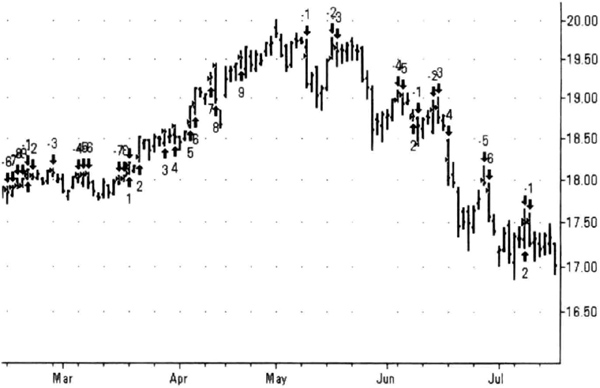
Figure 2.8 The August 1995 crude oil contract with curve-fitted system.
Table 2.3 Results of testing August 1995 crude oil curve-fitted system.
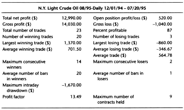
Table 2.4 Results of testing crude oil curve-fitted system over a long time period.

Interestingly, this system has its merits. When tested over 12 other markets to check if these rules were robust enough to use across many markets (Table 2.5), the results were better than expected; on some markets the system tested very well. This result was surprising because (1) this particular combination of rules had never been tested on these markets and were derived by inspection of just one chart; and (2) the long entries and short entries are asymmetric. A symmetrical trading system uses identical rules for entries and exits, except that the signs of the required changes are reversed. For example, a moving average system would require an upside crossover or a downside crossunder for signals.
Table 2.5 A check for robustness: crude oil curve-fitted system over 12 markets (test period: 1/3/89-6/30/95, using continuous contracts, S100 slippage, and commission charge).
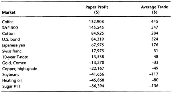
A closer look at the rules shows that they do follow some sound principles. For example, during an uptrend, each successive 50-bar breakout adds a contract until nine contracts are acquired. Thus, market exposure is increased during strong uptrends. The sell rule tends to lock in profits close to intermediate highs. As we sell rallies in downtrends, we are increasing exposure in the direction of the intermediate term trend. Also, a relatively tight $1,000 initial money management stop was used. Thus, even though these rules were derived by inspection, they followed sound principles of following the trend, adding to with-the-trend positions, letting profits run, and cutting losses quickly.
In summary, it is easy to develop a curve-fitted system over a short test sample. If these rules are not robust, they will not be profitable over many different market conditions. Hence, they will not be profitable over long time periods and many markets. Such rules are unlikely to be consistently profitable in the future. Hence, you should try to develop robust trading systems.
Rule 4: Trading Multiple Contracts
Multiple contracts allow you to make larger profits when you are right. However, the drawdowns are larger if you are wrong. You are betting that with good risk control, the overall profits will be greater than the drawdowns. An essential requirement is that your account equity must be sufficiently large to permit trading multiple contracts. Your risk control guidelines must permit multiple contracts to benefit from this approach. If your account permits you to trade just one contract at a time, then this approach must be deferred until your equity has increased.
Multiple contracts also allow you to add a nonlinear element to your system design. This means the results of trading, say, five contracts using this nonlinear logic are better than trading five contracts using the usual linear logic. The linear logic trades one contract per signal. The nonlinear logic uses a price-based criterion such as volatility. The volatility rule buys more contracts when volatility is low. Markets often have low volatility after they have consolidated for many weeks. If a strong trend develops as the market emerges from the consolidation, then the nonlinear effect is to boost profits significantly.
A simple example illustrates these ideas. Assume that your account is so large that trading up to 15 contracts in the 10-year T-note market is well within your risk control guidelines. For example, with a 1 percent risk per position and a $1,000 initial money management stop, you would need $1,500,000 in equity to trade 15 T-note contracts. This assumes that the 15-lot margin is also within your money-management guidelines.
Consider a simple moving average crossover system using 5-day and 50-day simple moving averages. The trade day is one day after the crossover day. You will buy or sell on the next day’s open if you get a 5/50 crossover tonight after the close. Use a $1,000 initial stop on each contract and allow $100 for slippage and commissions.
Let us compare system performance with one contract versus variable contracts, rising to a maximum of 15 contracts. The test period is from January 3, 1989, through June 30, 1995, using a continuous contract. Table 2.6 compares four variations of the 5/50 crossover system. The column labeled “fixed 1 contract” shows the results over the test period for always trading one contract per trade. The next column, “fixed 15 contracts” shows the calculated results for always trading 15 contracts per trade. The column, “variable #1” trades a maximum of 15 contracts with the contracts added at the open on successive days. The “variable #2” trades a maximum of 15 contracts with all the contracts bought on the same day. The volatility in dollars here is four times the average 20-day true range. The volatility divided into $15,000 gives the number of contracts. Thus, variable #2 uses a volatility-based criterion for calculating the number of contracts, always trading 15 or less.
Table 2.6 Performance comparison using variable number of contracts.
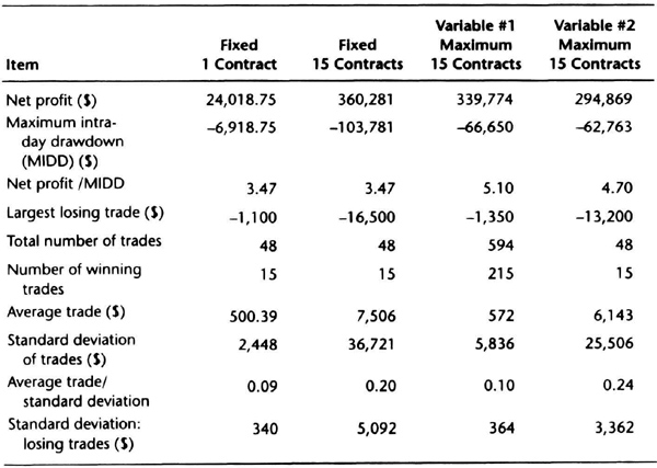
Let us compare the net profit produced by the four strategies. It should come as no surprise that the absolute amount of profit increases as we trade more contracts. However, as the next row of Table 2.6 shows, the maximum intraday drawdown also increases as we trade more contracts. The ratio of net profits to maximum intraday drawdown shows whether we gain anything by trading multiple contracts. This ratio is 3.47 for fixed contract trading strategy. The ratio increases to 4.7 or 5.1 for the variable contracts strategies. This is a 39 to 47 percent improvement, a strong reason to consider multiple contracts. Hence, profits can increase without proportionately increasing drawdowns.
Observe from Table 2.6 that the largest losing trade for variable #1 is considerably less than simply trading a fixed number of 15 contracts. Similarly, the largest losing trade in variable #2 is less than always trading 15 contracts. This too confirms the benefits of going to the multiple-contract strategy.
The total number of trades remains the same for the fixed-1, fixed-15 and variable #2 strategies, since all the contracts are bought on the same day. The number of trades increases for variable #1 since not all the contracts are bought on the same day.
The average trade for each strategy is relatively high, suggesting that this simple model seems to catch significant trends. The average trade is higher when all the contracts are bought at the same time. This is merely an artifact of system design. As pointed out before, the average trade does not provide a measure of variability in system results.
The standard deviation per trade is naturally smaller when we trade one contract at a time rather than all at once. The standard deviation in trade returns increases as the number of contracts increases. As Table 2.6 shows, there is a higher volatility in trade returns ($36,721) for fixed 15-contract trading than either of the variable contract strategies. This means volatility can be reduced by trading a variable number of multiple contracts, rather than a fixed number of multiple contracts. This is another desirable design goal.
Dividing the average trade profit by the standard deviation in trade profitability yields a composite picture of model performance. The higher this number, the more desirable the system. For the fixed 1-contract strategy, this reward to risk ratio is only 0.09, and it increases to 0.24 for the variable #2 strategy. Remember, however, that the volatility in trading profits increases significantly with multiple contracts.
The last line of Table 2.6, the downside volatility, explains that the increased volatility occurs due to rising profits of winning trades. Note that the fixed 15-contract downside volatility is the highest, followed by the variable #2 and variable #1 strategies. There is not a large difference in downside volatility between the fixed 1-contract strategy and variable #1 strategy, which buys one contract at a time but on multiple days. Note also that the standard deviation of all trades (including winning trades) is much greater than the downside volatility. Thus, rather than all volatility being undesirable, note that adding multiple contracts increases upside volatility more than downside volatility. Increasing upside volatility is easier to cope with than sharply rising downside volatility.
In summary, if your account equity and mental makeup permit, consider the benefits of a multiple contract strategy.
Rule 5: Risk Control, Money Management, and Portfolio Design
All traders have accounts of finite size as well as written or unwritten guidelines for expected performance over the immediate future. These performance guidelines have a great influence over the existence and longevity of an account. For example, consider a trading system that produces a 30 percent loss over five months. The same trading system then goes on to perform extremely well. One person may close the account after the 30 percent drawdown. Another may go on to reap excellent returns. Your money management rules could cause you to close out an account too soon, or keep it open too long. Thus, money management guidelines are crucial to trading success.
Given performance expectations and finite size of the trading account, it is essential to maintain good risk control, sensible money management, and good portfolio design. Risk control is the process of managing open trades with predefined exit orders. Money management rules determine how many contracts to trade in a given market and the amount of money to risk on particular positions. Portfolio-level issues must be considered to obtain a smoother equity curve.
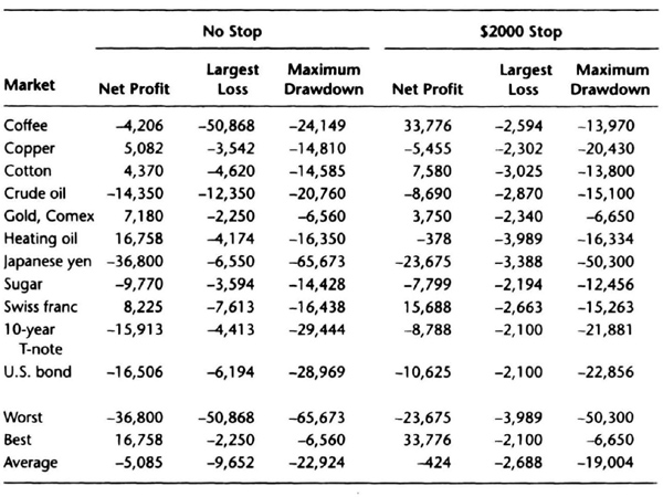
Table 2.7 illustrates the effects of not using an initial money management stop versus adding an initial money management stop of $2,000. The trading system, a “canned” system using four consecutive up or down closes to initiate a trade, comes with the Omega Research’s System Writer Plus™.
As expected, the largest losing trade can be horrifying, and most real-world accounts would probably close before swallowing such huge losses. Of course, recent headlines of billion-dollar plus losses in sophisticated trading firms illustrate that trading without adequate risk control is not uncommon.
Adding a money management stop constrains the worst initial loss to predictable levels. Even with slippage, the largest loss is usually lower than trading without any stop at all. Thus, your profitability is likely to improve with improved risk control. Observe that average net profits improved from a loss of –$5,085 with no stop to a loss of –$424 using risk control. The maximum drawdown also improved with the added risk control. The lesson from this comparison is clear. There is much to gain if you use proper risk control.
You can reduce swings in equity and improve account longevity if you combine risk control with sound money management ideas. Your money management guidelines will specify how much of your equity to risk on any trade. These guidelines convert the initial stop into a specific percentage of your equity. One common rule of thumb is to risk or “bet” just 2 percent of your account equity per trade.
Table 2.7 Effect of adding an initial money management stop, May 1989–June
The 2-percent rule converts into a $1,000 initial stop for a $50,000 account. This $1,000 initial stop is often called a “hard dollar stop,” applied to the entire position. A position could have one or more contracts. Thus, if you had two contracts, you would protect the position with a stop loss order placed $500 away from the entry price. Chapter 7 discusses the bet size issue in detail.
Overtrading an account is a common problem cited by analysts for many account closures. For example, if you consistently bet more than 2 percent per trade, you are overtrading an account. If you do not use any initial money management stop, then the risk could be much greater than 2 percent of equity. In the worst case, you risk your entire account equity. Some extra risk, say up to 5 percent of equity, may be justified if the market presents an extraordinary market opportunity (see Chapter 4). However, consistently exceeding the 2 percent limit can cause large and unforeseen swings in account equity.
As another rule of thumb, you are overtrading an account if the monthly equity swings are often greater than 20 percent. Again, there may be an occasional exception due to extraordinary market conditions.
You must also consider the benefits and problems of diversification, that is, trading many different markets in a single account. The main advantage of trading many markets is that it increases the odds of participating in major moves. The main problem is that many of the markets respond to the same or similar fundamental forces, so their price moves are highly correlated in time. Therefore, trading many correlated markets is similar to trading multiple contracts in one market.
For example, the Swiss franc (SF) and deutsche mark (DM) often move together, and trading both these markets is equivalent to trading multiple contracts in either the franc or the mark. Let us look specifically at SF and DM continuous contracts from May 26, 1989, through June 30, 1995, with a dual moving average system using a $1,500 stop and $100 for slippage and commissions. The two moving averages were 7 and 65 days. As Figure 2.9 shows, the equity curves have a correlation of 83 percent. For example, you would have made $60,619 trading one contract each of SF and DM, but your profits would have been $63,850 trading two contracts of DM and $57,388 trading two contracts of SF.
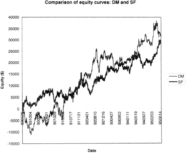
Figure 2.9 Swiss franc and deutsche mark equity curves are highly correlated at 83 percent.
Note one important difference between the two cases. Since the two markets may have negative correlation from time to time, the drawdown for both SF and DM together may be in between trading two contracts of just DM or SF. For example, the drawdown for SF and DM in this case was –$10,186 versus –$22,375 for two DM contracts and –$9,950 for two SF contracts. Hence, the benefits of trading correlated markets are relatively small. Thus, it may be better to trade uncorrelated or weakly correlated markets in the same portfolio.
The benefits of adding usually unrelated markets to a portfolio can be illustrated by an example of trading the Swiss franc (SF), cotton (CT) and 10-year Treasury note (TY) in a single account, using the same dual moving average system as above. The paper profits from trading three SF contracts add up to $86,801 versus $85,683 for SF plus TY and CT. The equity curve for the two combinations is shown in Figure 2.10. The smoothness of the two curves can be compared by using linear regression analysis to calculate the standard error (SE) of the daily equity curve. The SE for trading three SF contracts in $6238, and the SE for SF and TY plus CT is just $4,902, a reduction of 21 percent. Thus, adding TY and CT to a portfolio of SF produced a smoother equity curve with essentially the same nominal profits.
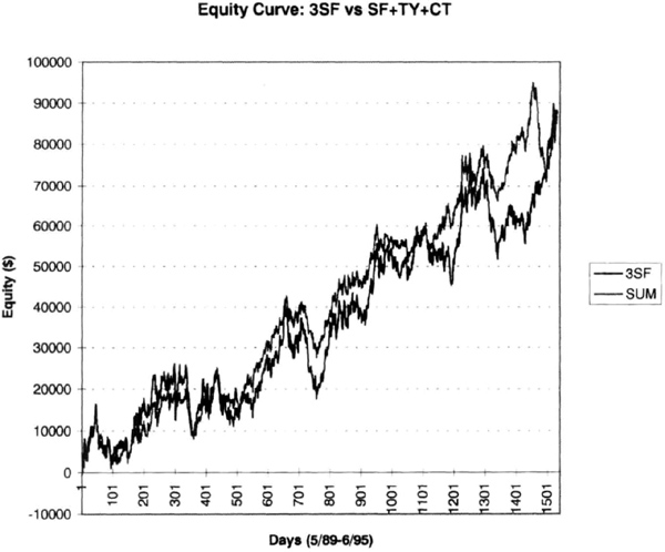
Figure 2.10 Adding 10-year T-note (TY) and cotton to the portfolio trading just Swiss francs provides a smoother equity curve versus trading three SF contracts.
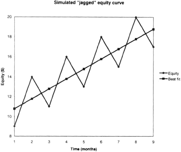
Figure 2.11 This contrived jagged equity curve has a standard error of 2.25. The perfectly smooth equity curve has an SE of zero. The standard deviation of monthly returns is 33 percent.
The relevance of the standard error is illustrated in Figure 2.11, which shows a contrived equity curve. The SE for that curve was 2.25, since it was quite “jagged.” A perfectly smooth equity would have an SE reading of zero.
Diversification can be more than just adding markets. You can also trade multiple trading systems and multiple time frames within a single account. You should try to use uncorrelated or weakly correlated systems. In summary, risk control, money management, and portfolio design are important issues in designing trading systems.
Rule 6: Fully Mechanical System
The simplest answer to why a system must be mechanical is that you cannot test a discretionary system over historical data. It is impossible to forecast what market conditions you will face in future and how you will react to those conditions. Therefore, in this book, we will restrict ourselves to fully mechanical systems.
If you can define how you make discretionary decisions, then these rules could be formalized and tested. The process of formalization could itself provide many interesting ideas for further testing. Hence you are encouraged to move toward mechanical systems.
You are more likely to make consistent trading decisions if you use mechanical systems. The manner in which a mechanical system will process price data is predictable, and hence assures that you will make consistent trading decisions. However, there is no assurance that these logically consistent decisions will also be consistently profitable. Nor is there any assurance that these trading decisions will be implemented without modification by the trader.
Summary
This chapter developed a checklist for narrowing your trading beliefs. You should narrow your beliefs down to five or less to build effective trading systems around them.
This chapter also reviewed six major rules of the system design. A trading system with a positive expectation is likely to be profitable in the future. The number of rules in a system should be limited because increasing complexity often hurts performance. Relatively simple systems are likely to fare better in the future. The rules should be robust, so they will be profitable over long periods and over many markets. You should trade multiple contracts if possible because they allow you to make more profits when you are right. Risk control, money management, and portfolio design give you a smoother equity curve and are the keys to profitability. Lastly, a system should be mechanical to provide consistent, objective decision making. You should follow the six major rules to build superior systems that are consistent with your trading beliefs.