Chapter

Developing New Trading Systems

Don’t count your chickens until they are incubated.

Introduction

A trading system is only as good as your market intuition. You can formulate and test virtually any trading system you can imagine with today’s software. The previous chapters studied the basic principles of system design. This chapter develops and tests several original trading systems to illustrate the application of those principles:

1. A simple trend-following system—the 65sma-3cc system.
2. A pattern-based system for long trades only—the CB-PB system.
3. A trend-seeking, strength-of-trend system—the ADX burst system.
4. An automatic mode-switching system—the trend-antitrend system.
5. Intermarket systems for correlated markets—the gold bond systems.
6. A system for picking bottoms—a bottom-fishing pattern.
7. A system for increasing bet size—the extraordinary opportunity model.

In this chapter, each case illustrates a different design philosophy. The 65sma-3cc system is examined in the greatest detail; the same principles can be applied to all other systems. Long-term test results with continuous contracts are shown for every system.

This is not a recommendation that you trade these systems. These systems have all the limitations of hypothetical test results. They are discussed here only as examples of the art of developing systems that suit your trading style.

The Assumptions behind Trend-Following Systems

The basic assumptions behind a simple trend-following system are as follows:

1. Markets trend smoothly up and down, and trends last a long time.
2. A close beyond a moving average signals a trend change.
3. Markets do not have large countertrend price swings.
4. Prices do not move too far away from an intermediate moving average.
5. Whipsaws are relatively few and do not cause large losses.
6. Significant price moves last many weeks or months.
7. Markets are predominantly in a trending mode.

The reality of a trend-following system is that:

1. Markets are often in ranging mode with choppy swing moves, so losses in trading ranges are significant.
2. There are large swings in trade equity, since the model “gives back” a large proportion of profits before signaling an opposite trend.
3. These systems need a relatively “loose” stop in order to avoid missing about 5 percent of trades that account for major profitable moves.
4. These systems often enter the market on strength or weakness, so that they can be stopped out during short but vicious countertrend moves.

The advantages of simple trend-following systems are:

1. They provide guaranteed entry in the directions of the major trend.
2. They are profitable over multiple markets and multiple time frames, as long as time frames are 6 months to 5 years in horizon.
3. These systems are usually robust.
4. These systems have well-defined risk-control parameters.

The 65sma-3cc Trend-Following System

This section discusses how to formulate and test a simple, nonoptimized, trend-following system that makes as few assumptions as possible about price action. It arbitrarily uses a 65-day simple moving average of the daily close to measure the trend. Sixty-five days is simply the daily equivalent of a 13-week SMA (13 × 5 = 65), representing one-quarter of the year. This is an intermediate length moving average that will consistently follow a market’s major trend.

As shown in Figure 4.1, when the market is trending up, prices are above the 65-day SMA, and vice versa. In sideways markets, this SMA flattens out and prices fluctuate on either side. Clearly, the trading system picks up and sticks with the prevailing trend (see Figure 4.2).

There are many ways to make the decision that the trend has turned up. The usual way is to use a shorter moving average of, say, 10 days, and decide that the trend has changed when the shorter average crosses over or under the longer moving average. If you decide to use a short moving average, its “length” will be crucial to your results. Another weakness is that often prices will move faster than the shorter moving average, so that the entries can seem rather slow.

Hence, the 65sma-3cc system will require three consecutive closes (3cc) above or below the 65-day SMA (65sma) to determine that the trend has changed. For example, the trend will be said to have turned up after three consecutive closes above the 65-day SMA. Similarly, the trend will have turned down after three consecutive closes below the 65sma. Once again, the requirement of three consecutive closes is arbitrary. It could be ten consecutive closes or any other number. Clearly, the results will vary with the number of confirming closes.

Figure 4.1 September 1995 Japanese yen contract showing the 65-day SMA and the signals generated by the system.

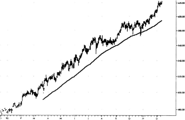
Figure 4.2 The 65sma-3cc system stayed long throughout this major uptrend in the S&P-500 index in 1995.

If you are afraid of false signals (see Figure 4.3), then the number of closes you use will act like a filter in reducing the number of trades. In a fast-moving market, requiring a large number of consecutive closes will give delayed entries (see Figure 4.4). Conversely, if a market is moving sluggishly, a small number of consecutive closes will give false signals. Thus, there is a trade-off here that determines how quickly you recognize a change in trend.

Once you recognize a change in trend, you still have to decide how to enter the trade. You should enter the trade on the next day’s open, to guarantee that you can execute the signal and get a fill. For example, if the three consecutive closes criterion is satisfied as of this evening’s close, you should buy at the market on the open of the next trading day. You will get a fill somewhere in the opening range the next day. It is likely that you will be filled near the top of the opening range for buy orders, and near the bottom of the opening range for sell orders. This slippage should be ignored, and just lumped into your $100 allowance for slippage and commissions. The main effect of this entry mechanism is that you are not filtering out any entry signals, and ensuring that you will put on this position the first time the entry conditions are satisfied.

Figure 4.3 The choppy sideways action in December 1995 British Pound generated a string of whipsaw losses for the 65sma-3cc system.

Figure 4.4 These swing moves in December 1995 crude oil produced many trades but small profits because the 65sma-3cc system does not have a specific exit strategy.

There are a number of choices on how to actually enter the trade. For example, you could enter the trade on the close of the third consecutive close above or below the 65sma. A second choice would be to enter the next day on a stop order beyond the previous, or a nearby, high or low. In effect, you would also filter out some entry signals, because you would not get a fill on every signal. This may be useful in situations where prices briefly spike beyond the 65sma during prolonged trends.

A third entry choice would be to delay entry for x days after the signal, and then enter beyond a nearby n-day high or low. This is another way to filter down the entry signals in order to find more profitable ones. Note that if you use a limit order for your entries, occasionally you may not be filled at all, missing the entry by just a few ticks. Hence, you should enter on the next day’s open to assure an entry into the new trend.

Before we proceed, let us put this entry signal through a critical test to check if the 65sma-3cc entries are better than random. Following the approach of Le Beau and Lucas (see bibliography for details), let us test the entry signal with exit on the close of the n-th day, without any stops, and no deductions for slippage and commissions. For simplicity, only the effect of long entries are shown. The proportion of trades that are winners should consistently be more than 55 percent. The test includes the long entry over 21 markets, stretching from January 1, 1975, through July 10, 1995, using a continuous contract. Because not all markets were trading back in 1975, all available data are used.

Table 4.1 shows that, on average, 55 percent of the long entries were profitable, suggesting that the 65sma-3cc model probably does better than random. The result for short trades is similar, and you can be reasonably confident that this model provides robust entry signals. Your task is now to combine this model with risk control and exit methods that match your trading mentality.

To summarize this nonoptirnized system, the actual trade entry is at the market on the open of the next trading day after the close of the day the signal is received. You will notice that there are no specific exit signals at this point, which means that the short entry signal is also the long exit signal, and vice versa. In practice this means that if you are long one contract, you will sell two contracts to go net short one contract, and vice versa.

Note that for the tests below we will add a condition to prevent back-to-back entries of the same type. This will allow an apples-to-apples comparison when studying the effect of adding stops or exits. You do not need this condition for actual trading.

To summarize what is not defined at this point: There are no specific risk-control rules in terms of an initial money management stop, nor any money-management rules to determine the number of contracts to trade. We will just trade one contract for simplicity without any risk-control stop. This is not a recommendation to trade without a risk control stop; the calculations are done without any stops here to illustrate a point. Later, we will examine how to add risk control and study the effect of money management.

Table 4.1 Testing 65sma-3cc long entry for randomness over 21 markets using all available data between 1/1/75 and 7/10/95. Exit on the close of the n-th day.

The 65sma-3cc system should make all its profits during strong trends. It should lose money in sideways or nontrending markets. And it should have between 20 and 50 percent profitable trades. We tested this model over 23 markets using 20 years of continuous contract data. If a contract was not traded for 20 years, then we used all available data from the starting date. The usual allowance of $100 per trade for slippage and commissions was made. Thus, this is a rigorous test for a nonoptimized system over a long test period, and across a large number of markets. The results are summarized in Table 4.2.

The results for this simple, nonoptimized trend-following system are encouraging. You could have made a paper profit of $1,386,747 by trading just one contract for each market, and been profitable on 19 of 23 widely diverging markets. The test sample generated 2,400 trades, so this is a highly significant test. Approximately 34 percent of all trades were profitable, a number typical of trend-following systems.

Table 4.2 Test results for 65sma-3cc trend-following system.

The ratio of average winning to average losing trades was excellent, at 3.3 averaged over the 2,400 trades. This number is useful for calculating the risk of ruin; a number above 2.0 is desirable, and anything over 3 is welcome news. The average trade made a profit of $558, an attractive amount, considering transaction and slippage costs. It is customary to seek a number over $250 for the average trade. The average profit per market was $60,293, approximately 2.74 times the average maximum intraday drawdown, of –$22,014. This is a healthy recovery factor, or coverage of the worst losing streak of the system.

In summary, a simple trend-following approach worked on many markets over a long time period with few assumptions and no optimization.

The results also point out some weaknesses of this system. The average profit per market is 90 percent of the standard deviation of the average profit. This means that profitability varied widely from market to market. The maximum intraday drawdown was 108 percent of its standard deviation, implying that the drawdowns also varied considerably among markets. The standard deviation of the average trade also implies that results can vary substantially over time or across markets. A further weakness is the relatively small number of profitable trades. Thus, we can summarize the principal weakness as a large variability in the results over time and across markets.

Combining the strengths and weaknesses, you would say that this is a sound trend-following system with good chance of being profitable over many markets over a long time period. But because of the large variability in results, you would have to trade this system relatively conservatively. You should allow a large equity cushion to absorb drawdowns.

A look under the hood of this trading system, so to speak, and a closer examination of the results of the analysis reveal further details of 65sma-3cc trades. A histogram of all 2,400 trades shows the distribution of trade profits and losses (see Figures 4.5 and 4.6). There are more large winners than large losers, and many small losers. Remember that these results were calculated without using an initial money management stop. Most of the trades are bunched between –$3,000 and $2,000, with the highest frequency near zero. There are few losing trades worse than –$5,000, balanced by even more trades with profits greater than $5,000. An initial money management stop will clean up the negative part of this histogram.

Thus, it should be obvious that most of the profits come from a relatively small number of trades. In Figure 4.6, 12.5 percent of the trades are seen to have closed-out profit greater than $3,000. Be aware that if you get out too soon, you are likely to miss one of 100 or so (4 percent) of the mega-trades that make trend-following worth the aggravation.

Many measurements follow what is called a standard normal distribution. For example, if you measured the diameter of ball bearings, the measurements will follow a normal distribution. The normal distribution is a bell-shaped probability distribution of the relative frequency of events. The standard normal is a special case of the normal distribution with a mean of zero and standard deviation equal to one. To compare the distribution of the 65sma-3cc trades to the standard normal distribution, we first have to “normalize” the bin sizes. The comparison is shown in Figure 4.7.

Figure 4.5 Histogram of all 2,400 trades for the 65sma-3cc trading system.

The 65sma-3cc curve is more sharply peaked than the standard normal curve. To generate a normal distribution that would fit our data, I used a Microsoft Excel® 5.0 spreadsheet and employed an iterative process of manually tweaking the values. The fitted normal curve, with a mean of –0.16 and standard deviation of 0.18 is shown in Figure 4.8. The fitted normal distribution shows that the actual 65sma-3cc distribution has “fat” tails. This simply means that there is a larger probability for the “big” trades than would be expected from the normal distribution. This chart shows that unusually large profits or losses are more likely than might normally be expected.

The modified normal distribution fits the observed curve nicely on the losing side, but the small positive trades fall off sharply. This implies that you will not get very many small positive trades with a trend-following model. Small trades will occur during broad consolidations, and these are not very common. Small losing trades are more likely during consolidations, as shown by the good fit on the left side of the peak.

Figure 4.6 A histogram of the 65sma-3cc system over a narrower range of profits and losses. Notice that only a small number of trades show large profits.

The huge spike at the right-hand edge of the Figure 4.6 represents the 4 percent or so of mega-trades that make trend following worthwhile. The distribution shows you it is easy to miss these trades, and if you do, your portfolio performance will drop off quickly. You should try to develop such a frequency distribution curve for your own systems to get a better feel for model performance.

A closer look at losing trades reveals another weakness of the 65sma-3cc system. Figure 4.9 is a distribution of the maximum profit of each of the 1,565 trades that were closed out at a loss, called the maximum favorable excursion (MFE). The glaring weakness is that because there is no specific exit strategy, many trades with profits greater than $3,000 were eventually closed out at a loss. However, we have to be careful with our exit strategy, since only 4 percent of the trades were mega-winners. If we are not careful, we may lock in some profits from losing trades, but lose out on the truly big winners. Another way to use the information from the maximum favorable excursion plot is to select the profit point at which to move your trailing stop to break-even. For example, you can move your stop to break-even after a $2,000 profit and capture a significant proportion of losing trades.

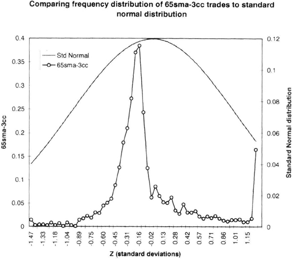
Figure 4.7 The distribution of 65sma-3cc is peaked more sharply than the standard normal distribution.

You can also use the maximum adverse excursion plot to set profit targets for scaling out of large positions. For example, if you were trading ten contracts, you could sell some at each of the profit targets of $500, $1,000, $2,000 and $3,000. We continue our analysis by examining the maximum drawdown in 777 winning trades following John Sweeney (see bibliography for details). This drawdown is on an intraday basis. These trades show some loss, but were eventually closed out at a profit. The histogram (Figure 4.10) reveals several interesting insights. About 500 (64 percent) of the trades were immediately profitable, with a loss during the trade of less than –$250. Another 100 trades showed drawdowns of less than –$500.

Thus, almost 77 percent of the trades showed a loss of –$500 or less during their evolution. There were very few trades that showed losses greater than –$1,750 and then closed out at a profit. This suggests that we could set an initial stop at $1,000 and capture almost 88 percent of the winning trades. This is a realistic way to pick the point at which a mechanical initial money management stop could be placed.

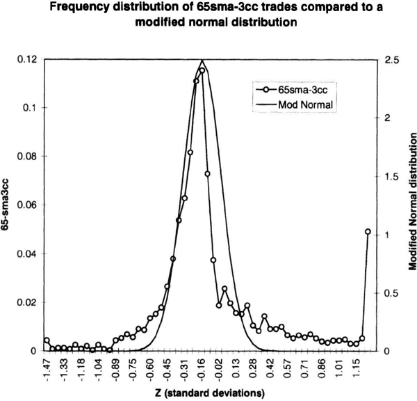
Figure 4.8 A fitted normal distribution shows that the 65sma-3cc trade distribution has “fat” tails, and falls off more quickly for small positive trades.

The same information can be viewed as a cumulative frequency chart to see how many trades achieved a certain profit target (see Figure 4.11). This type of chart shows what proportion of trades had a maximum favorable excursion of, say, $500. It shows, for example, that 50 percent of trades had reached a $1,000 profit target, and so on.

In summary, the 65sma-3cc system test over 20 years of data and 23 markets showed it is a robust and profitable system that makes money in trending periods. Since we tested the system without any initial money management stop, there were several trades with losses greater than –$3,000. We can try to clean this up by placing a stop at $1,000, as shown by the MAE plot. The detailed analysis showed several profitable trades that were closed out at a loss. We would like to minimize such trades. There were about 4 percent truly huge trades with profits in excess of $5,000. We must find an exit strategy that does not miss out on such mega-profits.

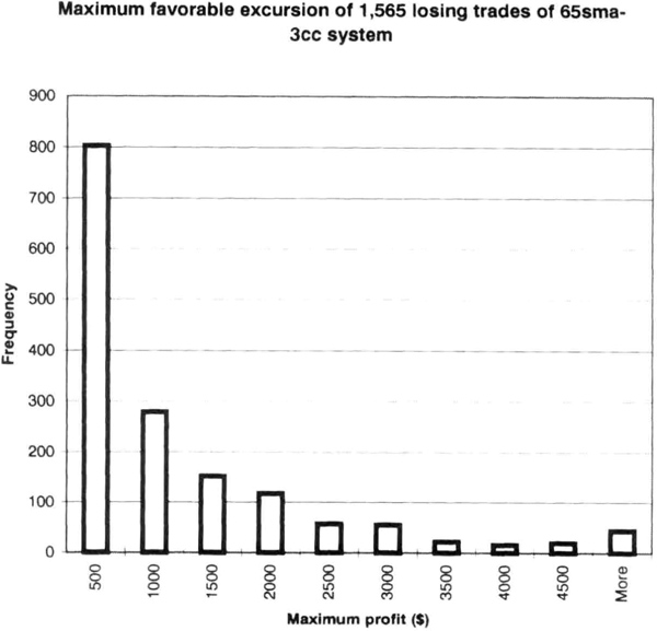
Figure 4.9 A histogram of maximum profit in 1,565 losing trades over 20 years and 23 markets from the 65sma-3cc system. This is a maximum favorable excursion plot.

Effect of Initial Money Management Stop

Since the initial test of the 65sma-3cc model was encouraging, we can now do more testing. The first item of business is to insert an initial money management stop into this model. Our detailed analysis of the MAE showed that we could safely set our stop at $1,000, or even as high as $1,750, and capture substantially all profitable trades.

However, we should insert another condition into the formulation of the model before testing for the effect of initial stops. If our stop is too “tight” during testing, we will be stopped out right after the first signal. Then, there may be a succession of trades, all in the same direction (all long or short signals), that will also result in losing trades, before one of them kicks into the major trend. Thus, the analysis would be distorted. What we want is to pick off exactly the same trades as we did without any initial stop. To achieve this goal, we must insert rules that do not allow successive trades of the same type, to ensure that we will not have two back-to-back long or short trades if we get stopped out after the first signal. In effect, with this rule, if we get stopped out, we must wait for the opposing signal before getting in. Of course, you do not need this condition for actual trading.

Figure 4.10 Analysis of 777 winning trades: maximum loss in trades that were closed out at a profit. This is also known as the maximum adverse excursion plot.

Inserting an initial condition should have two effects. (1) It should reduce the maximum intraday drawdown, since some potentially large losing trades will be cut off. (2) It should also reduce the number of profitable trades and the total paper profit, since the same stop will also cut off some potentially profitable trades. Some calculations will show if we can verify these expectations.

The results of these calculations are shown in Table 4.3, which can be compared to the results in Table 4.2. The markets and test periods are identical in both tables. Adding a $1,000 stop reduces total paper profits by 21.5 percent, from $1,386,747 to $1,088,804. Similarly, the number of winning trades fell to 689 from 810, or by 17.6 percent. As expected, the average maximum drawdown and its standard deviation also decreased, showing the desired smoothing effect due to the initial stop. The reduction was about 18.5 percent in the draw down, and 40 percent in the standard deviation. Thus, adding a hard dollar initial money management stop had the desired effect of reducing drawdown and smoothing out the variation in system performance. There was also a resultant reduction in total returns.

Figure 4.11 Cumulative frequency of maximum favorable excursion of 65sma-3cc system. Note that horizontal scale is not linear.

We chose the $1,000 initial money management stop from the MFE plot. Calculations for a $500 stop result in an even greater reduction in profits, drawdown, and volatility.

We can continue this line of thought by looking at the U.S. bond and deutsche mark markets. Our analysis of 777 profitable trades showed that once the drawdown exceeded –$1,750, few trades ended with a profit. Hence, the initial stop is varied from $250 to $1,750 in the following tests to look at the effect on the total number of profitable trades. As the initial money management stop increases, the number of profitable trades increases and then levels off (see Figure 4.12). This shows that the initial stop acts as a filter, and as the stop widens, it allows more trades to pass through. Eventually, the filter is too big, and does not cut off any trades. This allows the number of profitable trades to level off.

Table 4.3 Effect of adding a $1,000 initial money management stop to the 65sma-3cc system.

We have so far placed our stop using a dollar figure without accounting for market volatility. However, whereas in the coffee market, a $1,000 stop may seem too tight, in the corn market it may seen too wide. Thus, in some markets, a given stop will work like a stop near the left edge of Figure 4.12, and, conversely, in other markets, the same dollar stop will work like a stop on the right side of the figure.

Figure 4.12 Effect of initial money management stop on number of profitable trades. As the stop tightens, fewer and fewer profitable trades survive. The upper line is for the deutsche mark and the lower line is for the U.S. bond market.

We can get around this problem by using a volatility-based initial money management stop. For our calculations, we can set an initial money management stop as a multiple of the 15-day SMA of the daily true range for measuring volatility. We use the same continuous contracts as in Table 4.2 to test the U.S. bond market with volatility-based stops ranging from 0.25 to 3.0 times the 15-day SMA of the daily true range.

Figure 4.13 shows that a stop set at less than 1.25 times the average volatility is too tight. Once the stop increases past 2.00, the paper profit increases and the drawdown increases. The drawdown is minimized at a 1.50 stop. This means there is a balance between being too tight or too loose. The same behavior can be seen very nicely in the live hogs market (see Figure 4.14).

As might be expected, when we increase the money-management stop, the largest losing trade will probably increase. This happens because our stop is farther and farther away from the entry price. The sugar market shows this nicely (see Figure 4.15) when tested over the same period as Table 4.1. Other calculations (not shown) show that the largest winning trade is affected only a little by the initial stop, since these trades usually are profitable from the very beginning. You may set a volatility-based stop or a hard-dollar stop with equivalent results. You may have to set a different dollar stop for each market, although you could use the same volatility stop across all markets. Note that with a volatility stop, the actual dollar amount changes over time, and hence you must ensure that this stop is within your overall hard-dollar limits for risk control.

Figure 4.13 The profits (upper line) increase as the initial money management stop is loosened. Eventually, the stop is too wide and profits begin to level off. The lower line is the maximum intraday drawdown. Data are for the U.S. bond market.

You should note some limits on how the initial money-management stop can be tested. In most cases, the amount of the stop must be larger than the daily trading range. The software cannot determine if your stop could have been hit intraday if the stop is smaller than the daily trading range. Unless you have intraday data, you cannot test the effect of, say, a $250 stop using daily data.

In summary, adding an initial money-management stop is useful from a risk-control point of view because it reduces the largest losing trade and the maximum drawdown. But, it also cuts off some winning trades, and hence total profits are lower over the long term. You may add a dollar stop or a volatility-based stop, but both must follow sound guidelines.

Figure 4.14 The profits (upper line) increase as the initial money management stop is loosened. The lower line is the maximum intraday drawdown. Data are for the live hogs market.

Adding Filter to the 65sma-3cc System

So far, we have let the trading system generate pure signals without trying to filter the signals in any way. As we have seen, this system will generate many short-lived or “false” signals when a market is in a consolidation region. A filter is simply a set of rules that will try to refine the entry signals. By design, this system is always in the market. Remember that we do not have a specific exit strategy, and the long entry signal is also the short exit, and vice versa. At this stage, the goal of the filter is only to reduce some of the signals in a congestion area.

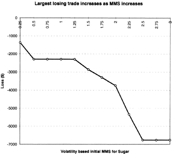
Figure 4.15 Largest losing trade for sugar using the 65sma- 3cc trading system increases as the volatility-based initial money management stop increases.

You can design many types of filters. Here we use a momentum-based filter using the range action verification index discussed earlier. The RAVI is the absolute percentage difference between the 7-day and 65-day simple moving averages of the daily close. This means that when the market is in a congestion or consolidation phase, the short (7-day) and long (65-day) moving averages tend to be close together. Conversely, when the markets are trending, these averages are far apart.

You can also use Wilder’s ADX (average directional index) as a filter for trending or nontrending markets. Specifically, if the ADX is declining, and/or below 20, then you can assume that the market is consolidating or entering a congestion phase. You could also use the x-day high-low range, or other momentum oscillators, to diagnose market conditions. Remember that any indicator you use, including the RAVI, will not work perfectly every time.

First, let us briefly review the performance of 65sma-3cc trading system in consolidating markets. As prices begin to trade in a narrow range, without a definite direction, the longer moving average (65sma) flattens out. Prices oscillate on either side of this average. Hence, you can get a succession of long and short signals as the market posts three consecutive closes above or below the 65sma.

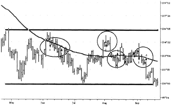
Figure 4.16 The 65sma-3cc trading system generated several entry signals as the U.S. bond market consolidated after its now-famous bear market tumble. The circled areas show the six signals—three long entries and three short entries—in this broad consolidation region.

In some sense, this becomes a self-correcting process, because the entry signals are not very far apart in price. Hence, even though you will have several losing trades in succession, the amount of the losses will be relatively small. You can imagine that in some cases the market will trade within a broad trading range, with sharp, but quick moves in both directions. The U.S. bond market has a tendency to form such consolidations. This is a worst-case scenario for the 65sma-3cc system because you will get short-lived entry signals but incur relatively large losses, since the market is making choppy moves that quickly span the trading range. Some examples of such market action follow.

Figure 4.16 shows the September 1994 U.S. bond contract consolidating after its now-famous bear market. Observe the six “false” signals from the system. Since the market was in a broad trading range, and prices were moving about on either side of the average, the false signals are inevitable given our definition of the trading system. This is a good illustration of a general principle: Whatever conditions you define, markets can always find ways to trigger false signals.

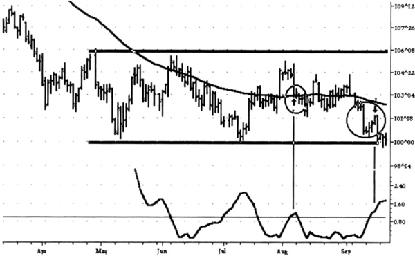
Figure 4.17 Adding a RAVI filter with barrier equal to 1.0 eliminates four of the six false trades in this broad congestion region. Notice that the 65sma-3cc model is fired only if RAVI is greater than 1 in both remaining instances.

Figure 4.17 shows the results of the same trading system with a filter. Now there are only two trades in the congestion region. The RAVI is plotted under the prices, so you can see that the signals occurred in regions where the RAVI was greater than 1. Since the model was already short coming into the picture, the first trade is a buy. The filtered model could generate a buy signal only if RAVI was greater than one and there were three consecutive closes above the 65sma.

A tight consolidation region developed immediately after the buy signal, dropping the RAVI below 1. Hence, this filtered out the next two signals, a sell and then a buy. Similarly, it also filtered out a buy signal and a sell signal in June. The last sell signal occurred when the RAVI climbed above 1 and there were three consecutive closes below the 65sma. Thus, we used the level of the RAVI to filter out some whipsaw signals.

What should be the barrier value for the RAVI to filter out signals? There is no perfect answer to this question; you will have to pick a value using one method or another. Raising the RAVI barrier to 1.5 from 1 will filter out even more trades. As Figure 4.18 shows, this model would have been short from the previous October 1993, all the way down and through two major consolidation areas, for a per contract profit of $13,696. Notice how the RAVI rose strongly above I when the trend gathered strength, peaking just before the start of the lower consolidation phase.

Figure 4.18 Increasing the RAVI filter barrier to 1.5 eliminates even more trades.

These figures illustrate that you can use a filter to reduce the number of trades from a trend-following model. You can use different filters, and for a given filter you can use different barrier levels. Note that this system still is in the market at all times: either long or short.

By now, the effects of adding a filter should be clear: (1) We filter out some false signals; (2) we can reduce the maximum intraday drawdowns; (3) we can improve the profit factor of a system, i.e., the ratio of gross profit to gross loss over the test period; (4) the average trade usually increases; and (5) the length of the average winning trade increases. Our results will depend on how we choose the filter and its barrier level.

These comments can be supported with more data. Table 4.4 shows the results of calculations for adding a 0.5 percent RAVI filter to the 65sma-3cc model with a $1,000 initial stop and $100 deducted for slippage and commissions for 14 arbitrarily selected markets. These markets are a broad basket of softs, grains, metals, energies, currencies, and index and interest rate contracts. You can compare them to Table 4.2 for an estimate of their performance without stops or filters.

Table 4.4 Effect of adding a filter of RAVI = 0.5 to the 65sma-3cc system; filtering reduces the number of trades.

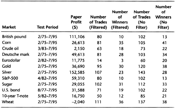
Table 4.5 shows the effect of the 0.5 percent RAVI filter on the dollar value of the average trade. The filtered system has a higher average trade, reflecting the improved quality of the entries.

Tables 4.4 and 4.5 show that as you filter a trading system, the number of trades decreases, the average trade increases, and the profit factor improves. These results are sensitive to the filtering rules. You can choose to filter a system many different ways. For example, you can use the ADX instead of the RAVI. Again, you have to make trade-offs in every choice you make.

In summary, we took the 65sma-3cc trend following system and tested its performance over 20 years of data and 23 markets. Then, we analyzed the winning and losing trades to select an initial money management stop. We filtered the system to reduce the number of signals. We used a “one-way” model, which does not allow back-to-back long or short trades. The main advantage of using a one-way model for testing is that it allows an apples-to-apples comparison of changes in trading strategy. You do not need this restriction for actual trading.

We have not tried to manage the equity curve in each of our analyses; the system was allowed to run to maximize profits. However, this system was always in the market. If we add a neutral zone, the system will not be always in the market. We can also consider adding one or more exit rules to get a smoother equity curve. With a bit of luck, the exit strategy will also create a neutral zone.

Table 4.5 Adding a filter increases the average trade.

Adding Exit Rules to the 65sma-3cc System

Selecting general and powerful exit rules is a difficult challenge in system design because the markets exhibit many different price patterns. One form of exit that is particularly easy to implement is the initial money-management stop. If the stop is hit, you exit the trade, no questions asked. However, taking profits is another matter, since you must design reentry rules should the trade continue on after meeting your exit criteria.

In the 65sma-3cc system, the approach of using entry rules as exit rules does catch long trends, but at the cost of wide swings in account equity. Hence, including exit rules tends to smooth out the equity curve. If possible, you should trade multiple contracts in each market, assigning one or more contracts to each exit rule. This allows you the luxury of not having only one “best” exit strategy.

As an alternative to the entry-triggers-exits approach, you can consider many exit strategies. One simple rule is to use a fixed-dollar trailing stop. In this case, you will set a stop, say, $1,500 away from the point of highest equity in the trade. Instead of a fixed-dollar stop, you can use a volatility-based stop, which sets a stop some multiple of the true-range away from the point of highest trade equity. Yet another exit strategy is to use a time-based stop, such as the price extremes of the last n-days. Another effective exit strategy is to exit on the close of the n-th day in the trade. For example, you could exit on the close of the fifth day in the trade. This approach works nicely if you can trade multiple contracts, and arrange to close trade from say the fifth through the twenty-fifth day in the trade.

Table 4.6 Effect of adding an exit on number of days in the market.

If you use exit strategies without an effective reentry strategy, you will miss significant moves. Hence, it makes little sense to use a trend-following strategy and then to cut off trades with a sensitive exit strategy. Exit strategies offer many opportunities for discretionary approaches. Hence, if you wish to use discretion, exit strategies are a good place to focus your attention.

An example of the effect of adding a 14-day exit to our 65sma-3cc model run with a 0.5 percent RAVI filter and a $1,000 initial money-management stop is shown in Table 4.6. The trailing exit closes out a trade if prices exceed the previous 14-day range. For example, if long, we would exit a trade tomorrow on the open if today’s close is lower than the lowest low of the last 14 days. This is a trend-following exit that should get you out near the end of a major trend, with the criterion being a 14-day reversal in prices.

Adding an exit condition decreased the days in market by 45 percent on average. At the same time, you can confirm that the profitability and maximum drawdown decreased also. Any investments you make in money market instruments during the time that the system is out of the market will add to your total return. Thus, as you make the model more restrictive, the overall profitability is restricted also. Your choice in this case is governed by your preference for a smooth equity curve versus growth in equity.

Channel Breakout–Pullback Pattern

This section discusses a trading system based on a pattern observed in mature markets, that is, markets with a large volume of institutional activity. In these markets, the big players have a tendency to fade market moves. Thus, they will resist advances and support declines. For example, when a market makes a new 20-day high, many big players will short it heavily, and push the market back into the previous consolidation. If the fundamental forces underlying the market are strong, the up trend will resume after a brief consolidation. A trading system that trades the long side only, by going long during the pull-back after new 20-day highs, is called the channel breakout–pullback (CB-PB) system.

We begin with a few examples of how the CB-PB system works, and show the actual code used for the tests. Next, we test the basic CB-PB entry strategy across 22 markets to illustrate the general validity of the idea. Then, we discuss three different exit strategies to show how you can convert the same entry strategy into vastly different trading systems. These systems vary from a short-term system, which is in the market for 7 to 9 days, to a long-term trend-following system. We will also explore the effect of using a $1,500 “close” initial stop versus a $5,000 “wide” stop. The analysis focuses on the following mature markets: coffee, Eurodollar, Japanese yen, Swiss franc, S&P-500, 10-year T-Note, and the U.S. bond.

The channel breakout-pullback pattern is for long trades only. The assumptions underlying this system are:

1. The market will begin an uptrend after the consolidation ends, because it has recently made a new 20-day high.
2. The entry during the consolidation is a low-risk entry point.
3. Exits could be placed at the nearby 20-day high, by using trailing stops, or by exiting after x-days in the trade.

The reality is that markets may have an extended consolidation after making a new 20-day high, or could even make new 20-day lows. Hence, a bias to the long side may be correct only 50 to 70 percent of the time. It is also difficult to find consistent exits, since the markets do not follow the same script every time. Hence, another difficulty with the CB-PB system is finding a consistent exit strategy. A third area of difficulty is where to place the initial stop. If the market rolls over and starts a new downtrend, then an initial stop is critical for risk management and loss control, whether it is a simple-dollar stop or a volatility-based stop.

The first example of the CB-PB pattern uses the March 1995 deutsche mark contract. Figure 4.19 shows the daily bars and, superimposed on the bars, the 20-bar trading range. The 20-day range lines have a 13-tick barrier added to both the lines to filter out some false breakouts. The chart shows that the deutsche mark broke above its 20-day range in December 1995 and then consolidated for 7 days before moving higher. Upon moving higher, it made a higher high, and consolidated again.

Figure 4.19 The deutsche mark pulls back after making a new 20-day high. The goal is to buy after the pullback. The 20-day price channel is shown for visual reference.

Ideally, we would like to buy some time during the pullback, but we do not know how long the pullback will last. Hence, the problem is how to specify that a pullback has occurred. During the pullback, markets often also make new 5-day lows. Hence, we can define this breakout and pullback long entry rule as follows: the market must make a new 20-day high, and then define a 5-day low in the next 7 days. Once it forms a 5-day low, buy on the open the next trading day. These choices are arbitrary, and you can experiment with these numbers. For example, we can buy on the close instead of on the open after the market forms a 5-day low following a 20-day high.

We now need an exit condition to evaluate this entry rule. To keep it simple, we will exit on the close of the n-th day in the trade, with n = 5 for short-term systems and n = 50 for intermediate systems. Again, these numerical values are arbitrary. You may try other values, such as a 3-day low instead of a 5-day low.

Using the Omega Research TradeStation Power Editor™, the rule appears, in part, as:

Input: Xdays (14);
  If Highest Bar(High, 20)[1] < 7 and Low < Lowest
    (Low, 5)[1]
  then buy tomorrow on the open;
  If BarsSinceEntry = Xdays then exitlong at the close;

The first line defines “Xdays” as an input-variable with a default value of 14 days. You can change this value during testing. The Highest Bar function returns the number of bars (trading days) since the 20-day highest high. The second line first checks if 7 or fewer days have elapsed since the new 20-day high. Then, it checks if today’s low is lower than the previous 5-day low (i.e., a new 5-day low). If both conditions are true, then you can buy tomorrow on the open. By default, this system will buy one contract. The third line is the exit condition, which says that if today is the x-th day since entry, then exit the long trade at the market on the close. This system will fill the long trade at the opening price of the entry day, and at the closing price of the exit day.

There is a quirk in how the Highest Bar function works. The function counts 20 days back from the day it is testing. Hence, the function will occasionally give a signal that does not work off the highest high as intended. Hence, to accurately pick off the highest high of the last 20 days, the rule should say Highest Bar(High,27)[1]. However, the difference in the results over the long run is insignificant.

Figure 4.20 shows that the March 1995 deutsche mark chart with a 14-day exit worked well. The first breakout occurred on December 28, 1994, and the pullback entry occurred on January 9, 1995, at the open of 64.11, which was the exact low of the ensuing 14 days. The exit was on the close of January 30, 1995, at 66.52, for a profit of $2,913, after allowing $100 for slippage and commissions. The next entry occurred on February 1, 1995, on the open at 65.65. The low of the trade occurred four days later at 65.07, for a 58-tick risk of $725. The exit was on the close of February 23, 1995, at 68.19. The nominal profit was $3,075.

Figure 4.20 The CP-PB strategy gave good trades with low-risk entry points.

Thus, the CB-PB system generated low-risk entries into an emerging up trend in the March 1995 deutsche mark contract. The exit on the 14th day was a lucky choice for this chart. You could use a number based on your individual preference just as well.

Note here that we specified a generic entry pattern with no specific assumptions about DM price patterns. The exit was again arbitrary. Of course, if you had exited on the fifth-day close instead of the fourteenth-day close, the profits would have been smaller. Note that the CB-PB pattern offers a relatively low-risk entry method. You can use it as a short-term system or a long-term system by simply varying the exit strategy.

So far, the exit strategy has been trend-following in nature, with some variation based on the actual day of the exit. For example, we could vary the exit from 5 days to 50 days and get completely different results. However, we will never make the “perfect” choice of x days. We can anticipate market action in a different way that does not use time as the exit signal. Instead, we will use a price we already know. Since we are buying a pullback, it is plausible to assume that the market will retest the recent 20-day high. Hence, we can write an exit signal that buys the pullback and exits the retest of the recent high. Here is how we would write the new system variation in TradeStation™:

If Highest Bar(High, 20)[1] < 7 and Low < Lowest
     (Low, 5)[1]
  then buy tomorrow on the open;
  Exitlong at highest(h, 20)[1] limit;

The first line of the CB-PB rule is exactly the same as before. The second line specifies a long exit for tomorrow with a limit order at the most recent 20-day high. This turned out to be the “perfect” model for the December 1995 S&P-500 contract. There were 12 winning trades in a row, with a total profit of $50,000 (see Figure 4.21).

The noteworthy feature here is that we started with the DM contract, using very general price patterns, and arrived at an intriguing short-term system, which performs particularly well in choppy up-trends. We made no contract-specific assumptions, and captured a general market behavior that we can expect to see in every market in the future. The CB-PB entry with an exit at a recent high works well in consolidations.

Another exit strategy involves a trailing stop, but one that will not cut off long trends prematurely. Hence, we will exit at the lowest low of the last 40 days. This will convert CB-PB into a long-term trend-following system.

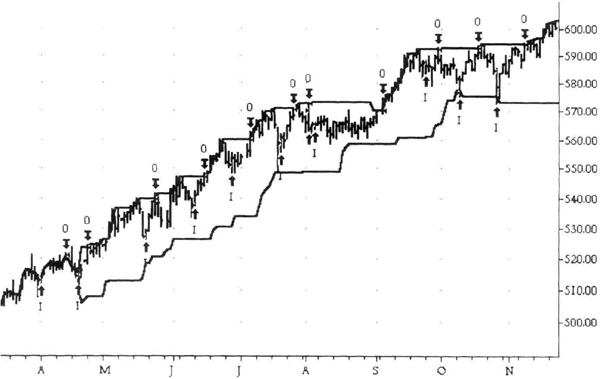
Figure 4.21 The CP-PB model with exit at the recent 20-day high using limit orders produced 12 winning trades in a row for a nominal profit of $50,000.

If Highest Bar(High, 20)[1] < 7 and Low < Lowest
    <Low. 5)[1]
  then buy tomorrow on the open;
  exitlong at lowest(low, 40)[1] - 1 point stop;

The CB-PB entry rule remains intact. The second line exits on a stop set one tick below the trailing 40-bar (trading days) low. You can see that this will become a trend-following exit. Our initial stop will close out our trade should the market head lower. The trailing stop at the 40-bar low will keep us in the trade through minor consolidations.

Notice how we took an intuitive understanding of a market pattern and adapted it to three different exit philosophies to meet specific trading preferences. Remember you could use it as a short term system by exiting at the recent high. You could exit on the close of the n-th day in the trade, for short- or intermediate-term trading. Or you could use a trailing stop. Each exit produces a trading system with different characteristics off the same entry signal. These are the types of modifications you should consider as you look at trading systems. Figure 4.22 from the March 1995 U.S. bond market will help you visualize the three exit strategies.

Now let us take a closer look at the entry signal, to see if it is any better than a random entry system. Following the suggestion of Le Beau and Lucas (see bibliography), we will try to isolate the effect of this CB-PB entry signal.

Figure 4.22 The CB-PB gave a low risk entry into the new trend for the March 1995 U.S. bond contract.

We test the CB-PB entry signal with exit on the close of the n-th day (n = 5, 10, 15, and 20), without stops and assuming no slippage or commission costs. Le Beau and Lucas suggest that if the entry signal is performing better than a random system, it should result in at least 55 percent profitable trades over a range of markets. They tested only 6 years of data and 6 markets to measure a signal’s ability to perform better than random. Here we use 22 markets and continuous contracts using all available data from January 1, 1975, through July 10, 1995. This should be a severe test of this entry signal, and our goal is to check if it is consistently profitable more than 55 percent of the time.

Table 4.7 shows that about 55 percent of all CB-PB entries were profitable. Hence, you can be reasonably confident that the CB-PB entry signal provides better than random entries. You can now marry this entry signal to a variety of risk control and exit strategies to fashion a trading system that fits your trading mentality.

The first exit strategy is simply to exit on the close of the n-th day in the trade. You are making the working assumption that the market is going to trend after the entry signal. Hence, consider now the CB-PB entry using continuous contracts, $1,500 initial stop, and allowing $100 for commissions and slippage. As discussed at the beginning of this section, we are focusing on “mature” markets. Let us consider the case when we exit the long trade on the close of the fifth day. The test uses all available data from January 1, 1975, through July 10, 1995.

Table 4.7 Percent winning trades for CB-PB entry signal calculated over all available data from January 1, 1975, through July 10, 1995.

The results of exiting on the fifth day of the trade are not impressive (see Table 4.8). Since we are buying the markets during a consolidation, most of them have not done much in the 5 days after entry. Hence, we should consider holding on to the long trade for a little while longer.

Consider what happens if we hold the long position for 50 days, exiting on the close. The conditions for the test are identical to those for Table 4.8. Table 4.9 shows there is a dramatic improvement in performance with n = 50 days. The average profit per market has increased three-fold, and the profit factor is up 46 percent. Thus, our basic assumption that the market will trend after the consolidation seems to work well about 39 percent of the time on these markets. Thus, we have converted our anemic short-term system into an interesting intermediate term system by exiting on the close of the fiftieth day.

We have previously stated that the initial stop should depend on market volatility. For example, the $1,500 stop may be “too close” given the volatility of the S&P-500 market. For the CB-PB system with exit on the 50th day using a $5,000 initial stop instead of the $1,500 initial stop, the profits dropped for all markets in Table 4.9 except S&P-500. Profits for S&P-500 increased to $141,840 on just 55 trades with 56 percent winners, a $2,579 average trade. The maximum drawdown was –$24,795, with the profit factor increasing to 2.29 from 1.62. Hence, the initial stop will influence overall system performance.

Table 4.8 CB-PB long trades with exit on the 5th day using $1,500 initial stop, tested on all available data from January 1, 1975, through July 10, 1995.

Table 4.9 CB-PB long trades with exit on the fiftieth day, using $1,500 initial stop, tested on all available data from January 1, 1975, through July 10, 1995.

Table 4.10 CB-PB long trades with exit on a trailing stop at the 40-day low, using $1,500 initial stop, tested on all available data from January 1, 1975, through July 10, 1995.

We can continue to explore the long-term nature of this entry by using a trailing stop. We know from Table 4.9 that we should use a trailing stop that will allow trends to develop. Hence, let us arbitrarily specify an exit on the lowest low of the last 40 days; this should convert the intermediate system into a long-term trading system. As before, we will use $1,500 initial stop and allow $100 slippage and commissions.

Table 4.10 shows the long-term performance of this entry with a profit factor of nearly 3 and an average trade of $1,082. The ratio of net profits to drawdown is more than 4.5. These numbers suggest that you can take the same entry and make it into a strong long-term trend-following system.

Let us now take the CB-PB entry and attach it to an exit at the recent 20-day high. It is reasonable to assume that the market will retest the recent 20-day highs as part of the backing and filling during the consolidation. Table 4.11 summarizes the test results using a $1,500 initial stop and a $100 allowance for slippage and commissions.

The CB-PB system with an exit at the recent 20-day high was interesting only on the Eurodollar, S&P-500, 10-year T-note, and U.S. bond markets. The large proportion of winning trades makes this exit particularly attractive. Notice that the length of the average winning trade was only 9 days.

You can develop other variations of this strategy. For example, one of the design features of the CB-PB system is that we want a low risk entry point into long trades. Hence, you can use a multicontract trading strategy to improve performance. Another approach would be to add a filter to reduce the number of trades.

Thus, the CB-PB system has a flexible entry to suit many trading styles. The CB-PB strategy is more profitable with an intermediate to long-term trading strategy. A short-term approach worked on a few active markets. Note also how we can develop different systems from the same entry signal by changing the exit strategy.

Table 4.11 CB-PB long trades with exit at the recent 20-day highs on a limit, using $1,500 initial stop, tested on all available data from January 1, 1975, through July 10, 1995.

An ADX Burst Trend-Seeking System

We have assumed that the market was about to trend in both the 65sma-3cc and the CB-PB systems, although we did not actually verify that the market was trending because it is difficult to measure trendiness consistently. As was shown in the discussion in Chapter 3 on the range action verification index, market momentum is often a good measure of trendiness. Unfortunately, a certain amount of smoothing is essential to minimize noise in the indicator, and this smoothing usually causes undesirable lags in indicator response.

Figure 4.23 shows the March 1993 U.S. T-bond contract trending upward nicely from December 1992 through March 1993. The indicator under the daily bars is the 18-day average directional index. ADX measures the amount of activity outside the previous bar over a given period; a strong trend usually leads to a rising ADX line. An ADX reading above 20 is considered to indicate a trend, but the ADX is a lagging indicator, and there is little significance to any particular indicator value.

ADX is closely related to double-smoothed absolute momentum, and hence will often have quirky lags. The ADX will often seem to be late in signaling a trend, and choppy markets will not follow through in the original direction that caused the ADX to rise. In fact, the market can reverse strongly, and the ADX will keep on rising.

Figure 4.23 A rising 18-day ADX can be a good indicator of a trending market.

During a strong trend, as markets make big daily moves in the direction of the trend, the daily ADX momentum can “pop” over 1.0 point, an ADX “burst.” Figure 4.24 shows the March 1993 U.S. bond contract with the histogram of the ADX burst superimposed on the 18-day ADX line. As the trend accelerates, the daily ADX changes are more than 1, and you can see relatively large bars associated with this ADX burst activity. Now you can build a trading system using this idea as shown in Figure 4.25, where the entries are circled.

Obviously, the ADX burst indicates accelerating momentum. So, here the design philosophy has changed to begin with a check that increases the odds of success of a trend-following strategy. Notice that the ADX burst is itself triggering the trade, and that the ADX is not acting as a filter. For reference, you can look up a similar system in Lucas and Le Beau (see bibliography for reference). Our goal is to take the trade in the direction of the short-term trend. If the 3-day SMA is greater than the 12-day SMA, then the trend is up, and vice versa. Table 4.12 shows the results using a simple 20-day exit strategy and allowing $100 for slippage and commissions, over all available data from Janury 1, 1975, through July 10, 1995.

The rather large profit factor suggests that the entries are effective in identifying profitable trades, so that an ADX burst is a good entry into strong trends. The profit factor is overestimated here to some degree because we are using continuous contract data. The results can be improved with multiple contracts, and you can try a variety of other exit strategies.

Figure 4.24 The histogram of ADX burst momentum shows daily changes greater than 1.

Figure 4.25 A trading system triggered by ADX burst with daily momentum changes more than 1.

Table 4.12 ADX burst system performance with $5,000 initial stop.

If you compare the number of trades here to that for the 65sma-3cc system, you will find that you have fewer entries, suggesting that the ADX burst is working as both a trade filter and a trigger. For example, this system was in the market about 3 5 to 45 percent of the time, indicating it has a rather large “neutral zone.” A trading system with a neutral zone is out of the market unless it rises above stiff entry barriers. The 65sma-3cc system is always in the market, and is a reversal-type system, whereas the ADX burst system steps aside 55 to 65 percent of the time.

We used a wide initial stop of $5,000 in these calculations to isolate the performance of the system. Table 4.13 includes performance data on selected markets with an initial stop of $1,500. The performance with the two different initial stops was generally similar.

One of the quirks of the ADX burst system is that it will often get in late, near the tops or bottoms of short but swift moves (see Figure 4.26). Such moves fire its entry signals, but the capricious market fails to follow through with a trend in the advertised direction. Hence, you should always trade a system such as this one with a preplaced stop loss order.

Table 4.13 ADX burst system performance with a $1,500 initial stop.

In summary, the ADX burst system provides entries into strong trends. It tests well across many markets and over long time periods. The system has a large neutral zone, so it is in the market only 35 to 45 percent of the time. It differs from the 65sma-3cc system, which is always in the market, and does not have a trend filter. You can use it to enter trades or increase the position in those markets. You can derive other variations using different values of the ADX burst, the look-back period for the burst calculations, and other exit strategies.

Figure 4.26 The June 1990 U.S. bond contract sells off beyond a trading range to make a new low with good momentum. The system kicks in with a short. The bond market soon reverses, to get back into the prior consolidation region.

A Trend-Antitrend Trading System

In this section we explore the trend-antitrend (T-AT) system, designed to switch automatically between an antitrend mode and a trend-following mode. You will like this system if you aggressively like to fade the market, but do not mind reversing into a with-the-trend position if needed. This system shows you that trend following is not the only way to trade the markets. Many institutions and money managers, with their deep pockets, big positions, excellent execution, and low costs, usually assume the market is ranging. These sophisticated souls will be selling new highs and buying new lows. Of course, the difference is in the trading time frames: They are in and out a dozen times, before most of us are warming up to the trade.

The challenge in this type of system is to find a consistent basis to define when to trade with the trend and when to fade it. Markets will often make new 25-day highs or lows, but without strong momentum. This can be interpreted to mean that the market is likely to reverse, so we should try to sell the highs and buy the lows. However, if the market then goes on to make news highs or lows with increasing momentum, we must immediately reverse into a trend-following position.

For this system, we will use the 18-day ADX to measure market trendiness, and an 18-day SMA of the ADX as the reference. If the ADX is above its own 18-day SMA, then the market is trending, and we will buy new highs, and sell new lows. Conversely, if the ADX is below its 18-day SMA, we will sell new highs, and buy new lows. Since we will be going against the short-term trend, we must use an initial risk control stop, or the losses will be unbearable.

We must also decide how to enter the trade. For simplicity, we will enter on the open of the next trading day. We can use the usual 20-day exit to check on the trend-following aspects. Again, for simplicity, we will test this system without specific exits, so that the entries also serve as the exit for the opposite position.

You can see how this trading system works in Figure 4.27 from the September 1993 U.S. bond contract. The market formed a base during a congestion phase, and then rallied strongly, experiencing one brief sideways period. Observe how the model readily fades new highs, and then quickly reverses in the direction of the trend. This system picked off the top and bottom cleanly during the consolidation in April and May. It was long coming into the rally off the May bottom. It hiccuped twice, in June and August, but quickly returned to the underlying long trend.

Figure 4.27 The trend-antitrend system in action on the September 1993 U.S. bond contract. Notice how it picked off turning points nicely during the consolidation. It detected two turning points during the uptrend, but quickly reversed to follow the up move.

As Figure 4.27 shows, the T-AT system caught some turning points very well. This system will also see turning points that turn out to be insignificant, and, of course, there will be some turning points that it will not notice at all. The drawback of the T-AT system is the potential for significant loss as it switches fruitlessly between its anti-trend and trend-following modes.

The usual T-AT system worked beautifully on the December 1985 deutsche mark contract (see Figure 4.28). The DM was defining a broad consolidation region after a down trend. Note how the T-AT system quickly reversed to long in September after a premature short signal. The subsequent market turns were timed flawlessly. This is quite remarkable for a mechanical system using a single trend-checking rule.

You must use good risk control with this system, since the market could move against the position in a vicious countermove. The June 1995 deutsche mark contract provides a good illustration of this (see Figure 4.29). The T-AT system signaled a perfect short trade within a day of the actual contract high. Then, it correctly picked off the bottom of the quick sell off. However, it rolled over to short during the brief congestion and then was short through the volatile countermove in late May. Trend-antitrend trading requires great faith in the system and rigid risk control, with the added benefit that the risk/reward ratio can be excellent.

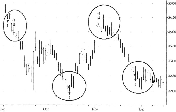
Figure 4.28 The T-AT system picked off turning points flawlessly in this December 1985 deutsche mark contract. Notice how it quickly returned to a trend-following mode in September, as the market drifted lower.

Figure 4.29 The June 1995 deutsche mark contract illustrates how the T-AT system can get trapped by a volatile countermove.

The June 1995 deutsche mark contract also illustrates the difficulty of using a heavily smoothed ADX indicator in volatile markets. The same smoothing that desensitizes ADX works against it if the market is choppy and thin.

Another quirk of the T-AT system is that it will often be slow in signaling a countermove if the market is drifting slowly, as the December 1993 cotton contract was doing near the summer top. T-AT logic correctly picked the first low (see Figure 4.30), but had to sit through the ensuing double bottom in November before the trend turned up. Once again, we have the hiccup at the start of the trend, with the system quickly reversing into the intermediate trend.

Let us briefly explore how this system was actually written, using the Power Editor from Omega Research’s TradeStation™ software. There is only one input variable, the length of the breakout period, currently set to 25 bars (days). The antitrend entry at a new 25-day high is written as follows: if today’s high was the highest high of the previous 25 days, but the 18-day ADX was below its 18-day SMA, then sell tomorrow at the market on the open. The countertrend buy signal is also similar.

Figure 4.30 The T-AT system was slow to respond to the market drift in the summer for the December 1993 cotton contract. It correctly picked the first dip of the eventual double bottom.

If high > highest (H.25)[1] and ADX(18) < average
   (adx(18), 18) then sell
  tomorrow on the open.

  If low < lowest (L, 25)[1] and ADX(18) < average
    (adx(18), 18) then buy
  tomorrow on the open.

This approach gives a symmetric long and short sell order on an antitrend basis. Let us assume you have a long position near a potential bottom. However, the market bounces up for a few days, and then reverses to begin a strong downtrend. In this situation, you want the system to switch to a short trend-following position only if it is long to begin with. Similarly, a new 25-day high with rising momentum is your signal to switch to a long position if you were short to begin with. Thus, the trend-following entries are similar to the antitrend entries, but you should first test if the system is short or long.

If MARKETPOSITION(0) = 1 and low < lowest(L.25)[1] and
     ADX(l8) >
   average(ADX(18), 18) then sell tomorrow on the open.

   If MARKETPOSITION(0) = −1 and high > highest(H, 25)[1]
     and ADX(18) >
   average(ADX(18), 18) then buy tomorrow on the open.

Here MARKETPOSITION is a special built-in function that returns 1 if the system is long, and −1 if the system is short. Once again, we have the symmetric conditions for long reentry. If we sell a new 25-day high, but the market makes new 25-day highs with increasing momentum, then the T-AT system switches to long. A similar condition holds for the short reentry.

By design, the T-AT system first tries the antitrend entry, and with-the-trend positions occur on reentry. Therefore, you should remember that this system will lose money as it hunts for a reentry market condition. Of course, if the resulting trend is a long one, then the loss at reentry will seem minor.

If you like this approach, you can try a number of variations. You could enter not on the open, but on the close or beyond the previous day’s high or low. You could also use a more sensitive reentry, as just a new 25-day high or low, not requiring the additional ADX conditions.

Table 4.14 shows the results of long-term testing on all available data from January 1, 1975 through July 10, 1995 with a $5,000 stop and allowing $100 for slippage and commissions. Only markets with positive results are included, since this strategy requires active markets.

Table 4.14 points out the strengths and weaknesses of the T-AT system. First, it does not work on all markets, and second, it generates a lot of trades. Hence, this is an expensive system to run, as shown by the drawdown numbers. The initial stop had to be rather wide, at $5,000, to allow a cushion for the antitrend component to work. However, the profit factor is healthy, as is the average trade. Hence, on mature and active markets, the T-AT system seems to work quite well. The strategy requires excellent risk control and good discipline to implement. You can now develop other variations of this system, adapting it to your trading preferences.

Figure 4.31 presents a frequency distribution of 1,311 trades generated by the T-AT system. This distribution is broader than the distribution for the 65sma-3cc system (see Figure 4.5). It also shows a spike near the $5,000 initial stop. Like the 65sma-3cc distribution, it also shows a spike for trades with big profits. Figure 4.32 shows this distribution normalized and compared to a fitted normal distribution. It is immediately clear that the T-AT trade distribution has “fat” tails compared to the normal distribution. Thus, the probability of a trade far from the center is much greater than the corresponding normal distribution. The tail on the profits side is fatter than on the losing side, suggesting that the entries are working well. Observe how the initial stop cuts off losing trades. However, there is no such cutoff on the profit side, as seen by the spike at the right edge of the distribution. This is the TOPS COLA principle introduced in Chapter 1 applied to a trading system in practice.

In summary, the T-AT system illustrates how to develop a system that automatically adjusts to market conditions. It differs from the 65sma-3cc system in that its initial stance is to take an antitrend position; the 65sma-3cc system always takes a position with the trend. A reversal condition switches the T-AT system from antitrend to a trend-following mode. The objective reversal condition assures entry in the direction of a major trend, thus allowing you to take advantage of all market conditions.

Table 4.14 Long-term performance of T-AT system over all available data from January 1, 1975 through July 10, 1995 with $5,000 stop and $100 for slippage and commissions.

Figure 4.31 Frequency distribution of T-AT trades showing a spike at the $5,000 initial stop and at trades with profit greater than $8,000.

Gold-Bond lntermarket System

This section develops intermarket trading systems for trading negatively or positively correlated markets. We begin with a quick review of the difficulties of formulating intermarket models. The gold-bond system is illustrated for negatively correlated markets and tested on other market combinations also. An example of using three markets for intermarket analysis is then given. Lastly, the gold-bond system is modified for positively correlated markets. This section will convince you that it is possible to develop interesting intermarket systems. You may have greater confidence in such systems because they contain a weak form of cause-and-effect relationships. Hence, they are often a good addition to your analytical tool set.

Figure 4.32 T-AT frequency distribution normalized and compared to a fitted normal distribution.

Many analysts have recognized intermarket relationships, which imply some form of weak cause-and-effect relationship. For example, bond prices decline when inflation is rising, and rising gold prices suggest potentially higher inflation. Therefore, we expect gold prices and bond prices to move in opposite directions (see Figure 4.33). You can also measure inflation with the prices of industrial metals such copper or aluminum. The idea is that increasing economic activity will raise the price of copper, and herald a rise in inflation. Therefore, we expect copper prices and bond prices to move in opposite directions (see Figure 4.34).

Other intermarket relationships occur with positive correlation. This means that the prices of some commodities rise and fall together. For example, rising crude oil prices suggest potential inflation, and we should expect gold prices to rise. You can use the currency markets as another good example of correlated markets. Exchange rates reflect long-term fundamental forces in the economy such as inflation and interest rates. Thus, we expect the U.S. dollar to decline at approximately the same time against other foreign currencies such as the Japanese yen and the deutsche mark. Thus, we should expect that Japanese yen and deutsche mark prices are correlated, and we should be able to generate buy or sell signals for one market from the other.

Figure 4.33 Bond (top) and gold (bottom) prices generally, but not always, move opposite one another. Thus, intermarket relationships are often imperfect.

Figure 4.34 The general inverse relationship between weekly bond (top) and copper (bottom) prices.

There are several difficulties involved with exploiting intermarket relationships. First, weak intermarket cause-and-effect relationships have time lags. Thus, the price of copper may rise for several months before bond prices begin to fall. This difference in the timing of peaks and troughs among related markets is called a time lag. The problem is that the time lags are neither constant nor consistent.

A second difficulty is that each market has its supply and demand forces, which will often distort the usual intermarket relationships. For example, we would expect copper and gold prices to move up or down at about the same time. However, there have been periods when gold and copper prices have moved in opposite directions (Figure 4.35). Thus, any systems built on intermarket forces will not be correct all the time.

A third problem is the internal technical condition of each market. Each market can become “overbought” or “oversold” at different times. The usual intermarket trends are broad trends, which could unfold over many months. Hence very short term trends in the markets can move opposite the cause-and effect relationship. Such movements can complicate your entry signals because they can trigger a risk control exit without changing the underlying trend.

Figure 4.35 An example of copper and gold prices moving in opposite directions in late 1994-early 1995.

All these issues influence the precise form of relationship you select for your system. You must also decide if you want to relate two markets or more than two markets.

The gold-bond system, which assumes that bond prices move in the opposite direction of gold prices, is a simple but effective example of how to construct an intermarket trading system. The system assumes that rising gold prices signal potential inflation and thus influence the bond market. We will use a dual moving-average crossover system, using arbitrary 10-day and 50-day simple moving averages to build the system. Here are the rules:

1. If the 10-day SMA of gold crosses above the 50-day SMA, then sell the T-bond futures tomorrow on the open.
2. Conversely, if the 10-day SMA gold crosses under the 50-day SMA, then buy the T-bond futures tomorrow on the open.

These rules say that an upside crossover of the moving averages signals rising gold prices and therefore predicts falling bond prices. Here we have not used any filters for the emerging trend in the gold market, but you could certainly use the ADX indicator. To use the ADX filter, simply require that the 14-day ADX be rising, and determine the direction of the short-term trend by comparing the 3-day SMA to the 20-day SMA. The specific rules for the ADX-filtered system are as follows:

1. If the 14-day ADX is greater than its value 14 days ago, and if the 3-day SMA is below the 20-day SMA of the daily gold closes, then buy the bond futures on tomorrow’s open.
2. Similarly, if the 14-day ADX is above its value 14 days ago, and the 3-day SMA is above the 20-day SMA of daily gold closes, then sell the bond futures on tomorrow’s open.

We tested both of these models on U.S. bond and Comex Gold continuous contracts from August 23, 1977, through July 1, 1995, with an initial $5,000 money management stop and $100 allowed for slippage and commissions. As discussed above, the short-term trends in the markets can be a problem for trade entry. The results are summarized in Table 4.15.

These results suggest that there is indeed a broad inverse relationship between gold and bond prices. However, from a trading perspective, only about half the signals are profitable. The filtered gold-bond system was significantly more profitable than the dual moving average crossover system, with about half the maximum drawdown. The gold-bond system could function as a filter to check whether the “trading environment” favors rising bond prices.

Table 4.15 Results of testing the gold-bond systems, August 21, 1977 through July 10, 1995.

We know that there are lags between the price movements among markets. Since a hint of inflation can move many other markets, we should check out the basic gold-bond system on other market combinations, such as the soybeans-bond, copper-bond and deutsche mark-bond combinations. The grain markets often signal inflation, and the soybeans market is used as a proxy for those markets. The copper market follows strength in the industrial sector and is a leading indicator of inflation. Lastly, interest rates signal broad forces in the economy that also influence the currency markets, such as the deutsche mark. We used the gold-bond system for negatively correlated markets with the same $5,000 initial stop, one contract per trade, and $100 for slippage and commissions, and tried to generate buy and sell signals for the bond market from the markets indicating inflation.

The data in Table 4.16 confirm that changing trends in markets heralding inflation can be used to trade the bond market. Of all the combinations tested, the copper market seems to provide the best indication. In every case, only about half of the signals were profitable. Thus, these systems follow the well-known principle of economic forecasting: if you must forecast, forecast often.

So far, we have used only one market to develop trading signals for bonds. However, you could use more than one market to derive trading signals. We tested the use of two markets, gold and soybeans, to develop trading signals for bonds. We chose these two markets because they seemed to have unrelated supply-demand forces. We also tested the gold, copper, and bond combination for completeness.

We extended the basic gold-bond system to three markets by specifying that both gold and soybeans must be trending up or trending down at the same time to generate the opposite signal for bonds. For example, if the 10-day SMA of the daily close was below the 50-day SMA for both gold and soybeans, then that would trigger a buy signal for bonds. The results of the historical tests for the combined gold-soybeans-bond system were better than either the gold bond or soybeans-bond systems. As usual, we used a $5,000 initial stop and allowed $100 for slippage and commissions.

Table 4.16 Results of testing the gold-bond system on other market combinations.

The test results in Table 4.17 show that using three markets reduced the total number of trades, as you would expect. For example, the gold-bond tests and soybeans-bond tests produced 122 trades, whereas the gold-soybeans-bond trio produced only 77 trades. The profit factor also improves with three markets, as you would expect from improved filtering. For example, the gold-copper-bond trio had an impressive profit factor of 2.53, and produced essentially the same profits as the copper-bond combination with 35 percent fewer trades. These tests show that you could try to improve the effectiveness of intermarket systems by using three or more markets to filter out the signals. Note that as you add more markets, the effectiveness often decreases because of random noise among markets.

Table 4.17 The gold-bond system extended to three markets.

Figure 4.36 The approximate inverse price relationship between crude oil and corn.

The basic gold-bond system tries to capture the weak negative correlation between the gold and bond markets. Such correlations also exist among other markets. Most trend-following systems have tested out poorly on the crude oil market, losing more than –$40,000. A negative correlation exists between crude oil and corn (Figure 4.36), and between crude oil and short-term interest rates. The Eurodollar market can be used as a proxy for short-term interest rates. Results of tests of the gold-bond system as developed on the corn–crude oil and Eurodollar–crude oil combinations are shown in Table 4.18. These tests use trend change signals from the corn and Eurodollar markets to trade crude oil.

The results show that the gold-bond system could be used to make a small profit on the crude oil markets, if we derive our signals from the corn market or the Eurodollar market. This is a big improvement over the results for typical trend-following systems.

Thus, these results show that you can use the gold-bond system to trade weak negative correlations among markets. The negative correlation between crude oil and corn is not obvious; it may have to do with the rising costs of international shipments—as crude oil prices increase, transportation costs increase, and U.S. corn producers must pay for the higher costs by lowering corn prices. The inverse relationship between rising crude oil prices and short interest rates is through the fear of future inflation.

Table 4.18 The gold-bond system tested to trade crude oil using corn and Eurodollar markets for signals.

So far, all the intermarket systems we have discussed exploited the negative or inverse price relationships between markets. You could certainly extend these ideas to trade positively correlated markets, in which a rising trend in one market would be a buy signal in the other market. The Japanese yen–deutsche mark combination uses trend change signals in the Japanese yen market to produce signals for the deutsche mark. The corn–live hogs combination uses trend changes in corn to generate signals for live hogs. Since corn is fed to hogs, rising corn prices could increase the production costs for hogs (see Figure 4.37). To test the gold-bond system in these correlated markets, we use a $5,000 initial stop for the currency markets, but only a $1,000 initial stop for the live hog market due to its relatively low volatility. As usual, we deduct $100 for slippage and commissions (see Table 4.19).

Figure 4.37 The relationship between corn prices and live hog prices.

Table 4.19 Gold Bond system extended to correlated markets, such as JY-DM and C-LH.

In summary, these results show that you can successfully use correlated markets to generate trading signals. You may feel more comfortable with the signals from intermarket systems because there are weak cause-and-effect relationships that have stood the test of time. At a minimum, you could use intermarket analysis to develop “background” information that could be used as input into your money-management algorithm. For example, an intermarket system signal could be used to increase the size of existing positions or put on new ones. You could also use an intermarket signal as an exit strategy for conventional single-market systems.

A Pattern for Bottom-Fishing

Market-specific systems work best on a particular market because they capture some unusual feature of that market. It is difficult to speculate why certain markets show signature patterns. We should take extra care when developing such systems because the market mechanics driving such patterns could change abruptly.

The S&P-500 futures contract can be used to illustrate a pattern-based approach. For instance, we consider a continuous contract from April 21, 1982 through July 10, 1995, and test the standard simple moving average crossover system with 10-day and 11-day simple moving averages. We use a relatively loose $2,000 initial stop, which will absorb random price fluctuations, and allow $100 for slippage and commissions.

The 10- and 11-day dual crossover system lost $181,005 on paper, with 530 trades. Only 34 percent or 178 trades, were profitable, with a maximum intraday drawdown of $189,370. One interesting feature was that virtually all the loss ($185,545) was on short trades. This makes sense if we recognize that the market has been generally moving up since 1982. However, it is striking that this simple trend-following system fared poorly in spite of the prolonged up-trend. So the S&P-500 futures market is not a trend-follower’s delight.

Because all of the losses were on the short side in the previous test, it makes sense to try the simple moving crossover system in the antitrend mode. The antitrend rules are as follows:

1. Buy if the 10-day SMA crosses below the 11-day SMA on the close.
2. Sell if the 10-day SMA crosses above the 11-day SMA on the close.

Using the same test period, initial stop, and allowance for slippage and commissions as the previous test, the turnaround in profits with the antitrend rules was remarkable. This antitrend 10- and 11-day system netted $55,920 for a swing of $240,925 on 531 trades. Fully 48 percent, or 254 trades, were profitable, with a maximum intraday drawdown of $32,735.

The results of the antitrend approach are not spectacular. However, they do highlight the unusual nature of the S&P-500 market. They suggest that you could find market-specific systems that would test poorly on other markets. For example, the 10/11 antitrend strategy lost $56,775 when tested on the Swiss franc continuous contract over the same period, but the 10/11 trend-following strategy lost just $13,088 over the same period.

The following is a glaring example of how “hindsight” influences system design. There were many “V” bottoms on the daily bar-charts of the S&P-500 market, so a bottom-fishing strategy that tries to pick bottoms was attempted. Theoretically, it should test well since this is an antitrend approach. The rules for the S&P-500 “bottom fishing” pattern are as follows:

1. A 20-day low has formed within the last 5 days.
2. Today’s high-low range > X; X = 4 for conservative trades; X = 1 for aggressive trades (each point is not one tick, but one full S&P index point = $500)
3. Today’s closing-opening range > Y; Y = 3 for conservative trades; Y = 0 for aggressive trades.
4. If rules 1, 2, and 3 are true, then buy tomorrow on the close.
5. Exit on the close of the twentieth day in the trade.
6. Initial money management stop = $2,000 per contract.

Table 4.20 Performance of bottom-fishing system with $2,000 initial stop and exit on the close of the twentieth day in the trade using actual S&P-500 data with rollover.

Note that we can fully automate the bottom-fishing pattern. We have no difficulty getting entries, because if we get a signal today, we can buy on tomorrow’s close. So it is easy to implement using a mechanical system. For example, the analysis can be done after market hours, and the order entered before trading begins.

This system has a conservative entry combination and an aggressive entry combination. The conservative approach generates fewer trades. You can modify this pattern in many ways. The most obvious change is the exit strategy. For example, you could set an exit target at the most recent 20-day high.

The system was tested using System Writer Plus™ and actual S&P-500 contracts. The rollover date was the twentieth day of the month before expiration. The results are in two blocks in Table 4.20 because System Writer can process only 30 contracts at a time. You can treat either the conservative or the aggressive set of X and Y values as an unoptimized set. Both combinations were profitable on both blocks of data.

The equity curves for both options are shown in Figures 4.38 and 4.39. The equity curve for the conservative option is smoother than the aggressive option. Also, the aggressive option can produce larger drawdowns than the conservative values.

Data using the March, 1995 S&P-500 contract yield Figure 4.40, for X = 4 and Y = 3, and Figure 4.41 is for X = 1 and Y = 0. This system picked off the bottoms very accurately. Entry and reduced slippage are assured by entering and exiting on the close. Thus, a pattern-based, antitrend, bottom-fishing approach works nicely on the S&P-500 market.

You can try a variety of exit strategies. Instead of an exit on the close of the twentieth day (case 1), use a trailing stop on the 5-day low after a $1,000 profit on the trade (case 2). Case 2 with X = 4, Y = 3, a $2,000 initial stop, and $100 for slippage and commissions from February 12, 1988 through July 10, 1995, had a profit of $59,025 over 44 trades (45 percent winners) with a drawdown of –$7,625. You can compare these data to the second row in Table 4.20 (case 1). Thus, the new exit strategy produced approximately the same profits, but with a smaller drawdown and more winners. The equity curves for case 1 and case 2 are shown in Figure 4.42. You can see that case 2 has shallower drawdowns than case 1.

To check the basic validity of the bottom-fishing pattern on other markets, we must modify the pattern slightly to make it more general. Values of X = 0.1 and Y = 0 are chosen in order to test across many markets. A trend-following exit, at the lowest low of the last 20 days, was chosen because not all markets are as dynamic as the S&P-500 market. The entry is switched to above the high of the signal day, instead of buying at the next day’s close, to reduce the number of entries in downtrends. The initial money management stop is $2,000, and as usual, $100 is deducted for slippage and commissions. The pattern uses all available data from January 1975 through July 1995 using continuous contracts on 17 markets. The results are for trading one contract at a time.

Figure 4.38 Equity curve for bottom-fishing pattern (9/82-7/95) with X = 4 and Y = 3 (conservative trades) for S&P-500 data with rollovers. Initial money management stop was $2,000 per contract.

Figure 4.39 Equity curve for bottom-fishing pattern (9/82-7/95) with X = 1 and Y = 0 (aggressive trades) for S&P-500 data with rollovers. Initial money management stop was $2,000.

Figure 4.40 The bottom-fishing pattern with X = 4 and Y = 3 picked off the important December 1994 bottom.

The generalized bottom-fishing pattern was profitable on 11 of 17 markets, including deutsche mark, Eurodollar, gold, Japanese yen, coffee, orange juice, Swiss franc, S&P-500, silver, 10-year T-notes, and the U.S. bond market. Thus the pattern also seems to work on markets that trend well or have good swing moves. The results are given in Table 4.21.

These data suggest that the bottom-fishing approach captures a basic trading pattern in the markets. The long test period and the profits on a variety of markets indicate that the idea is robust. The difference in performance between markets seems to be the amplitude of the movement after forming the pattern.

An extension of the test of the bottom-fishing pattern to stocks explores its performance over different time periods. Figures 4.43 (weekly) and 4.44 (monthly) illustrate how the generic bottom-fishing pattern works. Figure 4.43 has weekly data for Union Carbide showing how the pattern picked the bottoms in 1990 and 1991. The pattern also stayed long throughout the major up-trend. The pattern tests well with weekly data on stocks. Figure 4.44 has monthly data for Caterpillar Tractor. The bottom-fishing pattern responded to the 1992 bottom and stayed with the stock throughout the rally.

In summary, the bottom-fishing pattern–based system is a good example of a market-specific system. You can use it as a model to develop other pattern-based systems on the S&P-500 market. The pattern can be generalized successfully to other markets, including stocks. The bottom-fishing pattern also works across time periods such as daily, weekly, or monthly. Thus, the bottom-fishing pattern captures a fundamental pattern of price evolution.

Figure 4.41 The bottom-fishing pattern with X = 1 and Y = 0 entered the market closer to the December 1994 bottom.

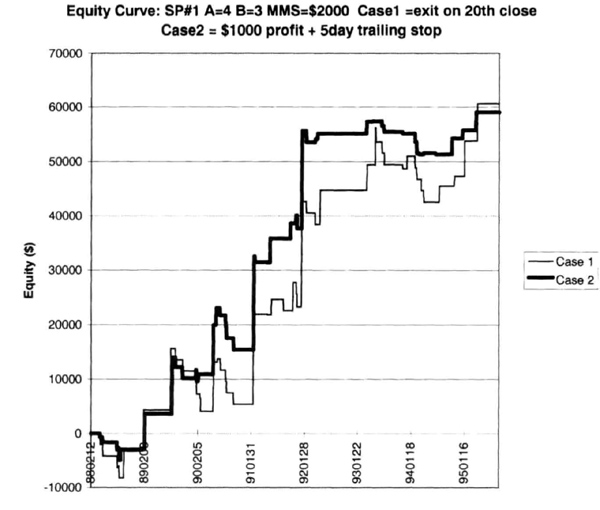
Figure 4.42 Equity curve for case 1 and case 2.

Table 4.21 Results of testing the generic bottom-fishing pattern on other markets.

Figure 4.43 Example of generic bottom-fishing pattern on weekly stock data.

Figure 4.44 Example of generic bottom-fishing pattern on monthly stock data.

Identifying Extraordinary Opportunities

Once or twice a year, the futures markets provide extraordinary opportunities for exceptional profits, and if you can take advantage of these opportunities, your account performance will improve significantly. Ideally, you should try to increase position size in markets that present extraordinary opportunities. You can use a fixed formula or discretion in arriving at the increased exposure.

Figure 4.45 of the September 1995, Japanese yen contract illustrates such an extraordinary opportunity. If you had tripled your exposure to the Japanese yen during these two awesome moves, you would have made an extra $40,000 with only moderate extra risk. These are the situations when you need “the courage to be a pig,” as one famous money manager has said.

The challenge for system design is to find a consistent definition of an extraordinary opportunity. Once you have a consistent definition, you can use it any way you wish. In particular, you can use discretionary trading to adjust your exposure to the markets to exploit these situations.

Figure 4.45 Extraordinary market opportunity identified by the 7-day SMA crossing beyond the 3 percent band around the 50-day SMA.

Figure 4.46 A market can signal extraordinary opportunities on the long and short side within a short period.

The definition of an extraordinary opportunity as used here is simple. Use a 50-day SMA and plot a 3-percent trading band around it. Then a 7-day SMA must cross outside the upper or lower band to complete the identification of extraordinary markets. Thus, if the 7-day SMA crosses above the upper 3-percent band, an upside extraordinary situation is declared (see Figure 4.45). A converse definition is applicable for bearish markets. The best scenario is that the market follows through vigorously in the direction of the established trend. The worst scenario is that the market teases you for a day or two before returning into a congestion zone. Then use an initial stop to close out the trade.

Be aware that a market can signal good opportunities for long and short trades within a few months. Some times a short-lived long signal can be a prelude to a strong down move, as the S&P-500 did in 1987 (Figure 4.46). Hence, be alert when you get the signal for an extraordinary market condition.

The next major challenge is an exit strategy. A simple strategy of exiting on the close of the twentieth day in the trade works well. Another exit strategy is to close out the trade when the 7-day SMA moves back inside the trading bands. You can imagine several other exit strategies, and I encourage you to test them all.

Table 4.22 summarizes a test for the extraordinary opportunity idea on all available data for several markets from January 1, 1975, through June 30, 1995. These calculations combined the usual 20-day channel breakout with the rules for declaring an extraordinary market opportunity. The long entry rule requires that the 7-day SMA be beyond 1.03 times the 50-day SMA in order to purchase just above the highest high of the last 20 days. The opposite conditions are needed for the short trades. The exit was on the close of the twentieth day, and as usual, a $3,000 stop and $100 for slippage and commissions were used, to allow for a more accurate test.

Table 4.22 Performance summary with 3-percent trading band, exit on close of twentieth day in trade.

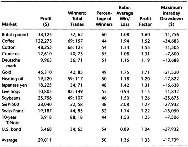
The long test period (20 years in some cases), the wide diversity of markets, and the relatively high proportion of winning trades suggests this strategy is a valid approach toward identifying extraordinary market opportunities. The MIDD numbers suggest that the exit strategy is critical to the success of this system. As an example, the results of adding a trailing stop and narrowing the bands are shown in Table 4.23.

In our discussion of risk of ruin, we assumed the following constant parameters: probability of winning, payoff ratio, and fraction committed to trading. However, in actual trading, the probability of winning and payoff ratio change with time. Hence, you should consider changing your fraction of capital risked on a trade, especially if an extraordinary market opportunity is recognized.

Table 4.23 Performance results with 1 percent trading band and trailing 20-day stop.

The test results in this chapter are with just one contract; this is an opportunity to use discretion and increase your exposure to the markets. Hence, the potential impact on returns can be quite significant with multiple contracts, based on the one-contract results shown here. You also have the option of using discretionary exits, or other exits based on shorter term data, such as an hourly chart.

Remember that you can check fundamental developments to confirm the presence of extraordinary market conditions. For example, there may be an unusual weather pattern, a political development, or a crop failure, to name just a few of the types of events you can read about in the financial press. In a purely technical sense, you do not need the confirmation from fundamental analysis. However, if unusual fundamental conditions exist, that may give you clues as to the probable duration and potential amplitude of possible market movements, and help you determine how you could adjust the size of your position.

Performance Update: 65sma-3cc System

A retest of the 65sma-3cc was performed on a globally diversified portfolio from January 1995 through July 2000 using a $5,000 initial risk, variable-contract trade sizing using the 50-day average true range and allowing $100 for slippage and commissions. This is a long-term trend-following system that should benefit from portfolio diversification. The portfolio is shown in Table 4.24.

Table 4.24 Globally diversified portfolio for the 65sma-3cc system.

This model is currently in the midst of a drawdown that started in September 1998 (see Figure 4.47). In addition, the current leverage is probably too high, with a monthly standard deviation of about 14 percent before interest and fees. However, the return efficiency is a respectable 0.25, in line with benchmarks discussed later in this book. The average monthly return before fees and interest was 3.45 percent, implying raw annual returns in the 50 percent range. The worst theoretical drawdown was 43 percent, in line with recent stock market declines, and about three times the standard deviation of monthly returns, also in line with the discussion to follow in Chapter 7. The calculations confirm the validity of the original model and the robust nature of basic trend-following systems that use few parameters and can be traded on a broadly diversified portfolio without changing parameters.

Figure 4.47 True out-of-sample equity curve for the 65sma-3cc system.

The 22-month length of the current drawdown has exceeded the length of all previous drawdowns but is below the theoretical projection of 33 months. It still raises concerns about the level of portfolio diversification and the slow exits of the model. The best one can hope for is a strong recovery because it is unusual to have such a long drawdown in a diversified portfolio.

ATR-Band Breakout Model

We can extend the idea of the extraordinary opportunity system by devising volatility-based bands. The simplest definition of a band breakout model is the use of breakout levels a fixed percentage above and below an intermediate to long-term moving average. These types of bands were the basis of the extraordinary opportunity system. The idea of bands can be interpreted to mean a moving barrier that can be based on any imaginable criterion. One class of such bands is that of volatility bands, in which the volatility can be measured with average true range (ATR) or the standard deviation of prices. The principal benefit of this extension is to make the bands adaptive, that is, responsive to market volatility. When the volatility is low, the breakout barrier is closer to the moving average. Conversely, near the tops and bottoms of trends, volatility is relatively higher, and the bands are farther apart.

Band breakout models share all of the benefits of breakout-style systems with the additional advantage that they adapt to the market. Such systems can be applied easily to a global portfolio. The bands can be based on any measure of price change that adapts to market action. Let us now examine bands based on average true range. We use a 50-day moving average for convenience, and build bands by averaging the daily true range over the last 50 days (ATR50). Thus, the bands are located one ATR50 range above and below the 50-day simple moving average. The long and short exits are at the 25-day simple moving average of the close because we want to avoid trading in congestions. We use two times the ATR50 and $5,000 risk to trade multiple contracts. The portfolio is composed of the major liquid markets in North America, Europe, and the Pacific Rim, covering the major sectors, such as stock indices, long and short interest rates, energies, currencies, agriculturals, and softs. Thus, we are testing a nonoptimized, prespecified system on a broadly diversified portfolio.

Figure 4.48 Equity curve for a volatility-band system, which is an extension of the extraordinary opportunity system. Note the vertical axis is drawn to show the growth in the value of a $1,000, instead of a $1,000,000, account.

The simulated equity curve with a $100 allowance for slippage and commission is shown in Figure 4.48. The average monthly return, without fees or interest, is 2.9 percent, and the standard deviation of monthly returns is 8.9 percent. This works out to a return efficiency of approximately 0.33, with a maximum drawdown of just under 20 percent (~2.25 sigma). There were 11 drawdown streaks since January 1, 1995, the average drawdown being 4 months. However, a fit of the exponential distribution to the drawdown streaks suggests a potential “worst” case drawdown length of 22 months.

These calculations show the strengths and weaknesses of breakout-style systems. These systems are robust, and many markets can be traded with the same parameters. They are vulnerable to false breakouts, and their primary resistance to drawdowns comes from portfolio diversity. However, should the correlations between markets shift, or should the major groups not have sustained trends, a prolonged drawdown will result.

Trading Stocks

All of the ideas developed so far in this chapter can be used to trade stocks. In this section, we develop and test the trend-following model on futures and stocks. We begin by discussing the strategic differences between futures and stocks as they relate to portfolio design and trading systems.

The simplest stock-trading approach is a multiyear, long only, buy-and-hold strategy. In general, it is difficult to beat a buy-and-hold strategy on stocks that are in a secular uptrend because the buy-and-hold strategy is a trend-following model without trailing stops. Thus, the buy-and-hold strategy can withstand large percentage retracements as well as long-lasting retracements (that last 12 months or more) without exiting the position. This strategy is always in the market, so you are unlikely to miss sudden, large moves in a stock you own. Note further that the buy-and-hold strategy has low transaction costs and is a tax-efficient strategy because there are no tax consequences to holding a stock with unrealized gains. One can approach the buy-and-hold stocks strategy with futures by using very slow exit strategies that will hold a position for 65 trading days of longer. However, almost by definition, a buy-and-hold strategy is impossible to execute using futures contracts because, unlike stocks, futures contracts expire according to a prespecified schedule. Thus, a buy-and-hold strategy using futures has large transaction costs and tax consequences.

Another key difference between futures and stocks is the leverage implicit in the approach. The buy-and-hold strategy is typically an unleveraged strategy, so the effect of volatility is muted when compared to futures trading. The leverage in futures necessitates profit-taking strategies (i.e., exits) that will lock in gains in a position. When any profit-taking approach is applied to trading stocks, we immediately have tax consequences, and we will often be late entering and exiting moves. Thus, for a stock-trading strategy to be successful, the choice of the stocks being traded is critical.

The trade sizing algorithms are also significantly different for futures and stocks because of the varying contract sizes and available leverage. The equity in one’s account will limit the quantity and number of stocks that can be traded. In futures, there is an extra factor: one’s account equity and the desired leverage determine the size of positions. However, the amount of cash actually required to put on positions is much larger in trading stocks. Thus, it may be easier to purchase 1,000 instead of, say, 50,000 shares of a stock because of the equity in the portfolio and liquidity considerations.

The duration of the average trade will depend on the time frames used for analysis. Monthly, weekly, and daily data can be used with stocks to follow the long-term trend. The essential choice for stocks is between weekly and daily data, with trade durations being approximately five times longer with weekly data. The more volatile a stock, the shorter the needed time frame of analysis. Hence, for technology stocks, daily data may be more relevant than weekly data. You will be closer to a buy-and-hold strategy with weekly data than with daily data because of the longer time frame for analysis.

A variety of stock selection screens can be developed to identify stocks that are in favor. It is best to trade stocks that are in leading industry groups. The new highs list, the most actives list, and the holdings of leading mutual funds are good places to find stocks that may be worth trading. Investor’s Business Daily prints a number of proprietary performance measures and offers graphical chart reviews to help identify leading stocks. Over time, different groups come into favor and go out of favor, as the “story” changes. Hence, reading the financial press will help isolate popular investment themes. The results of your trading using the same system on all stocks will be highly dependent on the stocks you choose to include in your portfolio.

The following momentum-based model uses a long-term trend-following approach on stocks in well-defined uptrends. Using this model, we want to buy when the stock is in a definable uptrend and makes new 20-day highs in price accompanied by strong momentum, as measured by the ADX indicator. We use daily prices and the 65-day simple moving average (SMA65) as references, and assume that the trend is up if the current close is above the SMA65 and the highest high of the past 20 days is also above the SMA65. We then add a condition that confirms that the stock is indeed trending higher. We use the average directional index (ADX) indicator and require that the current value of the 18-day ADX be above 20. The choice of the ADX indicator and its reference level is based on a “general rule” from futures trading. If both conditions are satisfied, then we set the entry price two-ticks above the highest 20-day high. Now a single tick is the minimum increment in which the stock trades, which may be, say, one-hundredth of a currency unit or some other value based on the exchange on which the stock is traded.

The trade sizing algorithm uses a retracement distance (“Dist”) or risk of three times the average 40-day true range (ATR40). The true range is measure of the “effective” daily price range that is popular with futures traders, and allows for gaps in prices. The true range is the difference between the true high (today’s high or yesterday’s close, whichever is higher) and the true low (today’s low or yesterday’s close, whichever is lower). The true range is a measure of the range of price action or “volatility”; the higher the ATR40, the greater the market volatility at that point in time. We convert the ATR40 into dollars (or any other currency unit) by multiplying the ATR40 by the value of 1 full point change (the so-called “BigPointValue”) in the value of the stock, usually $1 or 1 currency unit. Note that the BigPointValue can vary widely among futures contracts. We then calculate position size by dividing the equity at risk, in this case $5,000, by the dollar value of the ATR40. Note how the size varies inversely as the volatility. When prices have consolidated, volatility is relatively low and the size of the position is relatively high.

Our exit strategy is very simple: merely the trailing SMA65. This fulfills the requirement that we stay with the trending stock as long as possible. If one uses daily data, the SMA65 is relatively far away from prices and can absorb a fair amount of adverse price movement without being shaken out of position. The ability to absorb adverse movements is considerably greater with weekly data. The ADX condition tries to protect us from the scenario in which the stock is trading choppily, and the 20-day highest high is not too far from the SMA65, so that the stock repeatedly makes new 20-day highs and then retraces down to the SMA65. Thus, a secondary benefit of the ADX indicator is to proteet account equity in choppy markets. The actual Omega Research TradeStation TM software code is:

{--- Code for Omega Research TradeStation ---}
   {--- Momentum Trend System for Stocks and Futures ---}
   {--- © 2000 Tushar Chande ---}
        Inputs: Eqty(5000);
        Vars : Numlong(0), Dist(0) :

   {---- Contract calculations ---}

         Dist = 3*Average(Truerange, 40);
         {-- convert to currency units --}
         Dist = Dist*BigPointValue ;
         {-- protect division by zero --}
         If Dist > 0 then
                  Numlong = intPortion(Eqty / Dist)
         Else           Numlong = 0 ;

   {--- Entry Signals ---}

        if c > average(C, 65) and highest(h, 20)[1] >
        average(C, 65) and adx(18) > 20 then buy Numlong
        contracts at highest(h, 20) + 2 points stop;

   {---- Exit Signals ---}

         Exitlong at average(C, 65) stop;

   {--- End of Code ---}

Let us now see how this system works on stocks and futures. Figure 4.49 shows an entry into Veritas Software Corp (VRTS) stock in August 1999. Notice that the close was above the SMA65 (crosses) as was the 20-day highest high. The 18-day ADX was above its reference level of 20. Thus, VRTS met our entry conditions, and the system opened a long position at a new 20-day high in late August with a suggested size of 1,088 shares. Figure 4.50 shows how the trade evolved into 2000. The rally in technology stocks in late 1999-early 2000 carried VRTS substantially higher. The strength of the trend kept the 18-day ADX above the reference level throughout the rally. The correction in technology stocks in March 2000 caught up with VRTS, and it crashed through its SMA65, triggering an exit.

Figure 4.49 A daily chart for Veritas Software Corporation stock showing the building blocks of the system. The entry conditions are satisfied when the 18-day ADX indicator is greater than 20 and the daily close and the 20-day highest high price are both above the 65-day SMA of the close. The entry price is two-ticks above the 20-day high.

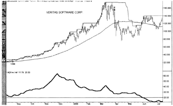
Figure 4.50 The system exits Veritas stock at the 65-day SMA of the close, shown here by the dotted line. The trend was exceptionally strong because the 18-day ADX stayed above 20 for the duration of the move.

Figure 4.51 The entry setup for the system illustrated using a continuous contract of the London IPE Brent Crude futures contract. The entries work similarly on stocks and futures—buying strength in a rising market with confirmation of trend strength.

Note how the relatively slow exit strategy did give up a significant portion of open trade equity before actually closing the position. However, this same strategy withstood several sharp corrections along the way. VRTS bottomed and made new 20-day highs in summer 2000. However, the ADX indicator was below 20, so it did not confirm the new 20-day highs, and a key entry condition of the trading system was not satisfied during the consolidation well below previous highs. The ADX stayed well above 20 during the correction in March 2000, but actually peaked in November 1999. The reason for the slow response by the ADX is the heavy smoothing built into the indicator, which is why we did not use the it to trigger exits.

Figure 4.51 shows the same strategy when trading the IPE Brent Crude contract during the rally in energy prices in 1999-2000. When the Brent Crude prices bottomed in early 1999 and rallied above the SMA65, the 18-day ADX rose also, signaling a strong trend. The system went long at a new 20-day high with four contracts per $5,000 risk in March 1999. The position was close in October 1999 at the SMA65 with more than a $32,000 profit on the trade. As the Brent Crude market continued to rise, the ADX indicator did not confirm the trend, and we avoided the ensuing consolidation. The system bought new 20-day highs in February 2000, but the increased risk led to a size of two contracts per $5,000 risk. The market retraced quickly off the highs, and that trade was a modest loser, reflecting the limitations of the exit strategy. The subsequent sell-off helped the ADX to adjust to rising prices, so that it signaled a strong rally in May 2000. Notice how the SMA65 can absorb considerable adverse price action in futures, just as it does in stocks, but needs smooth trends to lock in substantial profits. The Brent Crude example illustrates the similarity of trends in stocks and futures, and how the same technical rules can be used on both, producing similar responses during trends. Naturally, if the markets do not trend smoothly, or retrace rapidly off new highs, then this system will be unprofitable because it is not designed to react to those scenarios.

Figure 4.52 The system applied to a continuous contract of the Paris MATIF Notional Bond futures contract showing that the entry conditions can be satisfied by a stock or market without significant follow through, causing trading losses.

Figure 4.52 illustrates the scenario in which the market satisfies the entry conditions of the system but does not follow through sufficiently to be profitable. We examine the Paris MATIF Notional Bond as it rallied after a long downtrend and then continued to consolidate after putting in a bottom. Note that the ADX will often behave like a coincident indicator rather than a leading indicator because it is also derived from closing prices. Hence, a “high” value of ADX is not sufficient to signal a strong trend that persists for many weeks or months.

This system can be used to trade mutual funds using daily data in the same manner as any other stock. Figure 4.53 shows the results of trading the Janus Twenty mutual fund. The length of the average trade was 98 days; there were just ten trades from September 15, 1993, through August 1, 2000; and the trading profits would be $193,436, assuming “zero” transaction costs. However, this would have paled in comparison to the buy-and-hold gains over the same period because the fund was in a multiyear uptrend, increasing some 16-fold over the period. The capital outlay for this trading strategy would also have been substantial, varying from $80,000 to more than $150,000. Hence, the potential benefits of trading mutual funds should be carefully analyzed, given the broad correlation between funds.

Figure 4.53 The system applied to a diversified portfolio of stocks, represented here by the Janus Twenty mutual fund.

What is a good size for a portfolio of stocks? It is difficult to find a consensus on this issue, and there are too many subjective issues to permit a fully objective answer; however, a number between 30 and 50 seems to be reasonable. Some support for this range is evident in industry practice, as shown by the following examples. The instantly recognizable Dow Jones Industrial Average has 30 stocks. Several mutual fund families offer portfolios concentrated in 20 to 50 stocks, with the Janus Twenty fund embedding this concept in its name. Many so-called “diversified” billion-dollar plus mutual funds have 80 to 120 stocks, with 15 to 40 percent of the fund concentrated in 10 stocks. Over half the value of the NASDAQ index is concentrated in the top 30 stocks. Hence, a number between 30 and 50 seems to be a good guess for the size of a “well-diversified” portfolio. The same size constraint can also be applied to futures portfolios.

For completeness, we tested the stocks system on a diversified portfolio futures market. A simulated equity curve for a constant $1,000,000 account with $5,000 risked per trade is shown in Figure 4.54. The monthly standard deviation was 4.6 percent, and the average hypothetical monthly return was 1.2 percent, yielding a return efficiency of 0.26. The length of the average trade was 75 days, the longest drawdown streak was 13 months, and 61 percent of the months had positive returns. The overall performance of the system was quite respectable for a simple trend-following system, and illustrates that it is possible to build simple systems that can work on both stocks and futures.

Figure 4.54 The equity curve of the system applied to diversified futures portfolio.

Summary

In this chapter we examined seven major systems, each exploring a different philosophy. The 65sma-3cc system is a simple trend-following system that offers solid performance. We examined this system in great detail. You should perform such a detailed analysis of your systems. We used many important ideas such as maximum favorable and adverse excursions, frequency distribution of trades, and the effect of a volatility-based initial stop. You should endeavor to understand these ideas and use them often. In summary, the 65sma-3cc system was a robust and profitable system that makes money in trending periods. About 4 percent of the trades were mega-trades, and you should pick your exit strategies carefully so as not to cut off such trades prematurely.

The channel breakout-pullback (CB-PB) system was our first pattern-based system for long trades. The system gives reliable long entries; it was profitable about 55 percent of the time without stops or exits over many markets. Our tests with different exit strategies found that the CB-PB system provides low-risk entries and can be easily adapted to many trading styles. CB-PB does well in short- to intermediate-term systems on active markets. In summary, we showed how we can develop very different systems of the same entry signal.

The ADX burst trend-seeking system uses a filter based on the strength of the trend. It successfully provides entries into strong trends. The system has a large neutral zone so it is in the market only 35 to 45 percent of the time.

We next looked at the trend-antitrend (T-AT) system, which automatically switches between antitrend and trend-following modes. This system often picks tops and bottoms with surprising accuracy. It is essential to use good risk control with a system such as this because the volatility can trap you on the wrong side of the market.

The gold-bond system allows us to use intermarket analysis on positively or negatively correlated markets. This system tries to capture weak intermarket relationships. It can be used with or without a trend filter. We found several interesting relationships between the U.S. bond market and the gold, copper, soybeans, and currency markets. We extended the gold bond system to look at correlated markets such as deutsche mark–Japanese yen and corn–live hogs. At a minimum, you can use this system to evaluate a favorable or unfavorable background for your trading.

The bottom-fishing pattern started off as a market-specific system for trading the S&P-500 futures. We found that the pattern can be generalized to other markets, as well as to stocks. The pattern also works on daily, weekly, or monthly data. Thus, we captured a fundamental feature of price behavior in markets with this pattern.

The extraordinary opportunity system is primarily a flag to vary bet size during trading. It is an effective trend-following system in its own right. It assumes that during major moves, a significant portion of the move will be outside 1-percent or 3-percent trading bands drawn around a 50-day SMA.

The true out-of-sample calculations for the 65sma-3cc system show that this is a robust system with respectable risk-adjusted performance. They also show that drawdowns can last a long time unless a majority of the markets has sustained trends. The ATR band system is similar to the extraordinary opportunity system and shows how to create robust, unoptimized systems that can be specified a priori, before testing any individual markets. Thus, the ideas presented in this section can be used to trade stocks and futures by testing the same system on both types of instruments.

You will notice that we did not follow the usual practice of dividing the test period into two or more subintervals, “perfecting” our system on one interval, and then testing it on the remaining data. This procedure exposes the system to new data, and its performance on such “out-of-sample” data is used to determine how well it might work in the future. If you do test many combinations of parameters, try to find the most “stable” combination. Stability means that the system is profitable across most of the test data, and results do not change suddenly for small variations in test conditions. A detailed discussion of this approach is found in Babcock, Chande and Kroll, Pardo, and Schwager among others (see bibliography).

Instead of relying on testing alone, here we have focused on the ideas driving the trading strategy. We tested these systems on all available data over 20 years without optimization. Thus, we stressed our systems to check if they were based on valid market dynamics that can be tapped for future trading profits. These systems are examples of the art of building new strategies around a particular market intuition. In the next chapter we examine how you can modify well-known, proven ideas to create useful variations for your collection of trading systems.

Appendix to Chapter 4: Additional Performance Updates

This performance update was completed at the end of December 2000, well after an initial updates for the second edition discussed in detail in the text. In the interest of brevity and simplicity, we used a smaller portfolio (of 30 futures markets around the world representing all subsectors), a single trend-following exit strategy (exiting on high or low of the past 20 days), and an initial risk of $50,000 (or 5 percent per million) to generate trades even in high-volatility markets such as the S&P-500 index futures.

The CB-PB system (Channel Breakout Pullback) barely broke even on the original portfolio of six markets, but was unprofitable on the diversified portfolio because a majority of those markets were not trending higher over the test period. It probably needs additional filtering to make it more successful.

The ADX-Burst system tested well on the portfolio of 30 markets, with an average annual return since January 1995 of approximately 33 percent, a monthly standard deviation of 12.4 percent, and a worst peak-to-valley drawdown of 35 percent, just three times the monthly standard deviation. The equity curve peaked in September 1998, along with other trend-followers, and has rebounded smartly to within 13 percent of the 1998 high at the end of 2000. The return efficiency was a respectable 0.19, in line with other trend-following systems.

The T-AT (Trend-Antitrend) system tested poorly on the diversified 30 market portfolio, barely breaking even. It had a relatively low correlation to trend-following systems as one might expect, at 0.43. However, that was not sufficient compensation to trade this system on a highly diversified portfolio.

The Gold-Bond system was profitable over the last six years. The idea behind this system is to be short the U.S. long bond futures when gold prices were trending up strongly (and vice versa) because rising gold prices are supposed to be signaling the start of an inflationary period. The test period was from January 1, 1995 through December 21, 2000, providing an overlap of approximately 7 months over the data set used in the first edition. We used $50,000 as the initial risk to generate trades of sufficient size for all signals. This reversal system was profitable, reporting profits of $229,669 over 42 trades and a profit factor of 1.39, as shown in Table 4.25. Thus, this true out-of-sample test confirms the premise of the tests from the first edition.

This S&P-500 bottom-fishing pattern seeks to trade the V-Bottoms often seen in the S&P-500 index with a trend-following exit. We tested the S&P-500 from January 1, 1995 through December 21, 2000, using a $50,000 initial risk. With an exit on the close of the twentieth day, the tests reported a profit of $668,150 with 62 trades and a profit factor of 1.57. Thus, the retest on a true out-of-sample data validates the premise of the system discussed in the first edition. The test results are summarized in Table 4.26.

Table 4.25 Performance table for Gold-Bond system (01/01/1995 through 12/21/2000).

Table 4.26 Performance for S&P-500 bottom-fishing system (01/01/1995 through 12/21/2000.

We retested the extraordinary opportunity system on the 30 market global futures portfolio using a 1 percent band around the 50-day moving average and exits on the 20-day high and low. The 1 percent band was tested to get more trades than the 3 percent band. Note that even the 1 percent band was too wide to generate any trades in the Eurodollar and Euribor contracts, two markets that generally favor long-term trend-following models. The average annual return from January 1995 through December 2000 was approximately 31 percent, with a monthly standard deviation of 11.3 percent, and a worst drawdown of 66 percent. The relatively large drawdown and the prolonged flat period implies that the portfolio is not sufficiently diversified. It would be better to use volatility bands, as discussed earlier in this chapter, because the specification of a band at 1 percent is arbitrary and not related to the underlying volatility.