Chapter

Data Scrambling

There are never enough data of the kind you want.

Introduction

Our focus continues on understanding how our system will do in the future. In this chapter we introduce a new method to generate synthetic data that can produce unlimited amounts of data for system testing. The new method, called data scrambling, will help you overcome the restrictions imposed by the relatively small amount of data on futures markets. Data scrambling can create the new price ranges and new price patterns necessary to test your system under the widest possible range of market activity. This is true out-of-sample testing. We explain this procedure in detail using a spreadsheet and S&P-500 data. We then use a 7-year long Swiss franc continuous contract to generate 56 years of synthetic data. We then test a volatility system on the synthetic data so you can appreciate the advantages of such testing.

What You Really Want To Know about Your System

What you really want to know about your trading system is how it will do in the future. Ideally, you want to know what the profits and the drawdowns may be. Since you cannot foresee the future, a good option is to test your systems on many data sets that “simulate” future market action. You can then simply average the results to get reasonable estimates of future profits and drawdowns. We emphasize, however, that it is difficult to get precise figures for both your profitability and your drawdowns.

You can also use good estimates for the average and standard deviation of the monthly equity changes. We looked at interval equity change and its standard deviation when we studied equity curves. The standard deviation is useful for projecting future drawdowns.

As a trader, you also want to get a feel for how well the design philosophy of a particular system works on a variety of markets. Your comfort level with a system’s design approach is even more valuable than performance numbers because you can implement a familiar system without hesitation. One way to gain this confidence is to test the system on many different data sets, of the type you are likely to come across in the future.

Remember that all the computer testing occurs in a sterile, unemotional environment, without any great stakes riding on the outcome. You become emotionally involved with the system in real trading because the stakes are higher. However, you never feel this pressure when you test a system. A solution is to test the system on many data sets so you can experience, at least indirectly, many different market environments. You will then have a better understanding of the variability of system performance over those markets.

Note that your system-testing efforts tell you only how your system would have done in the past. Your results are hostage to the particular data set you use. So you would like to test dozens, even hundreds, of data sets that simulate future market action. However, since most of the active futures markets have traded for less than two decades, the amounts of market data are finite. Add the complication that futures contracts expire, and your big challenge is to find sufficient data to thoroughly test your system. The more data sets you can use, the better off you are, both from a quantitative and from a psychological perspective.

This chapter discusses a new method to generate unlimited amounts of data that “simulate” future market action. This new method allows you to generate an unlimited number of data sets from historical market data. These synthetic data encapsulate knowledge about market volatility and trading patterns. You will see that once you can generate such data, you are free to thoroughly test your system in a way better than ever possible before. What is more important, you can “live through” many types of markets, and build confidence in the system that could be vital to your success.

Past Is Prolog: Sampling with Replacement

The idea of sampling with replacement is basically as follows. Imagine a situation in which you take 100 disks, number them from 1 to 100, and then mix them up in a bag. You then shake the bag, and pull out a disk with, say, #21 on it. Now, before pulling out a second disk, you have two options. You can put #21 back into the bag so that all 100 disks are in the bag, or you can select another number out of the remaining 99 disks, without replacing #21 in the bag.

Table 8.1 Illustrating sampling with replacement; note how the average and standard deviation of the 11 samples move toward the values for the original sample.

If you put #21 back, there is a 1 chance in 100 you will pull it out the second time. This is the process of sampling with replacement. The probability that you will get #21 the first time is 1 percent. The probability that you will get #21 twice is 0.01 percent. Thus, the probability of getting #21 three times in a row is 0.0001 percent, or once in 1,000,000 tries. Remember, just because the probability of getting #21 three times in a row is small does not mean it cannot happen.

An example will illustrate the idea behind sampling with replacement (see Table 8.1). Using the numbers from 1 to 10 as our “original” sample, we calculate its average (5.5) and standard deviation (3.03). We then use the sampling-with-replacement algorithm in Microsoft Excel® 5.0 to generate 11 additional samples. If you study the samples for a minute, you will see that the same value often occurs more than once. The values are being drawn at random from the original sample, so that each of the 11 samples is different. At the same time, we retain the “signature” of the original data set, as measured by the difference between the highest and lowest value.

We have also computed the average and standard deviation for each sample. These values range from 4.30 to 6.90 for the average and 1.95 to 3.60 for the standard deviation. Thus, each sample is only a rough estimate of the average and standard deviation of the original sample. However, when we calculate the average (5.72) and standard deviation (2.81) for all 11 samples, those values are closer to the statistics of the original sample. The more samples we generate, the better our estimates for the statistics of the original sample.

Applying the same principle to system testing, we could use sampling with replacement to generate synthetic data. The extra data will improve our estimates of the average and standard deviation of, say, the monthly equity changes. The new data will allow true out-of-sample testing and extend the variety of market conditions exposed to the system.

The idea of sampling with replacement leads to another statistical idea, called bootstrapping, in which you use sampling with replacement from the results of some experiment to develop the statistical distribution for the quantity of interest. For example, say you had the results of 200 trades from a trading system. You can use sampling with replacement to generate different possible outcomes, and then average those data to develop a distribution for future trading results. In the example above, the different values of average and standard deviation from each sample give us a distribution for the average and standard deviation of the original sample.

You can revisit our discussion of the results for the 65sma-3cc system to look at the distribution of all trades. Those 2,400 tests led to a particular histogram or distribution of trades. We could use sampling with replacement from the 2,400 trades to develop other potential distributions or histograms, and try to estimate future performance.

One difficulty in using sampling with replacement is that we can select data only from within the original sample. Hence, you can “see” only those events that have occurred in the original sample. The procedure developed here tries to overcome this problem so you can create new price ranges and price patterns.

Let us see how we can use sampling with replacement on a continuous contract to generate other continuous contracts that encapsulate market information. Once we can replicate market data, we are on the way to freedom from data set limitations.

Data Scrambling: All the Synthetic Data You’ll Ever Need

Data from scrambled continuous contracts are termed synthetic data because these data are not from actual trading in the open market. The phrase data scrambling is used because this method randomly rearranges the data to create new sequences.

Let us first see how to encapsulate market information. We place two daily bars next to each other. Then, we observe the relationship between the open (Q), high (H), low (L), and close (C) of the second bar by using the close of the first bar as the reference. We can write the relationship as follows:

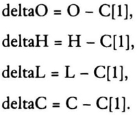
Here [1] denotes the close of the previous day. These equations encapsulate market trading behavior since they capture price patterns versus the previous close. Over a period of years, each market will have some characteristic values for these equations, based on its volatility, liquidity, and other trading patterns. When we sample with replacement using these formulas, we create patterns that bear the market’s signature as defined by relative price relationships.

The next step is to use a random number generator to scramble the bars. Once you have a new sequence, you need a starting point, usually the prior close. You can use any number for the first bar. The new bar is derived from the prior close as follows (new synthetic values are indicated by the Syn prefix):

So the calculations are easy to put into a program or a spreadsheet. We will first calculate the interbar relationships in Table 8.2, which is based on the actual bar sequence of the December 1995 S&P-500 (Figure 8.1). The interbar relationships appear in the last four columns. The difference between the daily close of 11/30 and 11/29 was –0.80 points. The differences between yesterday’s close and today’s open, high, low, and close are shown for each day. These calculations encapsulate price relationships. Now we can scramble these bars using a random number generator.

To scramble these data, number them from 1 to n, where n is the last bar. Then, use the random number generator to pick a number between 1 and n. That number is the next bar in the sequence. Suppose on the tenth pick, you pick bar 5. Then the original bar 5 becomes bar 10 of the new sequence. The bars may repeat more than once. For example, on the twenty-seventh pick, you may draw bar 5 once again. You can generate as long a sequence as you desire.

Here we used the 11/29/95 close of 608.05 as reference, and generated a new sequence of bars using the sampling function in Microsoft Excel®. The new sequence was: 4, 5, 8, 1, 3, 10, 10, 8, 9, 1. Therefore, starting with the previous close of 608.05, we put in the fourth bar of the original data, then the fifth bar, and the eighth bar, and so on.

Table 8.2 Spreadsheet based on December 1995 S&P-500 data.

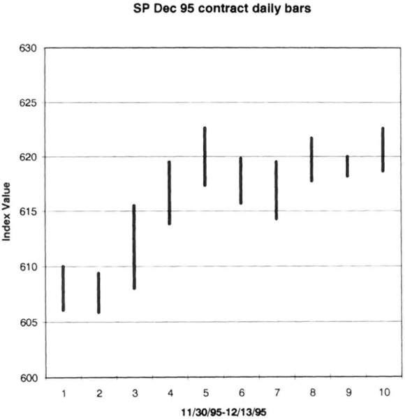
Figure 8.1 Actual price bars from the December 1995 S&P-500 contract.

Table 8.3 Scrambled data for S&P-500 using relationships calculated in Table 8.2. I assumed that the close before the first bar (bar 4 below) was 608.05.

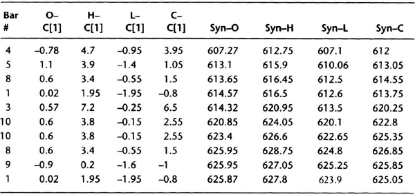
Table 8.3 presents the spreadsheet used to calculate the new synthetic data. The first column is the bar number drawn by sampling with replacement. The next four columns are the inter-bar relations previous calculated for each bar in Table 8.2. The last four columns are the synthetic data derived from the previous close by adding the interbar relations.

In Table 8.2, the data for 12/05 converts to bar 4, and the market gained 3.95 points on the close. In Table 8.3, bar 4 is the first bar of the new sequence. The previous close was assumed to be 608.05. So the new close is 3.95 + 608.05, or 612.00. The new low is 608.05 – 0.95, or 607.10. The new high is 4.7 + 608.05, or 612.75. These are the numbers for the synthetic contract in the first row. The close for the second bar is 612.00 + 1.05 or 613.05. You can now complete the rest of the calculations. The new scrambled data created a synthetic bar pattern plotted in Figure 8.2.

The new bar sequence (Figure 8.2) shows an upward bias, getting up toward the 630 area. Note how it does not show the consolidation in the last six bars of the original data. The last bar from the original data (bar 10 on Figure 8.1) occurs in Figure 8.2 as bars 6 and 7, and you can see that the relative appearance of the high and low versus the previous bar in the sequence is similar in both cases. Thus, we have encapsulated the market behavior in the original bar 10 and reproduced it in another sequence to create new synthetic data.

Of course, the more samples you generate, the greater the variety of patterns you will see. Another synthetic pattern derived from original December 1995 S&P-500 futures data is shown in Figure 8.3 to illustrate the variety of possible patterns. The new patterns cover a narrower price range than the original data, and appear like a breakout at the end.

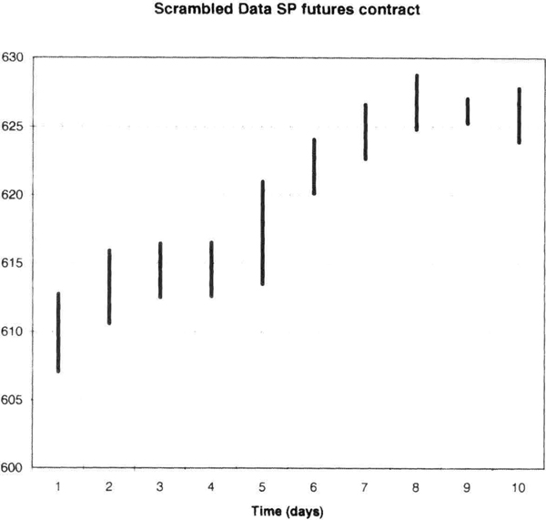
Figure 8.2 Synthetic data from Table 8.3 for the S&P-500 contract.

Thus, you can generate a variety of chart patterns using data scrambling. Continuous contracts work well to create synthetic data because they represent a long history of market action. If you prefer, you can use this method on individual contracts, and then string them together for testing using rollovers at the appropriate dates.

The power of data scrambling increases as the number of bars of data increases because you can create a greater variety of patterns. Thus, if you had, say, a 5-year or 7-year long continuous contract, you could generate 100 years of data and test your system against a variety of market conditions. Since these are the type of patterns you are likely to see in the future, this is the most rigorous out-of-sample testing you can achieve.

Figure 8.4 shows how data scrambling can overcome the limitation of insufficient data. First, the original data had several trading ranges, whereas the synthetic data has several trends, indicating you can generate new price patterns. Second, the synthetic data exceeded the price range of the original. Thus data scrambling can create new price ranges and new price patterns, which are necessary to test your system under the widest possible range of market activity.

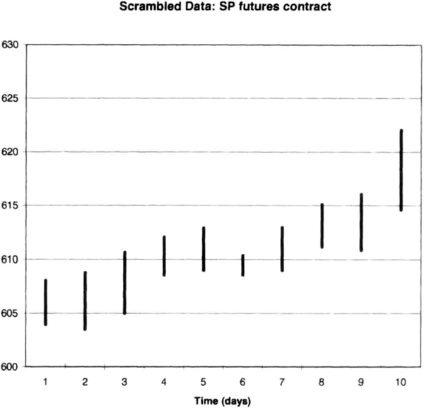
Figure 8.3 Synthetic data for S&P-500 contract using the bar sequence 6, 5, 4, 2, 1, 9, 10, 8, 7, 3.

Figure 8.4 Swiss franc synthetic contract (lower curve) generated from daily data using continuous contract (upper curve).

Testing a Volatility System on Synthetic Data

Here we test a volatility system on synthetic data to illustrate how to use data scrambling. A volatility system is a good choice for this because the currency markets have recently seen sudden, compressed moves. You may feel that sudden, compressed price moves are a staple in today’s futures markets. However, a historical review will convince you that they have also occurred before. Such moves are often difficult to trade with systems that use heavily smoothed data. Many traders have observed that sudden moves also occur near the turning points of trends. Hence, you may find a volatility-based approach also suitable for identifying tops or bottoms. You can define volatility in many different ways.

The usual practice is to use some multiple of the recent true range to define the edges of price moves. Here we take a simpler approach and use just the difference between today’s high and low as the measure of price range. The buy stop for tomorrow is today’s high plus two times today’s high-low range. Similarly, the sell stop is today’s low minus two times today’s high-low range. It is quite unlikely (but not impossible) that you will hit both entry orders on the same day.

The above definition of entry points is quite generic and not optimized to any specific market. You can use a multiple larger than two to get fewer entries, or smaller than two if you want more entries. We assume these volatile swings occur near turning points, so we will test an arbitrary trend following exit: exiting on the close of the twentieth day in the trade. First we look at test results using continuous contracts. Then, we will test this system on synthetic Swiss franc data obtained using data scrambling. The goal is to show how this simple system works as well as to illustrate how you can use scrambled data.

Figure 8.5 shows how the volatility entries appear on the December 1995 Swiss franc contract. In September, this system profited from a powerful rally. The exit at the end of 20 days got you out in the consolidation region. However, the system did not go short soon enough in the August sell-off. That trade was barely profitable. Note the previous long trade hit the $3,000 initial stop. Therefore, by design, a short burst out of one consolidation into another consolidation or trend works best with this system.

We tested the system first on a continuous contract using actual Swiss franc data from June 30, 1989, through June 30, 1995, allowing $100 for slippage and commissions and using a $3,000 initial stop. We then used the data scrambling routine to scramble these data, and made up eight more continuous contracts. We tested the same system without any changes on the scrambled data, as summarized in Table 8.4. The synthetic data have the letters “Syn” in their name for clear identification.

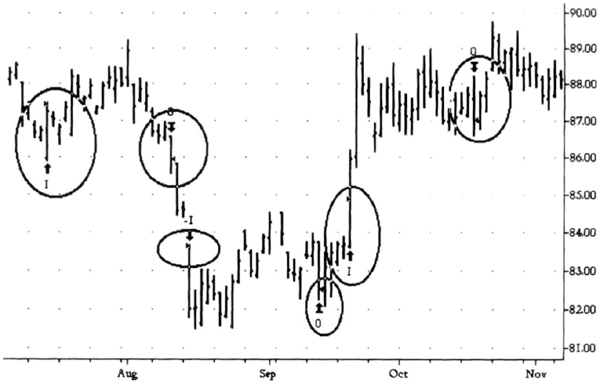
Figure 8.5 Stops at two times the high-low range above and below today’s high and low provide good entries into compressed moves. However, the market can often make big moves without volatility.

Table 8.4 Comparison of volatility system on actual and scrambled data.

The results over 56 years of synthetic data show that it is possible to have future performance significantly better or worse than the test period. This should come as no big surprise. The performance over individual synthetic contracts varies widely. The average performance of all the eight synthetic series (last row), however, approaches the performance over the original test period (first row). This result is similar to that shown in Table 8.1, where the average statistics of the random samples were close to the statistics of the original sample.

In essence, when we average the results over more and more synthetic data, we will get ever better estimates of the “true” or most likely system performance. We can also find the standard deviation of the results over synthetic data to quantify the variability of future results. For example, the standard deviation of the profits on synthetic data in Table 8.4 was $20,523 (not shown). Armed with this data, we can use mean-variance analysis to make portfolio decisions using the ideas of modern portfolio theory. We can try to find the portfolio weights for a group of systems that might achieve a given level of expected return for a particular expected standard deviation. We can also use the standard deviation to input a relevant range of values for risk of ruin calculations. Another application is to estimate a range of future drawdowns for a given system. Thus, synthetic data can be used to estimate the expected future performance.

There is one important limitation of scrambled data. Since we are using a random sampling with replacement approach, our new patterns do not represent actual market behavior. For example, synthetic data can create patterns that do not represent market psychology or any real supply-demand forces. Hence, you should create many data sets and average your system performance across those sets. The averaged performance will probably be more representative of potential system performance in the future.

Summary

In summary, scrambled data provide a new method to test a system over many different market conditions. You can observe the model’s performance under such simulations, and gain much needed confidence on how it works and learn to recognize when it does not. You can then use your insight to create filters that may improve system performance, reduce the number of trades, and create a neutral zone for system trading. You can also develop equity curves to check your interval estimates of standard deviation and therefore improve your projections of future drawdowns. You can also perform a subjective evaluation of market conditions under which the system does particularly well or poorly.