Chapter

Developing and Implementing Trading Systems

Introduction

Trading has been called the hardest way to make an easy dollar. To be consistently profitable, we must all climb the trader’s mountain (see Figure 1.1). Top traders are internal attributors who take personal responsibility for their trading success. The foundation of their success is adequate capitalization coupled with an unwavering commitment to excel at trading. Successful traders have sufficient trading capital to withstand losing periods, as well as to trade many markets with multiple contracts. These traders simply love what they do, are constantly searching for better trading concepts, and devote the time and energy necessary to achieve their trading goals.

Capital conservation is just as important to top traders as capital appreciation. They know better than anyone the importance of having trading capital when the markets finally move in their favor. Top traders use sound money-management principles and rigid risk control to preserve capital during difficult market conditions.

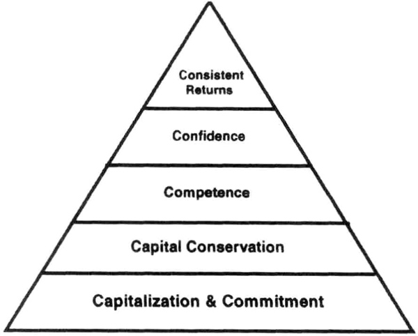
Figure 1.1 The mountain a trader must climb for trading success.

All successful traders have developed specific trading competencies that match their style and objectives. They understand their trading preferences, and have developed the analytical tools and execution capabilities that allow their trading process to be implemented smoothly and, it seems, effortlessly. They have the patience and persistence to stick with a trading strategy and to review it periodically for upgrades and improvements. In essence, they test what they trade and trade what they test.

Winning traders are supremely confident about their abilities to be profitable over the long run. They are not surprised by losing periods, and they retain an optimistic and positive attitude under the most trying conditions. Their capitalization, money management, risk-control procedures, and competencies further help them keep the faith. Their confidence makes them disciplined and systematic in everything they do. This book will help you to develop the competencies needed for consistent performance, teach you the latest ideas on controlling risk, and give you the confidence to systematically trade what you test. Trading is analysis in action, and this book will empower you to go beyond technical analysis.

What’s New in This Edition

This book can be divided into parts. The first part of the book, comprising the first five chapters, shows you how to build robust trading systems consistent with your beliefs. The second part, comprising the remaining chapters, discusses money management, risk control, and the implementation of trading systems. This second edition preserves the structure of the first edition and strengthens it by adding new material, derived primarily from personal research, that emphasizes capital preservation, robust system testing, and trading psychology. In response to reader comments, Chapters 1 and 3 contain new review material to help you to survey the basic principles of technical analysis, avoid common pitfalls in system testing, and assess the strategic design tradeoffs in selecting entries and exits. Chapter 4 of this edition updates the performance of the key systems discussed in the first edition by testing these systems on a global portfolio with multiple contracts, to see how they would have fared in a true “out-of-sample” test on a million-dollar account. Next, we demonstrate that all the ideas in this book can be applied to stock trading by testing a new system on stocks and futures.

The bulk of the new material is concentrated in Chapters 6 and 7. Chapter 6, Equity Curve Analysis, now explains how to account for commodity trading advisor (CTA) performance by modeling CTA returns. It then discusses how to develop stabilized money manager rankings, so you can develop portfolios that are more efficient. A detailed discussion of risk-adjusted performance measures and an actual comparison of different measures allow you to choose the one you like best. Chapter 6 ends by developing a control chart of future performance so you can monitor CTA performance more effectively.

Chapter 7 features new material on estimating the three key unknowns of future performance: depth of drawdowns, duration of drawdowns, and expected returns. It builds quantitative models to estimate these key measures for a diversified portfolio of futures, hedge funds, or stocks. The application of these ideas is shown via the Chande Comfort Zone, an essential tool for systematic trading. This chapter shows how you can use these models to deal with drawdowns, and answers the crucial question: has the system stopped working? Additional models for scaling volatility, scaling leverage, and establishing benchmarks for calibrating risk-adjusted returns are included. Chapter 7 discusses empty diversification and shows an example comparing CTAs. The chapter ends by applying these ideas to the trading of stocks and mutual funds. The ideas in this book advance the state-of-the art in risk control and money management by providing portfolio-level solutions.

Chapter 9 shows how you can build an automated diary using a spreadsheet. The last of the new material in Chapter 9 applies sports psychology in trading. Trading exerts enormous pressures on traders, as does the field of sports on its professionals. Hence, it is natural to ask how the techniques of dealing with the mental demands of sports can be applied to trading. Chapter 9 shows how the basic ideas taken from sports can be adapted to the trading environment, to help traders deal with the stresses of trading. As with other issues in psychology, this is but one interpretation, and you may wish to apply these ideas differently. However, the ideas may provide a useful starting point for your own research into this important aspect of trading.

The Usual Disclaimer

Throughout the book, a number of trading systems are explored as examples of the art of designing and testing trading systems. This is not a recommendation that you trade these systems. I do not claim that these systems will be profitable in the future, nor that profits or losses will be similar to those shown in the calculations. In fact, there is no guarantee that these calculations are defect free. I urge you to review the section in Chapter 3 called a reality check. That section points out the inherent limitations of developing systems with the benefit of hindsight. You should use the examples in this book as an inspiration to develop your own trading systems. Do not forget that there is risk of loss in futures trading.

What Is a Trading System?

A trading system is a set of rules that defines conditions required to initiate and exit a trade. Usually, most trading systems have many parts, such as entry, exit, risk control, and money management rules.

The rules of a trading system can be implicit or explicit, simple or complex. A system can be as simple as “buy sweaters in summer,” or “buy when she sells.” By definition, the system must be feasible. Ideally, the system accounts for “all” trading issues, from signal generation, to order placement, to risk control. A good way to visualize effective system design is to stipulate that someone who is not a trader must be able to implement the system.

In practice, every trader uses a system. For most traders, a system could really be many systems. It could be discretionary, partly discretionary, or fully mechanical. The systems could use different types of data, such as 5-minute bars or weekly data. The systems may be neither consistent nor easy to test; the rules could have many exceptions. A system could have many variables and parameters. You can trade different combinations of parameters on the same market. You can trade different parameter sets on different markets. You can even trade the same parameter set on all markets.

What Is a Trading Program?

Clearly, no universal trading program exists, although the components of a successful trading program for stocks or futures can be easily identified (Table 1.1). The process of signal generation requires the trader to analyze data sources, determine the portfolio of markets or stocks to be traded, and feed that information continuously into the signal generator. The generated signals must then be correctly sized for the account equity, and the trade sizing algorithm must also include money management considerations. The output of this effort is a valid buy or sell order. The trader can then send the orders to a broker for execution. The trader must carefully monitor execution, check for fills and errors on the desks, and follow up by checks on the daily and monthly statements. Successful traders prepare for market holidays and their own vacations. They also have backup and redundant systems to allow for interruptions of data feeds, electrical power, and communication links. The last set of challenges, checks and balances, requires the trader to develop procedures for handling trading errors and overall risk controls. The trader must also monitor his or her own psychological condition and maintain a vigorous research program.

Table 1.1 Components of a successful trading program.

Every trader adapts a “system” to his or her style of trading. It would be helpful to classify trading systems into different types of return generation processes (RGPs) for ease of analysis and comparison. You will also find it easier to visualize your own trading style by understanding the classification scheme for RGPs proposed in the next section.

Classification of Return Generation Processes

A return generation process is simply a trading system or portfolio of systems. A simple and consistent system classification by style would facilitate a comparison of different RGPs. Such a method of classification should be useful for investors and allocators alike in their search for superior performers.

The RGP is the trading “system” by which equity is risked in order to seek profits. The variable that differentiates RGPs is the time frame over which prices are expected to move in favor of a given position. The time frame is quantified as the length of the average winning trade in trading, not calendar, days. On average, the longer the trade duration, the larger the amplitude of the expected move, and the larger the average profit per trade. A “slow” trading system tends to have trades of longer duration. Hence, the average duration of winning trades is a valid parameter for classifying RGPs.

We begin by separating the RGP into entry and exit strategies. Each RGP needs at least one of each, but may have one or more of both. We then classify the “speed” of trading into two levels, fast and slow. The speed labels describe the relative sensitivity of the entry and exit signals to price action. Faster entries and exits tend to be more sensitive to price movements. Because there are two levels each for the entry and exit, there are a total of four style combinations (Figure 1.2). The values of average trade duration assigned to the four style categories shown in Figure 1.2 are based on personal experience.

Figure 1.2 A classification of return generation processes by duration of winning trades.

We can now convert the average trade duration into distinct RGP styles (Figure 1.3). Brute-force trend-following is an RGP that generally uses slow entry and exit strategies. Average trade lengths are typically greater than 50 days, and such RGPs are robust and have stood the test of time. These RGPs come in a variety of flavors, take moderate risks for large profits, and work best with large accounts using a diversified portfolio. They are susceptible to drawdowns when a large portion of open trade equity is lost due to slow exit strategies.

The diagonal opposite of brute-force trend-following is “hot-button” trading, which lasts less than 5 days. These high-speed RGPs use fast entries and fast exits, trade a relatively small number of markets, must control slippage and execution costs, and work best when there are “burst” moves lasting three or more days. They are susceptible to choppy price action, often take large risks for small profits, and are vulnerable to correlation shifts and pattern failures. Hot-button RGPs tend to have a low correlation to other RGPs, and are usually traded with small accounts or vast leverage.

An RGP that gets into an emerging trend early and stays until the trend is exhausted can be called an “early-bird special.” This works best when markets trend smoothly in a given direction (like migrating birds), but is susceptible to false breakouts or early trend reversals. Hence, this strategy can also be viewed as optimistic trend-following. Such RGPs are also robust, but tend to give up some equity before closing successful trades. An antitrend strategy may be visualized as belonging to this category.

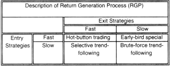
Figure 1.3 Descriptive classification of RGPs.

The last remaining RGP style can be called selective trend-following because it seeks well-established trends. Because such RGPs are slow to enter and quick to exit, they are less vulnerable to early reversals or late setbacks during trends. However, the price of such RGPs is lost market opportunities when trends are smooth and orderly, even though they have excellent risk adjusted performance.

Figures 1.2 and 1.3 can help you to classify your own style or that of a trading advisor. If the advisor uses a blend of strategies, then a weighted average trade duration can be used to classify that manager. The investor or allocator can now create portfolios with a blend of these RGPs, or a preponderance of these RGPs, in order to meet their investment goals. For example, a portfolio may include a brute-force trend-follower and a selective trend-follower to add extra returns when trends are strong while reducing down-side volatility when trends are particularly scarce.

The strengths and weaknesses of each style are summarized in Table 1.2. An investor or allocator can use this generalized classification scheme to understand or test the strengths and weaknesses of any particular RGP. It is easier to sort through conflicting claims by identifying the style of a manager because performance should be generally similar within a style classification. You can also use your own data to have three speed categories, fast, medium, and slow. In conclusion, you can use this approach to construct effective portfolios. Yet another approach to classifying RGPs is discretionary versus fully systematic, as discussed in the next section.

Table 1.2 Comparison of RGP strengths and weaknesses.

Comparison: Discretionary versus Mechanical System Trader

Table 1.3 compares two extremes in trading: a discretionary trader and a 100 percent mechanical system trader. Discretionary traders use all inputs that seem relevant to the trade: fundamental data, technical analysis, news, trade press, phases of the moon—their imagination is the limit. System traders, on the other hand, slavishly follow a mechanical system without any deviations. Their entire focus is on implementing the system “as is,” with no variations, exceptions, modifications, or adaptations of any kind.

Exceptional traders are discretionary traders, and they can probably outperform all mechanical system traders. Their biggest advantage is that they can change the key variable driving each trade, and therefore vary bet size more intelligently than in a mechanical system. Discretionary traders can change the relative importance of their trading variables so they can easily switch between trend-following and anti-trend modes. They can instantly switch between time frames of analysis, going from 5-minute bars to weekly bars as their assessment of the trading opportunity changes.

Discretionary traders can make better use of market information other than price. For example, they can react to news or fundamental information to change bet size. Discretionary traders can adjust their perceived risk constantly, so they can increase or decrease positions more intelligently than mechanical traders. These infrequent “home runs” often make all the difference between good and great trading performance. However, for the average trader, being a mechanical system trader probably maximizes the chances of success.

The goals of a mechanical system trader are to pick a time frame (for example, hourly, daily, weekly), identify the trend status, and anticipate the direction of the future trend. The system trader must then trade the anticipated trend, control losses, and take profits. The rules must be specific, and cover every aspect of trading. For example, the rules must specify how to calculate the number of contracts to trade and what type of entry order to use. The rules must indicate where to place the initial money management stop. The trader must execute the system “automatically,” without any ambiguity about the implementation.

Table 1.3 Comparison of the information-based style of a discretionary trader to the data-driven style of the fully systematic trader.

Discretionary Trader	100% Mechanical System Trader
Trades “information” flow	Trades “data” flow
Anticipatory traders	Participatory traders
Subjective	Objective
Many rules	Few rules
Emotional	Unemotional
Varies “key” indicator from trade to trade	“Key” indicators are always the same
Few markets	Many markets

Mechanical system traders are objective, use relatively few rules, and must remain unemotional as they take their losses or profits. The most prominent feature of a mechanical system is that its rules are constant. The system always calculates its key variables in the same way regardless of market action. Even though some indicators vary their effective length based on volatility, all the rules of the system are fixed, and known a priori. Thus, mechanical system traders have no opportunity to vary the rules based on background events, nor to adjust position size to match the markets more effectively. This is at once a strength and a weakness. A major benefit for system traders is that they can trade many more markets than can discretionary traders, and achieve a level of diversification that may not otherwise be possible.

You can create different flavors of trading systems that use a small or limited amount of discretion. You could, for example, have specific criteria to increase position size. This could include fundamental and technical information. You can be consistent only if you are specific. This discussion really begs the question of why to use trading systems, answered in the next section.

Why Should You Use a Trading System?

The most important reason to use a trading system is to gain a “statistical edge.” This often-used term simply means that you have tested the system, and the profit of the average trade—including all losing and winning trades—is a positive number. This average trade profit is large enough to make this system worth trading—it covers trading costs, slippage, and is, on average, likely to perform better than competing systems. Later in the book, I discuss all of these criteria in greater detail.

The statistical edge is relevant to another statistical quantity called the probability of ruin. The smaller this number, the more likely you are, on paper, to survive and prosper. For example, if you have a probability of ruin less than, say, 1 percent, your risk control measures and other measures of system performance are typically sufficient to prevent instant destruction of your account equity.

My biggest source of concern about these statistical numbers is they assume you will trade the system exactly as you have tested it, with not one deviation. This is difficult to achieve in practice. Thus, your risk of ruin—and it is only a risk until it becomes a fact—could be higher than your calculations. Despite this concern, you should develop systems that meet sound statistical criteria, for that greatly enhances your odds of success. As usual, there are no guarantees, but at least the odds, if not the gods, will be on your side.

Another reason to use a trading system is to gain objectivity. If you are steadfastly objective, you can resist the siren call of news events, hot tips, gossip, or boredom. Suppose you are a chart trader and you enjoy some flexibility in interpreting a given chart formation. It is very easy to identify a pattern after the fact, but it is rather difficult to do so as the pattern evolves in real time. Hence, analysis can paralyze you, and you may never make an executable trading decision. Being objective frees you to follow the dictates of your analysis.

Consistency is another vital reason to use a trading system. Since the few rules in a trading system are applied in precisely the same way each time, you are assured of a rare consistency in your trading. In many ways, objectivity and consistency go together. Although consistency is known as the hobgoblin of little minds, it is certainly a useful trait when you are not quite a champion trader.

A trading system gives another crucial advantage: diversification, particularly across trading models, markets, and time frames. No one can be certain when the markets will have their big move, and diversification is another way to increase your odds of being in the right place at the right time.

In summary, you can use a trading system to gain a statistical edge, objectivity, consistency, and diversification across models and markets. A key assumption underlying this section is that the system you are using is well designed and robust. The next section discusses examples of a robust trading system.

Robust Trading Systems: TOPS COLA

A robust trading system is one that can withstand a variety of market conditions across many markets and time frames. A robust system is not overly sensitive to the actual values of the parameters it uses. It is not likely to be the worst or best performer, when traded over a “long” time (perhaps 2 years or more). Such a system is usually a trend-following system, which cuts losses immediately and lets profits run. This philosophy, called TOPS COLA, merely says “take our profits slowly” and “cut off losses at once.”

Two examples of robust systems are a moving-average cross-over system and a price-range breakout system. Both systems are well known, and are widely traded in some form or another. The trades from these systems typically last more than 20 days. Hence I classify them as intermediate-term systems. They are trend-following in nature, in that they make money in trending markets and lose money in nontrending markets. The typical system has a winning record of 35 to 45 percent, with an average trade of more than $200. I will discuss these systems in detail later.

The key feature to note is that, when systematically implemented over a “long” time and over many markets, robust systems tend to be, on the whole, profitable. If executed correctly, they guarantee entry in the direction of the intermediate trend, cut off losses quickly, and let profits run. Countless variations of these systems exist, and trend-following systems seem to account for a large percentage of professionally managed accounts.

Robust systems do not make many assumptions about market behavior, have relatively few variables or parameters, and do not change their parameters in response to market action. There is no sharp drop in performance due to small changes in the values of system variables. Such systems are worthy of consideration in most portfolios, and are reasonably reliable. In addition, they are easy to implement.

What Is a “Good” Trading Program?

You can use the tools in this book to develop “good” mechanical systems; that is, systems you can trade systematically, without any deviations, and without worrying about each position every day. Systems must be combined with risk control guidelines and money-management algorithms to construct trading programs. But how do you know you have a good program? Table 1.4 presents a simple checklist that you can use as a guide or benchmark. Remember, there are no guarantees; however, the following suggestions should put you on the right track and are typical of the long-term performance of professional money managers. You can expect to see considerable variation, depending on the time period used for the comparison. For example, the return efficiency can range from 0.1 to 0.5, with mutual funds in the 0.35 to 0.40 area, given the recent strong market performance. The expected drawdown is about four to five times the standard deviation of monthly returns; hence, it makes little sense to trade a program with monthly standard deviations greater than 15 percent. These guidelines assume that you are trading daily data, selecting systems using risk-adjusted performance (via return efficiency) and willing to tolerate drawdowns equal to four times the standard deviation of monthly returns. The goal of any parameter choices is to maximize the number of trades over the test period with an eye toward robustness.

Table 1.4 A proposed benchmark for a “good” mechanical trading program consistent with your trading beliefs.

Description	Units
Total Entry Conditions/Parameters	≤ 10 #
Total Exit Conditions/Parameters	≤ 10 #
Number of markets traded	≥ 10 #
Test period/data	≥ 24 Months
Equity risked per trade	≤ 2 %
Proportion of profitable trades	≤ 50 %
Average monthly return (μ)	1 %
Standard deviation of monthly returns (σ)	5 %
Return Efficiency (μ/σ)	≥ 0.2 #
Expected depth of drawdown	20 %
Expected duration of drawdown	≤ 9 Months
Proportion of profitable months	≤ 65 %
Expected Return	> 13 %

These guidelines are probably a good indicator of when you can stop your “search for the Holy Grail” and start trading the program. With sufficient work and originality, you can probably develop a program that can beat these guidelines. However, it is not enough to design a good program—you must also be able to implement it seamlessly.

How Do You Implement a Trading System?

Begin with a trading system you trust. After sufficient testing, you can determine the risk control strategy necessary for that system. The risk control strategy specifies the number of contracts per signal and the initial dollar amount of the risk per contract. The risk control strategy may also specify how the initial stop changes after prices move favorably for many days.

The system must clarify portfolio issues such as the number and type of markets suitable for this account. The trading system must also specify when and how to put on initial positions in markets in which it has signaled a trade before commencement of trading for a particular account.

A trade plan is at the heart of system implementation. The trade plan specifies entry, exit, and risk control rules along with the statistical edge. You should record a diary of your feelings and the quality of your implementation, plus any deviations from the plan and the reasons for those deviations. You should monitor position risk and the status of all exit rules.

Last, take the long view: Imagine you are going to implement 100 trades with this plan, not just one. Thus, you can ignore the performance of any one trade, whether profitable or not, and focus on executing the trade plan. These and other implementation issues are discussed in detail in Chapter 9.

Is Systematic Trading Easy?

Systematic trading is not easy because it is against human nature. Trading is an emotional endeavor, and systematic trading requires the trader to execute a set strategy for a “long” time without deviations (i.e., without emotions). This makes trading a boring activity, and thus counter to human nature. It takes a lot of patience and discipline to stick with your plan when the markets are going against your strategy. The markets are constantly presenting traders with information to challenge their trading beliefs, encouraging deviations from the predefined plan. For example, if you are an antitrend trader, the market will present you with a series of trends that go through your risk control stops instead of reversing as expected. Or, if you are a breakout-style trader, the market will confront you with a sequence of false breakouts that tempt you into an antitrend strategy.

Figure 1.4 Typical reactions of traders to the stresses of trading.

You need very strong beliefs in your trading process to stay with it without constantly tampering with the parameters (Figure 1.4). For example, the trader who truly believes in the system is prepared for drawdowns when they arrive, and can patiently grind out the worst periods, perhaps deleveraging the system if necessary. A trader with only moderate confidence goes from a state of tensely monitoring performance to increasing skepticism, and then a strong desire to modify or optimize the system. The trader with weak beliefs often starts out with excessive confidence in the system, which evaporates rapidly, so that he or she begins to ignore trading signals; this trader is late to get in and quick to get out. This trader abandons all hope as well as the system itself, and begins the destructive cycle anew with another system he or she barely believes in.

How, then, can you build confidence in a system? It begins with a knowledge of your trading beliefs, a topic covered in detail in Chapter 2. Then, you must have confidence in your testing. All the material in this book is designed to give you that confidence. Next, you must have realistic expectations. Guidelines for a “good” program as well as a discussion of return-efficiency benchmarks appear in Chapter 7. Last, you must trade what you test; Chapter 8 and the discussion on sports psychology in Chapter 9 will help.

Trading is often an error-prone process, and the market quickly discovers your weakest links. The market will repeatedly create conditions to test your weaknesses. For example, if you have problems with the data feed, those problems will occur at the most inopportune times. If you need to leave the office early on Tuesdays, these crises will occur on Tuesdays, as if by magic. Thus, the entire trading process must be constantly examined and maintained at the highest state of readiness, an unexciting but necessary chore.

Another problem with trading is that the returns are variable, and it can be difficult to keep your balance whether you are winning or losing. During testing, vast amounts of data are crunched in milliseconds. In real time, however, you cannot accelerate the clock, and you must live through every drawdown one day at a time. Thus, the variability of returns can also work against your desire to stick with a trading strategy.

Is anyone really systematic? A surprisingly large number of the professionals are. For example, money managers are systematic. Index fund managers are systematic. Even casinos are systematic; they understand they have a small edge, and the more bets people place, the more likely it is that the “house” will be profitable. Insurance companies understand that the more people they insure, the less the risk to the entire portfolio. Thus, systematic trading can be profitable over the long run, if you understand that you have to live through the difficult times to be around when the market conditions favor your strategy. Systematic trading is difficult to execute over a long time, but if you master the psychological challenges, you will clearly have an edge. If you do not wish to be systematic, then find out who wins and who loses in the next section of this chapter.

Who Wins? Who Loses?

Tewles, Harlow, and Stone (1974) report a study by Blair Stewart of the complete trading accounts of 8,922 customers in the 1930s. That may seem like a long time ago, but the human psychology of fear, hope, and greed has changed little in the last 70 or so years. The results of the study are worth considering seriously.

Stewart reported three mistakes made by these customers: (1) Speculators showed a clear tendency to cut profits short, while letting their losses run; (2) Speculators were more likely to be long than short, even though prices generally declined during the nine years of the study; and (3) Longs bought on weakness and shorts sold on strength, indicating they were price-level rather than price-movement traders.

I should contrast this experience with the TOPS COLA philosophy discussed earlier. By taking profits slowly and cutting off losers at once, you will avoid the first mistake reported by Stewart. Second, by being a trend follower, you will avoid the next two mistakes. If you follow trends, you will be long or short per the intermediate trend, and avoid any tendency to be generally long. Third, if you follow trends, you will follow price movement, rather than being a price-level trader.

You will win in the trading business if you have a specific trade plan that contains all the necessary details. You should focus much of your effort and energy on implementing the trade plan as accurately and consistently as possible. Thus, you must go beyond technical analysis, deep into trade management and organized trading, to win.

Appendix to Chapter 1: A Brief Technical Analysis Primer

Introduction

This primer is intended for anyone unfamiliar with the fundamental ideas of technical analysis. If you are familiar with the basic ideas of technical analysis and can use commercial technical analysis software programs, then you can skip this appendix entirely. However, it does include the code for adaptive oscillators and adaptive moving averages that some of you advanced readers might find useful.

There are two types of market data: external and internal. External data are generated by economic activity, regulators, or governments—factors influencing supply and demand, production, and consumption. External data are called fundamental data. Internal market data are generated by the process of trading an instrument such as stocks, futures, or options, and are collected and disseminated by the trading exchanges. Trading data are called technical data. Hence, technical analysis is the analysis of internally generated market data. There are different kinds of internal data, depending on how and where an instrument is traded.

Trading a stock or futures contract generates such information as the price at which the instrument was traded, the number of contracts or units traded, and whether a new position was opened or an existing position was closed. When all the trades in a day are collected and summarized, the exchanges report the daily trading range (high and low), the opening price, the closing price, the trading volume, and the open interest. If you do not understand what each of these terms means, you can visit the Web sites of any futures or stock exchange.

Technical market data are analyzed by plotting them on a graph or chart, in which the horizontal axis is time and the vertical axis describes the units of technical data. The horizontal (time) axis of the graph may depict yearly, monthly, weekly, daily, or intraday periods. The vertical axis shows the price activity: the opening, high, low, and closing prices in local currency. For stocks in particular, the volume of activity during the period is plotted immediately beneath the price bar. Because the price range looks like a bar, this is usually called a bar chart.

Over time, creative traders have observed, invented, tested, and cataloged hundreds of ideas about analyzing bar charts. The advent of computers has simplified this analysis, while permitting other more computationally intensive analytical approaches. It is impossible to describe the myriad ideas in a few short paragraphs, but some important elements that are relevant to understanding the material presented in this book are summarized here.

Assumptions of Technical Analysis

Perhaps the most important assumption of technical analysis is that history repeats itself, and past price action has important implications for future price action. The second major assumption is that a trend in force continues in that direction until replaced, and the trend in a longer time frame (say monthly) is more important than a trend in a shorter time span (say daily). The third assumption is that all currently available information in the public domain about the instrument being traded is fully reflected in the market. This implies that no trader has an information edge, which is not necessarily true. You can debate the validity of these assumptions, and a number of academic studies are available that raise questions about them, insider trading and the random walk theory being two obvious examples. However, for all practical purposes, we will take these assumptions to be generally correct.

Technical analysis relies on detecting patterns in the past that can be traded with confidence in the future. The identification and quantification of patterns can be subjective or objective. Subjective patterns include various types of price formations on a chart, such as channels or triangles. Objective measures of prices are algorithmic formulations, such as moving averages and oscillators. Here we focus on the quantitative elements of technical analysis and refer you to other books on technical analysis for a discussion of chart patterns.

Typical Price Patterns and Chart Formations

Some common price patterns and chart formations using data from the futures markets are shown in Figures 1.5 through 1.13. The same terms are used with stock charts.

A trending market shows prices that move steadily in one direction, either up or down (Figure 1.5). These trends can be traded by taking a position in the direction of the trend. Trends occur in response to fundamental developments that attract buyers willing to pay ever-higher prices or draw out sellers willing to sell at ever-lower prices. In the language of economics, the equilibrium price is far away from the current price, and prices move toward the perceived future equilibrium price. Trends can cover a very wide range in prices, with stocks covering a much larger range in prices than futures.

Figure 1.5 A continuous contract of the Eurex Swiss Federal Bond illustrating basic chart patterns.

A trading range usually occurs at the end of trends, when the prices are close to the perceived equilibrium price and “move sideways” or are contained within some range of values (see Figure 1.5). The usual interpretation here is that the market finds supply at the high end of the trading range (more aggressive sellers) and support at the lower end of the range (more aggressive buyers). One cannot say that there are more buyers than sellers because each trade must match buyers and sellers. Note that there can be an increase in the open interest or in the short interest for stocks if there is a preponderance of sellers or buyers. Such markets are best traded with an antitrend approach that buys lows and sells highs. A trend-following approach using moving averages will be unprofitable because prices move back and forth, producing a succession of losing signals in both directions.

A choppy market lacks conviction about price direction, with drifts in one direction and rapid moves in the other direction (see Figure 1.5). A choppy market may be viewed as a market trading within an expanded trading range. A choppy region could occur within a broad uptrend or downtrend, and could last from 1 to 5 months. Trend-following strategies using moving averages and breakout-style strategies are prone to losses within choppy markets. The markets generally break out of such ranges, but it is difficult to single out false breakouts with accuracy.

Figure 1.6 A continuous contract of the New York High Grade Copper showing swing moves in 1999.

A market is making swing moves (see Figure 1.6) when it moves smoothly from one price level to another within a very wide trading range over a 7 to 20 day interval. Trend-following strategies using moving averages will be more profitable than breakout-style strategies, and antitrend strategies will be unprofitable in such a market. Periods of swing moves may be viewed as extended consolidations and are usually followed by a trading range or choppy trading. Although such regions can be easily detected (after the fact) by the human eye, they are difficult to detect in real time using quantitative measures.

Cyclic markets make swing moves lasting 3 to 7 days covering a narrow trading range (Figure 1.7). They can be detected using computer-intensive methods and traded by anticipating turning points. Such conditions occur somewhat less frequently than is popularly believed.

Price channels form when swing moves or cyclic markets are superimposed on strong trends. When detected, they are easy to trade using simple trend-following tools. The London International Petroleum Exchange (IPE) Brent Crude futures contract showed a particularly neat channel during its uptrend in 1999-2000 (Figure 1.8). The initial rise in early 1999 was sufficient to define the channel that carried well into 2000. Discretionary traders would have enjoyed low-risk buying opportunities near the bottom of the channel with little follow through below the channel. The same discretionary traders were offered low-risk shorting opportunities near the top of the channel. Such powerful channels are rare, but do occur in both stocks and futures. They are found more frequently in stocks than futures.

Figure 1.7 A continuous contract of the Stockholm Options Market OMX Index showing strong cyclic pattern in 2000.

Figure 1.8 The London IPE Brent Crude futures continuous contract showing a well-defined price channel in the 1999–2000 period.

Figure 1.9 A continuous chart of the Chicago IMM Japanese Yen futures contract showing massive triangular consolidation in 1995.

Triangles represent a period of consolidation, when the market’s trading range contracts rapidly over time, forming a pattern that can be contained within a triangular shape. At least three types of triangles can be identified: symmetrical (Figure 1.9), ascending, or descending. In real time, the triangle defines the time period within which the market usually resolves the uncertainty about the future direction of prices (i.e., prices move decisively out of a triangle before the pattern is completed). These can be traded successfully by awaiting the price breakout. This pattern is also useful in option trading because volatility is likely to decrease when the prices consolidate within the pattern; volatility will probably increase when the prices break out of the pattern.

A double bottom or double top accurately describes the pattern in which prices make an initial extreme (low or high, respectively), then “retest” that extreme a second time, usually within a period of 1 to 4 months, and finally move decisively away from that extreme in the opposite direction. The retest can take many forms. When the prices come close to the previous extreme without going beyond that price, the pattern qualifies as a double bottom or double top. Occasionally the retest may result in the previous extreme price being exceeded by a small amount, without a close beyond the prior extreme. These patterns represent a loss of momentum, and are easy to detect by eye, but somewhat more difficult to define programmatically because the time between retests can vary widely.

Figure 1.10 A double bottom in a continuous contract of Italy’s Milan 30-Stock Index Futures (MIF) in late 1999.

Compare, for example, the double bottom formed over a typical period of 1 to 4 months in the Milan 30-Stock Index Futures (MIF) (Figure 1.10) to the massive double bottom that took about 10 months to form in the New York CSCE Sugar #11 futures contract (Figure 1.11). The definition of a double bottom embodies considerable subjectivity. However, as both charts indicate, it can be traded successfully. The aggressive trader may try to enter as close to the double bottom as possible in anticipation of the pattern. A more conservative approach is to buy above the high formed between the test of the low prices on either side of the double bottom. In the conservative approach, the early entrants are typically selling out to the late buyers, and a retest of the double bottom or a minor consolidation can occur here. A close above the high between the double bottoms is said to confirm the double bottom.

Measured Objectives from Chart Formations

Empirical observations have resulted in a consensus about the amplitude of future moves when prices show certain definable chart formations. Such amplitude projections are called measured objectives. In any given occurrence, the market may or may not achieve the expected amplitude, or may easily go on to significantly exceed the projected amplitude. However, the ability to recognize and categorize the pattern and make a projection about future price objectives permits the creation of a trading strategy around such patterns. The two examples shown here illustrate this idea, but are by no means a complete or exhaustive catalog of such patterns.

Figure 1.11 A massive double bottom in a continuous contract of the New York CSCE Sugar #11 futures that led to a powerful rally in 2000.

One often finds a rectangular price pattern on price charts, in which the prices have been trading in a “rectangle” for 4 to 6 months. The height of the rectangle can be used to derive a target for prices when they break outside the rectangle. Figure 1.12 shows a continuous chart for New York Cotton futures, with a rectangular price consolidation that occurred in the first half of 1999. The height of the rectangle was $7.25, and the projected downside target was 61.11. Once prices broke out of the consolidation, they reached the price target in less than a month.

Another well-known consolidation price pattern is the head-and-shoulder pattern, in which prices form an initial high, then the actual high, followed by a weak retest of that high. The retest fails at a lower level than the high for the move, forming the right shoulder. A trend line can be drawn under the lows of the pattern to form the “neck line.” Ideally, the neck line should be horizontal on the chart, but inclined neck lines are not unusual. This pattern can also be occasionally seen at market bottoms. The expected outcome after the formation of the pattern is a powerful move below the neck line for tops and above the neck line for bottoms. The head-and-shoulders pattern should be traded with caution because it has a relatively high failure rate. However, it does provide a means to derive a price target, measured from the highest high (or lowest low) to the neck line.

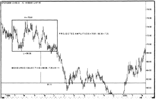
Figure 1.12 The measured objective is derived from a price rectangle as the height of the rectangle in this price chart of New York Cotton futures market.

Figure 1.13 shows a head-and-shoulders pattern in the London LIFFE Long Gilt futures continuous contract. The highest high on the continuous chart was 125.15, and the neckline intersects a vertical line from the highest high bar at 118.15, indicating a projected price target a full 7 points below the intersection price at 111.15. The Long Gilt broke below the neckline in May 1999, followed by a retest of the neck line seven days later. Once the retest failed, the Long Gilt traded lower in a choppy downtrend and reached the downside target 4 months later. Observe that the price target can be easily exceeded, as was the case with the Long Gilt in Figure 1.13.

Many classical books on technical analysis of stocks that describe measured objectives for patterns such as triangles, pennants, waves, and so on are available for further research in this area. You can probably derive many measurements on your own. You can use these targets as potential entry points or exit points in your systems, as long as you remember that the market will do what it wants.

Statistical Review

The arithmetic average, or mean, of a set of numbers is a summary statistic that summarizes some chosen property of the sample. The arithmetic average sums the chosen parameter over every item in the sample, and then divides that total by the number of items in the sample. For example, to find the average weekly closing price, add the daily closing prices from Monday through Friday, and then divide that sum by 5 to get the average weekly closing price. The average may be viewed as a weighted sum over all data points:

Figure 1.13 A downside target derived for the London LIFFE Long Gilt futures contract using a head-and-shoulder pattern for measurement.

where the weight w_i = (1/n), n = total number of data points, and V_i is the value of each data point. Hence, the average is an equally weighted sum of all the values in the sample, where the weight for each data point is simply the inverse of the total number of data points.

The average, or mean, of a sample does not give us any idea of how the data are scattered (or dispersed) about the mean; that is, we do not know how close to or how far away from the mean we will find data points. For example, calculating the average height of all the children in a class does not tell us either the range (the tallest minus the shortest) or the frequency of occurrence of different heights. We quantify the spread or dispersion in the data by the standard deviation.

To calculate the standard deviation, we first calculate the deviation of each data point from the mean (V_i – μ). The deviations are squared (to eliminate negative values) and averaged (as above) by summing the squared deviations and dividing by the number of data points. This is called the sample variance. Last, we reverse the effect of squaring the deviations to compute the sample standard deviation as the square root of the variance, obtaining a measure of the dispersion of the data. The standard deviation may be viewed as the square root of the equally weighted average of the squared deviations. The actual formula is:

Figure 1.14 Frequency distribution of a normal distribution with mean = 0 and standard deviation of 1 unit. Notice that most of the data are located in a region close to the mean, and there are relatively few data points “far” from the mean. The standard deviation is the yardstick used to quantify the distance of a data point from the mean.

In a normal distribution (Figure 1.14), the frequency of occurrence of the data in the sample is distributed like a bell curve around the mean. This means that the density of the data is highest near the center of the range of values. We expect to find more data points closer to the mean and relatively fewer points as we move away from the mean. If the data are normally distributed, then we expect about 67 percent of the data to occur inside a region one standard deviation on either side of the mean. In a normal distribution, approximately 99 percent of the data will lie in a region within three standard deviations on either side of the mean. This clarifies the description of the standard deviation as a measure of dispersion.

Moving Averages

Moving averages are simply average values of some variable, such as the close, calculated over a certain time interval, say nine periods. Moving averages are frequently calculated using the closing prices on a bar chart, but you could use anything else you wish. Moving averages are used to smooth prices and are used to identify the underlying trend. The length of the averaging period and the averaging scheme can be varied to produce averages with different smoothing characteristics, also called the sensitivity of the average or the speed of the average. Note that prices must move before the average reflects the change. Hence, moving averages usually lag the actual price action because their response is dampened by the smoothing scheme. The values of a moving average are not constrained to lie within fixed limits and may take on any value, depending on price behavior.

Some common types of moving averages are simple moving averages, weighted moving averages, and exponential moving averages. Recent innovations include adaptive or dynamic moving averages, in which the smoothing period is not fixed but can be varied with market volatility.

The weighting scheme in a simple moving average (SMA) is such that it gives equal weight to all data points. The weight is (1/n), where n is the number of time periods in the calculation. Because the length of the calculation period is fixed, at the end of each time period, a new data point is added and the oldest data point is discarded. In a weighted moving average (WMA), the weights are adjusted so that the sum of all the weights is one, but recent data are given more weight than data toward the end of the sampling period. A weighted average also drops the oldest data point when a new data point arrives. Some traders feel that the oldest data should also be included in the smoothing scheme. This led to the acceptance of exponential moving averages (EMA), which never actually drop the oldest data when new data arrive, but continuously reduce their weight in the calculation.

Which moving average is used is largely a matter of personal preference. Figure 1.15 shows the Tokyo Palladium contract as it experienced a vigorous rally in January and February 2000. The figure also shows three different 20-period moving averages of the close. Notice how the EMA responds more quickly than the WMA, which is more sensitive than the SMA. The EMA and the WMA give greater weight to recent data, and hence proved to be more sensitive to the rapid price move in that market.

Moving averages form the bases of trend-following trading systems, when two or more averages are used to identify changes in trend, and positions are established in the direction of the new trend. The simplest of these strategies uses two simple moving averages of different length, one shorter than the other. The shorter the length of a moving average, the fewer the time periods used in its calculation. Thus, the longer average is the “old” trend and the shorter average is the “new” trend. If the shorter moving average crosses over the longer moving average, then a new uptrend is about to occur, and long positions are established. Likewise, the shorter average crossing under the longer average indicates a downtrend and short positions. Many variations of this strategy can be developed.

Figure 1.15 The 20-period simple (SMA), weighted (WMA), and exponential (EMA) moving averages of the daily closing price during a sharp rally in the Tokyo Palladium market in the first two months of 2000.

Oscillators

Oscillators are derived from market prices but “normalized” so they fluctuate about some fixed value, such as zero, between fixed upper and lower bounds. Oscillators are just another measure of market momentum. Various smoothing schemes are used to create oscillators that move about smoothly. The time period over which the values are calculated is usually fixed, and the oscillators are used to indicate when prices are “overbought” or “oversold” (i.e., have been pushed too far in one direction). The trading thesis is that such extremes in prices cannot be sustained, and prices are expected to go sideways or even reverse direction for brief periods.

A class of “range location oscillators” identifies the location of current prices within the range of prices over a fixed time period. The so-called stochastic oscillator is an example of a range location oscillator. Figure 1.16 shows the Eurex EuroBund contract with a stochastic oscillator plotted below prices. Note how the oscillator shows the location of the close within the range of recent prices. The oscillator heads higher when prices rise and falls when prices decline. Because the time period for calculating the price range is fixed, the price range used to compute the relative location of the close changes continuously. For example, the oscillator shows that prices were near the bottom of their recent trading range in January 2000 and May 2000, even though the price range leading into those bottoms was larger in January. Oscillators are useful in identifying turning points in markets locked in a trading range.

Figure 1.16 Eurex EuroBund contract with a slow stochastic oscillator showing market momentum.

During trends, a second application of oscillators is to detect divergences between market momentum and price action. The so-called momentum divergences are a direct result of calculating the oscillator using a fixed time period. For example, a divergence occurs when prices make a new low but the oscillator does not. This occurs when the initial low is accompanied by an expansion in the price range traversed over the calculation period. If the subsequent low occurs with a smaller price range over the calculation period, the value of the oscillator is higher than the oscillator value at the previous price extreme, thereby producing a divergence. The reverse of this situation (i.e., prices make a new high, but the oscillator does not) also is a divergence. Divergences are usually observed at key turning points, but not every divergence leads to a key turning point. Figure 1.17 shows the Eurex EuroBund contract with divergences between prices and the momentum oscillator highlighted for quick visual reference.

Price Channels and Bands

Price channels are used to plot the highest high and lowest low prices over a fixed calculation period. This is a different graphical device than the channel chart formation discussed earlier. Price channels as used here define the range of price action over the given time period (Figure 1.18). They are used to make trading decisions when prices make new highs or lows. New highs or lows can be interpreted to signal the start of new trends, and positions can be established in the direction of the trend or liquidated against the direction of the previous trend.

Figure 1.17 Divergences between prices and the momentum of prices are isolated using the stochastic oscillator for the Eurex EuroBund futures continuous contract. The divergences here occur when prices make a new extreme but the momentum oscillator does not.

Price bands are usually plotted around moving averages and are used to measure the range of price action on either side of the average. The bands can be created by plotting them a fixed percentage on either side of the moving average or by adding some measure of volatility, such as the standard deviation of prices over the length of the moving average. The bands can be used to measure price extremes or strong trends. Figure 1.19 shows the Eurex EuroBund contract with a 50-day simple moving average surrounded by 2 percent bands. Consolidations tend to occur within the bands, and trends tend to occur outside the bands. The bands around a moving average can be defined in a variety of ways, including those based on volatility.

It is possible to develop trend-following or antitrend trading systems using price channels or price bands or both. However, even though every major trend starts with the penetration of channels or bands, not every penetration of the bands or channels leads to a major trend.

Figure 1.18 A 20-bar price channel overlaid in a continuous contract of the Eurex EuroBund futures contract. A penetration of the upper channel indicates an uptrend, a penetration of the lower channel indicates a downtrend. Note that the amplitude and duration of market movement after the initial penetration is unpredictable.

Figure 1.19 A continuous contract of the Eurex EuroBund contract overlaid with a 50-day simple moving average surrounded by 2 percent bands. The upper band is 2 percent above, and the lower band is 2 percent below, the value of that day’s 50-day moving average.

Trendiness Indicators

The timely detection of trends can be potentially profitable; therefore, a number of price-based indicators have been created to measure “trendiness” in the markets. A high value on such measures would indicate the presence of a trend, and hence trend-based trading strategies could be used. These indicators can be approximated by twice-smooth momentum measures such as moving averages.

The average directional index (ADX) is one indicator of trendiness with a rather complex calculation after the user specifies the length of the look-back period. An ADX value greater than 20 or a rising trend in the ADX is presumed to indicate a trend. In every major trend, the 14-period ADX will usually exceed 20, but not every occurrence of ADX greater then 20 leads to a major trend.

The recently proposed Chande Trend Index is based on option pricing theory. If L is the length of the look-back period, then the formula may be written as:

where τ is the trend index, In is the natural logarithm, stdev is the standard deviation, c[1] is yesterday’s close, c[L] is the close L days ago, and sqrt is the square root function. A value greater than 1 indicates the presence of a trend. The reasoning behind this measure of trendiness is as follows. The theory of Brownian motion suggests that prices move as the standard deviation of daily logarithmic changes multiplied by the square-root of the length of the time interval over which the price change is measured. This is the quantity in the denominator. The numerator is the logarithm of the ending and starting prices over the same interval. If prices are moving randomly, then the Chande Trend Index should be less than or equal to 1. Conversely, if prices are trending strongly, then the CTI should be greater than 1. Figure 1.20 shows a 50-day moving average with 2 percent bands along with the Chande Trend Index on a continuous contract of the Eurex Bund contract. Notice how trends generally occur outside the band, and are confirmed with values of CTI greater than 1. When the market began to lose momentum, near the right edge of the chart, the CTI values trended lower and were generally below 1.

The CTI can be applied to stocks with equal ease. For example, Ariba, Inc. stock, shown in Figure 1.21, shows how strong trends raise the CTI to values well above 1. In that case, the CTI can be used as an overbought indicator.

Dynamic Indicators

The indicators discussed thus far require the user to select the time period over which the indicator is computed. In many instances, it would nice to create indicators that adjust their calculation period automatically based on underlying price action. These ideas are detailed in Chande and Kroll’s The New Technical Trader John Wiley & Sons, 1994). In particular, Chande and Kroll’s “Stochastic RSI and Dynamic Momentum Index” (see bibliography for reference) explains how to use adaptive indicators.

Figure 1.20 The Chande Trend Index plotted below a continuous chart of the Eurex EuroBund futures and 2 percent bands around a 50-day simple moving average. A value of the CTI greater than 1 indicates the presence of a trend over the time period of the calculation.

Figure 1.21 Ariba, Inc. (ARBA) stock showing the Chande Trend Index and a 50-day moving average with 2 percent bands. Values of CTI greater than 1 indicate the presence of trends, confirmed by prices rising above or falling below the price bands.

The strategy behind dynamic indicators is to change the look-back length of the indicator by connecting it to market volatility. We would like the indicator to have a “long” look-back period when prices are in a trading range (volatility is low). Conversely, we want a “short” look-back length when prices are moving rapidly. Changing the look-back length for calculating indicators is more responsive than smoothing them with adaptive moving averages. The actual definition of “long” and “short” look-back length depends on your trading horizon.

Figure 1.22 presents a sample Omega Research TradeStation code to create an adaptive stochastic oscillator that uses the 20-day standard deviation of closing prices to vary the length between 7 and 28 days. First, determine if the 20-day standard deviation is at its highest level. To do so, compute a stochastic oscillator using the 20-day standard deviation (variables v1 through v4). If the 20-day standard deviation is at its highest level (v1 = v2), then v4 = 1, and the oscillator length is set at its shortest value, variable lenmin (= 7 days). If the 20-day standard deviation is at its lowest value (v1 = v3), hence v4 = 0, and the current length is set to the maximum length, variable lenmax (= 28 days). All that remains is to calculate the stochastic oscillator, stoch, for the close and smooth it using a 3-day exponential moving average. The same approach can be used to develop other adaptive indicators or averages.

Figure 1.23 shows the Eurex EuroBund contract with the adaptive stochastic oscillator (thin line) superimposed on an 18-day stochastic oscillator. The adaptive oscillator clearly adapts to price action, reaching extreme levels more quickly than the fixed-length equivalent oscillator.

The variable-index dynamic moving average (VIDYA) essentially modifies the equation of an exponential average by varying the index of the exponential average using market volatility. Such averages adjust their length automatically and are more responsive to price action. The effective length of the average shortens when market volatility increases. Conversely, the effective length of the average lengthens when market volatility decreases. Figure 1.24 examines the Milan Index Futures (MIF) by plotting the 9-day exponential moving average and the variable-index dynamic moving average. When the market is moving rapidly, the VIDYA converges to a 9-day exponential moving average. When volatility is at its lowest levels, VIDYA flattens out and its effective length becomes “infinite,” proving that it has a large dynamic range of effective lengths. In Figure 1.24, as the Milan stock futures accelerated out of a consolidation in June 1997, the VIDYA was effectively the same length as a 9-day exponential moving average. As the MIF consolidated in June through September, VIDYA flattened out. This flattening of the VIDYA is an effective tool for identifying consolidations.

Figure 1.22 Sample code for Omega Research TradeStation program.

The TradeStation code for VIDYA is provided in Figure 1.25. It modifies the code for the adaptive stochastic oscillator discussed previously (Figure 1.22). The sensitivity of the average can be increased by increasing the scale factor (sfac) variable in the code in Figure 1.25. Other ways to calculate VIDYA are discussed in The New Technical Trader.

Figure 1.23 A continuous contract for the Eurex EuroBund futures shown with the adaptive stochastic oscillator, in which the time period of the calculation is adjusted from 7 to 28 days based on the 20-day standard deviation of daily closing prices. The thin line is the adaptive stochastic oscillator, and the thick line is a 18-day stochastic oscillator. The adaptive stochastic oscillator is more sensitive to price changes. A 50-day simple moving average is used to plot 2 percent bands for visual reference.

Figure 1.24 A continuous contract for the Milan Index Futures in Italy plotted with the 9-day EMA (thin line) and a 9-day VIDYA (thick line). The dynamic average changes its effective length based on the 20-day standard deviation of closing prices. Notice how VIDYA flattens out during price consolidation.

Figure 1.25 VIDYA code for OmegaResearch TradeStation.

Estimating Long-Term Support and Resistance

One of the most common uses of a price chart is to estimate support and resistance. Support is the approximate price level at which a downtrend in prices is likely to stop, “supported” by buyers. Conversely, resistance is the approximate price level at which an uptrend in prices is likely to pause, “resisted” by sellers. We want to estimate long-term support and resistance, to quantify the risk in the market. The risk is assumed to be all the way down to support for longs and up to resistance for shorts. A review of charts suggests that long-term moves in the futures markets seem to last about 18 to 20 months, or about 400 days, assuming 20 trading days in a month. Hence, here we define long-term support and resistance at the 400-day simple moving average. Because the markets typically trade in a small range near the long-term support or resistance, we use a band of plus or minus half the 400-day standard deviation of closing prices. Charts of S&P-500 futures (Figure 1.26) and Eurex DAX futures (Figure 1.27) show that the market consistently found support near the long-term bands. A continuous contract for New York cotton futures (Figure 1.28) illustrates how long-term resistance seems to lie near the 400-day simple moving average during short trends also.

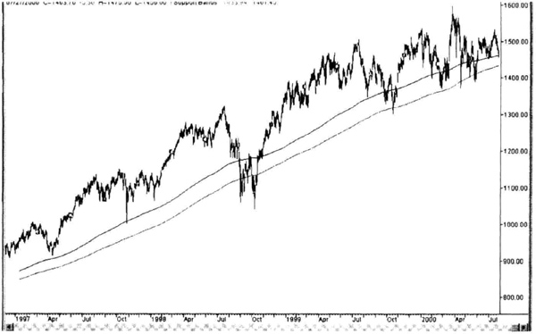
Figure 1.26 A continuous chart of the S&P-500 daily futures with 400-day simple moving average and bands set at one-half of the 400-day standard deviation of closing prices. The long-term support and resistance seem to lie near the bands.

Figure 1.27 The Eurex DAX futures contract found support at the 400-day moving average and the bands set at one-half the 400-day standard deviation of closing prices.

Figure 1.28 A continuous contract for New York Cotton showing resistance at the 400-day simple moving average during a multiyear downtrend.