
Genomics
Abstract:
The human genome is the blueprint of the human body. It encodes valuable yet implicit clues about our physical and mental health. Human health and diseases are affected by inherited genes and environmental factors. A typical example is cancer, thought to be a genetic disease, where a collection of somatic mutations drives the progression of the disease. Tracking the disease roots down to the DNA alphabet promises a clearer understanding of disease mechanisms. DNA alphabets may also serve as stable biomarkers, suggesting personalized estimates of disease risks or drug response rates. In this chapter, we explore techniques critical for the success of genomic data analysis. Special emphasis is placed on the adaptive exploration of associations between clinical phenotypes and genomic variants. Furthermore, we address the skillful analysis of complex somatic structural variations in the cancer genome. An effective use of these skills will lead toward a deeper understanding and even new treatment strategies of various diseases, as is evidenced by the case studies.
2.1 Introduction
The human genome underlies the fundamental unity of all members of the human family, as well as the recognition of their inherent dignity and diversity. In a symbolic sense, it is the heritage of humanity.
The human genome, the entire inherited blueprint of the human body, physically resides in every nucleated human cell. A rich content of genomic information is carried by the 23 pairs of autosomal and sex chromosomes, as well as the mitochondrial genome. Chemically, the human genome is a set of deoxyribonucleic acid (DNA) molecules, comprised of long strings of four basic types of nucleotides: adenine (A), thymine (T), guanine (G) and cytosine (C). The human genome comprises 3.2 billion nucleotide base pairs, where a base pair is either a G-C pair or an A-T pair, connected by a hydrogen bond. Genes and regulatory elements are encoded by the four nucleotides. A gene refers to a DNA sequence that can serve as a template for the assembly of another class of macromolecules, ribonucleic acid (RNA). The protein-coding messenger RNAs are produced according to the DNA templates in a process called transcription, which is also controlled by the upstream DNA sequence of the gene called the regulatory element.
Genomic DNA is largely identical among healthy nucleated cells, except for certain specialized immune cells and some harmless somatic mutations scattered throughout the genome. Therefore, it is accessible in many types of tissues of the human body. DNA has a double helical structure with two strands of DNA tightly bound by hydrogen bonds. As a result, DNA is a more stable molecule and more static than downstream mature RNAs (mRNA) and proteins, which are dependent on time, tissue expression and degradation patterns. Thus, it is a reliable material for the study of the molecular basis of clinical traits.
A haploid human genome (i.e. the DNA in one strand of the double helix) comprises 3.2 billion bases. Despite its sheer length, only 28% of it harbors the 21,000 protein-coding genes (IHGSC, 2004). The rest of the genome encodes regulatory functions, contains repetitive sequences (> 45%), or plays unknown roles waiting to be discovered. For example, a promoter region preceding a gene can serve as the site where the polymerase binds, regulating the transcription of this gene. The precursor RNA transcripts, directly transcribed from the DNA template, are subject to a splicing process before the mRNA is produced. Most of the precursor regions, called introns, are spliced out. As a result, only a small fraction (called exons, covering 1.1-1.4% of the genome) contribute to the final mRNA, which is further translated into proteins. Metaphorically, these protein-coding genes are analogous to archipelagos scattered in the wide open sea of the entire genome. The exonic regions are like the islands in an archipelago, which can give rise to mRNAs. The intron regions are analogous to the inner sea. The exons are then further categorized as 5’untranslated regions, protein coding regions, and the 3’untranslated regions, depending on whether or not they directly encode the protein sequence.
2.1.1 Global visualization by genome browsers
A sea is so large that even an experienced sailor needs the navigating tools of maps and compass to direct his exploration. Similarly, the deluge and richness of genomic information prohibit investigators from comprehension and analysis without the aids of computational tools. Computers are not only used to store, organize, search, analyze and present the genomic information, but also to execute adaptive computational models to illustrate the characteristics of the data. Visual presentations are crucial for conveying the rich context of genomic information in either the printed forms or the interactive, searchable forms called genome browsers. Here we introduce three commonly used diagrams for genomics. First, a karyogram (also known as an idiogram) is a global, bird’s eye view of the presentation of the 23 pairs of chromosomes and their annotations. For example, it can be used to present the tumor suppressor genes by showing their locations on the chromosome. One of the popular tools for producing a virtual karyogram is provided by the University of California, Santa Cruz (UCSC) Genome Bioinformatics site (Box 2.1).
Box 2.1 Bioinformatics resources and tools for genomics
GenBank, hosted in the NCBI (National Center of Biotechnology Information), is one of the most valuable resources of genomic information. It provides DNA, RNA and protein sequences through a spectrum of specialized databases. Some are designed with extensive curation aiming to provide only high-quality data (e.g. RefSeq). Others are focused on wide incorporation of exploratory data. The dbSNP database contains information about known SNPs. The NCBI site is one major place for newly discovered sequences to be submitted and deposited. The accompanying search engine is called Entrez, where users can locate information using sequence accession numbers (IDs) and key words. The default sequence alignment algorithm is BLAST, an algorithm combining heuristic seed search and dynamic program for alignment extension. NCBI also offers several valuable tools for experiment design, such as:
This is a web service or primer design based on primer 3, one of the most commonly used primer design tools. The Primer-BLAST has added-on, multiple and practically useful functions such as intron inclusion (an ideal feature to design primers for alternative splicing), exon-exon boundary check or exon-i ntron check. It also checks all the possible amplicons (PCR products) for a pair of primers from the database, including amplicons generated from the imperfect base pairing of the primers to the templates. This is a useful feature for the design of the primer, to avoid primers that can generate unwanted products.
This website is used to check the expected amplicon of a pair of primers. This is based on the blast sequence alignment against the built- i n genome and transcriptom database (i.e. RefSeq). This tool can be used to check whether the designed primer pair results in a multiple hit, and check whether the primer pairs will produce contamination, which is not to be pursued.
The UCSC Genome Bioinformatics site, hosted by the University of California Santa Cruz, contains complete and organized genomics data as well as many levels of annotations. It is best known for an interactive genome browser. It also provides a variety of information query methods. Furthermore, the sequence alignment tool BLAT is very efficient for database queries of homologous sequences.
HapMap is a series of population genomic studies of several ethnic groups worldwide. The website contains valuable information about SNPs and population specific allele frequencies. An interactive genome browser is provided on the website. Furthermore, Haploview (provided by the Broad Institute of MIT and Harvard) is a standalone software for viewing the haplotype data from HapMap.
SeattleSNPs, also known as the Genome Variation Server, offers a convenient online portal site for presenting, browsing and searching of SNP-related information such as LD. HapMap data can also be accessed here.
CIRCOS is a Perl-based platform useful for generating circular chromosomal maps. This software has been used extensively to generate high resolution, publication-quality presentation of genomic studies, such as somatic mutations or chromosomal rearrangements.
![]() ALLPATH, ALLPATH-LG and Velvat
ALLPATH, ALLPATH-LG and Velvat
ALLPATH and ALLPATH-LG offers de novo assembly tools for NGS readings. Velvat is also a de novo sequence assembler of NGS readings, hosted by EMBL-EBI.
Bowtie software offers the mapping of NGS readings of the long sequences such as the human genome. This software is downloadable from sourceforge.net. There are two major versions: Bowtie 1 (Langmead et al., 2009) and Bowtie 2 (Langmead and Salzberg, 2012). The latter offers local alignment and gapped alignment. Bowtie 2 is also faster and more sensitive than Bowtie 1, when the average sequence reading is larger than 50 bases.
Chromas Lite is a lightweight software for showing the analog chromatogram signals in the trace files and also produces base calls.
C Visual presentation and interpretation
WGAviewer is a standalone software, provided by Duke University, to present a series of GWAS P-values in Manhattan plots and also annotate the most significant SNP hits by connecting to online databases such as Ensemble and HapMap. The presentation is also facilitated by ideogram, Q-Q plot, the r2 values of a SNP with adjacent SNPs, and gene locations. The software is written in the JAVA programming language.
LocusZoom is a useful website service, provided by the University of Michigan, for presenting regional SNP association results with annotations (Pruim, 2010). This site incorporates data from several GWAS for demonstration and re-analysis. Users can also submit their own data for analysis and presentation. The default input format is PLINK. A stand alone version of the software, built upon Phython and R, is also available for linux platforms.
SNAP stands for SNP Annotation and Proxy search offered by the Broad Institute. It offers an LD plot, which can also show recombination sites. Data of the HapMap and the 1000 genome project are incorporated in the site. This can be used for the imputation of associations on unassayed variants, by the use of LD from the public domain data.
Octave is a free scientific computation package. It employs the scripting language of Matlab, another widely used commercial scientific computation package. Octave and Matlab are excellent for matrix and vector computations. They are also useful for visual presentation of 2-D and 3-D scientific data.
Second, a genome browser is an integrative, interactive visualization tool that can present genomic information, chromosome by chromosome, with multiple resolutions of annotations. Several genome browsers are part of important bioinformatic portals, for example, the Ensemble and HapMap websites (Box 2.1). A genome browser can also be standalone software, for example, the freeware “GenomeBrowse” offered by Golden Helix Inc. A genome browser usually has an interactive, zooming in and zooming out interface to navigate to regions of interest and adjust to the right scale/resolution. This enables the visualization of large-scale contexts and small-scale details. It also has multiple tracks, which can each be designated to a special type of annotation such as the exon and intron locations, personal variants (to be discussed later), splicing patterns and functional annotations. The presentation of multiple tracks simultaneously offers an integrative view of complex information.
A genome browser is traditionally designed as a linear, horizontal interactive graph with multiple layers of annotation showing simultaneously as tracks. With the current requirement of presenting complex gene interactions and structural variations across chromosomes, a new type of genome browser has been designed with a circular shape with the chromosomes forming the circle. Annotations are then represented in the circular tracks, and the interactions of loci are shown as arcs within the circle. Recently, such a type of genome diagram and browser was constructed by the CIRCOS software (Box 2.1).
2.2 The human genome and variome
2.2.1 Genomic variants
A substantial portion of the human genome is identical amongst people; the differences are called variants. Many such variants are scattered in the human genome. They can be classified, based on their lengths (scales), as:
![]() microscopic variants (> 3 mega bases, 3 M);
microscopic variants (> 3 mega bases, 3 M);
![]() sub-microscopic variants, such as copy number variations (CNVs); and
sub-microscopic variants, such as copy number variations (CNVs); and
![]() small variants (< 1 kilo bases, 1 kb), including single nucleotide polymorphisms (SNPs), point mutations (single-base substitutions), short tandem and interspersed repeats (Feuk et al., 2006).
small variants (< 1 kilo bases, 1 kb), including single nucleotide polymorphisms (SNPs), point mutations (single-base substitutions), short tandem and interspersed repeats (Feuk et al., 2006).
The collection of all variations found in the human population is called the human variome.
The single-base SNPs and point mutations are important classes of genomic variants, partly because of their sheer numbers. Large-scale human genome sequencing projects, such as the 1000 Genome Project and the uk10k Project (a 6000 vs. 4000 case vs. control study aiming to conduct the sequencing of the protein-coding regions), have increased the SNP count to 20 million (Pennisi, 2010). Both SNPs and point mutations have two (occasionally three) alleles: the more common one is called the major allele, while the less common one is called the minor allele. A SNP is defined as having a minor allele frequency (MAF) higher than 1% in a population. The International HapMap Project has achieved a valuable database that can be used to calculate allele frequencies across populations (The International HapMap Consortium, 2007; Altshuler et al., 2010). The HapMap Project is prioritized to collect common variants with MAF higher than 1%. The core of the database is a large SNP-by- s ubject matrix of genotypes. The Phase 3 collection contains genotypes of 1,600,000 SNPs of 1184 subjects in 11 populations. The database has many uses, such as the comparison of allele frequencies in different ethnic groups and the demonstration of genomic structure based on correlations between SNPs.
On average, there is 1 SNP in every 150 nucleotides (20 million SNPs scattered in a 3 billion nucleotide genome, see Table 2.1). Hence, SNPs offer dense genomic markers. Each SNP has a unique position in the genome and is assigned a unique identification (ID) by dbSNP, one of the most important resources of SNPs hosted by the National Center for Biotechnology Information (NCBI) site (Box 2.1).
Table 2.1
Information of various projects and technological platforms measured by numbers of nucleotide bases
| Item | Bases |
| The human genome | 3,000,000,000 |
| Known total SNPs | 20,000,000 |
| Estimated number of SNPs with MAF > 10% | 7,000,000 |
| HapMap Phase 3 SNPs | 1,600,000 |
| Affymetrix 6.0 SNPs | 900,000 |
| Illumina HumanHap 650Y | 650,000 |
| Illumina HumanHap 550 | 550,000 |
| Affymetrix 5.0, 500k | 500,000 |
In addition to SNPs and point mutations, short tandem repeats and interspersed repeats are commonly found in the human genome. Alu is a class of primate specific, short interspersed repeats, which constitutes approximately 10% of the human genome (Lander et al., 2001; Decerbo and Carmichael, 2005). Cellular roles of Alu have been obscure and it was once thought of as junk DNA (Muotri et al., 2007; Lin et al., 2008). Alu can be found in intergenic regions as well as the coding and non- coding regions of many genes in either the sense or antisense strand.
Recent studies on human genome analysis have revealed a common class of germline variants, the CNVs that belong to a more general class called structural variants. The genome is thought to be diploid where one copy is from the father and one from the mother. Yet, on the sub- microscopic scale, multiple genomic regions exhibit multiple elevated (e.g. above 3 copies) or reduced (e.g. 1 or 0 copies) numbers of copies, and are called CNVs. These are common, mostly harmless variants, although some have been linked to disease. The shortest length of a CNV is 1 kb based on its definition, yet many of them are longer than 100 kb. It is estimated that an average Asian person has 20 to 30 CNV loci in their genome, with an average size of 14.1 kb (Wang et al., 2007).
Cohorts of subjects need to be recruited to reveal the basic characteristics of genomic variants, such as total number and population frequency. The HapMap Project is a good example. In addition, we also need to find the genomic variants responsible for individual variability in disease susceptibility or drug response. This can also be achieved by genomic studies with adequate sample size, rigorous statistical measures, and unambiguous definition and recruitment of subjects with distinct clinical phenotypes.
Somatic mutations of various scales play significant roles in the etiology of many illnesses, particularly cancer. Most cancers originated from somatic cells transformed via a series of genetic or epigenetic modifications during the aging process (Luebeck, 2010; Stephens et al., 2011). These cells gradually exhibit many abnormal capabilities such as anti-apoptosis, tissue invasion and metastasis (Gupta and Massague, 2006). Somatic mutations of oncogenes or tumor suppressor genes could serve as important biomarkers in various stages of cancer biology. In terms of treatment, traditional chemotherapy agents have been designed against fast dividing cells. The more recent target therapies employ antagonists to various oncogenes directly. Cancer patients show varied responses, chemotherapy or targeted therapy alike, because their cancer cells are at different stages and with various features and capabilities. This is why the optimum treatment strategies differ. Studies of somatic mutations on targeted genes, oncogenes and tumor suppressor genes may be able to identify the best treatment strategy for each individual.
2.2.2 A multiscale tagging of your genome
Linkage disequilibrium (LD) is a unique feature among genomic variants. It refers to the association of genotypes between adjacent variants. It is a direct consequence of chromosomal recombination (also known as crossover), which occurs during meiosis for the production of germ cells. Where there are no chromosomal recombinations, all variants in one chromosome should be tightly associated to each other, as they are passed down together to future generations. A chromosomal recombination disrupts the association (and introduces independence) between variants at the two sides of the recombination spot. After several generations, distant variants are no longer associated due to many recombination hotspots between them. The adjacent variants still retain a certain degree of LD, particularly those between two recombination hotspots. LD of a pair of variants can be quantified by r2 or D’ values. r2 is a value between 0 and 1, while 0 indicates no association and 1 indicates high association. LD can be shown as LD-heat maps by the Haploview software or the SeattleSNPs site (Box 2.1).
LD is a cornerstone for the design of genotype vs. phenotype association studies. Since many variants are adjacent to the causative variant, their genotype may also be in LD with the causative genotype. In the results of many high density association studies, we have seen multiple adjacent SNPs associated to the clinical trait simultaneously. The concept of using adjacent variants to serve as surrogates can alleviate the burden of finding the exact causative variants directly. We can first detect the surrogates, then scrutinize the proximity region of the surrogate to find the real causative variant. In practice, this is realized by the selection of representative SNPs (known as tag SNPs) in the study design phase, assuming the true causative variant is in LD with the tag SNPs.
A variety of tagging software is available based on r2 LD statistics (Box 2.1). For example, a tag SNP selection software, called the LDSelect method, has been implemented for data organization and analysis on the SeattleSNPs website (Carlson et al., 2004). LDSelect can ensure the selected tag SNPs have relatively low LD between each other, thereby minimizing the number of SNPs while maximizing their representativity. The FastTagger is a GNU GPL open source software (Liu et al., 2010). It implements two tagging algorithm, MultiTag and MMTagger. FastTagger comprise two consecutive steps:
Tagging is conventionally applied to a chromosomal region, with a fixed window size, due to computational limitations. By extending the concept of tagging from one layer into multiscale tagging, we can achieve the tagging of genome-wide variants. This can be achieved by a bottom-up layer construction approach (Figure 2.1). The entire set of genomic variants is defined as layer 0. We then tagged on top of layer 0, using a defined r2 threshold and a window size, to produce layer 1 containing only the tagged variants. The tagging reduced the number of variants in layer 1 compared with layer 0. A hierarchical structure can be further constructed, layer by layer iteratively, with an increasing window size. Every layer comprises the tagging SNPs of the immediately lower layer. After a few iterations, the top layer is constructed, serving as a reasonable representation of genome-wide variants.
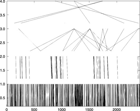
Figure 2.1 A five-layer multiple scale tagging structure of chromosome 22 when r2 = 0.4. The x-axis shows SNP indexes sorted by chromosomal positions. The y-axis represents the layer number. Chromosome 22 is defined as layer 0. Each layer is constructed iteratively by the tagging process of SNPs of the immediate lower layer. Lines in the graph represent the relationship between taggers in the upper layer and taggees in the lower layer. The distance between taggers and taggees increases as the layer increases, due to increasing window size. (The figure was produced by Octave.)
2.2.3 Haplotypes
The complex disease common variant (CDCV) hypothesis has been the underlying hypothesis of mainstream genome studies in the first decade of the 21st century (Goldstein, 2009). It influences many genome-wide association studies (GWAS) and early phases of the HapMap Project. This hypothesis assumes that complex disease is more likely to be caused by SNPs with higher MAFs (i.e. common alleles) than rarer SNPs and mutations. Therefore, higher priority is given to the searching, genotyping and disease association of common SNPs. But how about the rarer SNPs, mutations and other types of rare variants, which are also likely to be responsible for many diseases? Apart from using next generation sequencing (NGS) to capture all of them, an alternative way to accommodate them is by employing the concept of haplotypes.
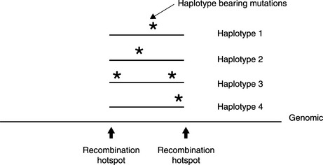
The human genome comprises two haploid (i.e. single copy) genomes, one from the father and one from the mother. When we perform conventional genotyping, we usually obtain diploid information, without distinguishing which is from the father and which is from the mother. For example, the “C vs. T” SNP of a person could be one of three diplotypes: CC, CT and TT. A haplotype block is a chromosomal region between two recombination hotspots. Haplotypes are alleles physically residing in a haplotype block of the same haploid chromosome, also called the phase of the genome, as opposed to the “unphased” diplotypes. Since the variants in a haplotype block are assumed to be inherited together, it is possible that a haplotype allele may carry an untyped, disease-causing variant. By analyzing the association between haplotype and the disease trait, we indirectly find the disease-causing variant (Figure 2.2).
A haplotype analysis has many steps:
Determine haplotype blocks
The haplotype block of interest can be identified between two recombination hotspots. This is based on the high LD among the variants (usually common SNPs) within the region.
Haplotyping
Given a cohort of subjects, the diplotypes of the variants are used for computational phasing (also known as haplotyping) to resolve the phase of the haplotypes. Given a haplotype block of n bi-allelic SNPs within a block, the resolved haplotype number will be much smaller than 2n, due to the LD between the SNPs. Computational phasing can be carried out by software such as Phase2 or THESIAS (Tregouet and Garelle, 2007) (Box 2.1).
Haplotype association
The haplotype frequency is calculated based on the haplotype counts of the case and control groups. If there is a significant difference between the two groups, then an association is found (Liang and Wu, 2007).
Haplotypes have shown tremendous value in another application: handling mixture genomes. One example is to reconstruct the fetus genome from pregnant women’s peripheral blood samples (Kitzman et al., 2012; Fan et al., 2012).
2.3 Genomic platforms and platform level analysis
Genomic studies begin with the acquisition of genomic sequences and their variants, such as point polymorphisms, mutations, copy number alterations and genome rearrangements. The nucleotide bases of DNA and RNA not only contribute to the basic material for genomics and transcriptomics, but also infer theoretical protein sequences, which have a wide use in many aspects of proteomics studies. The NGS platforms and high density SNP arrays are two major high throughput platforms to generate the genomic data.
2.3.1 Capillary Sanger sequencing and next generation sequencing
Conventional capillary sequencers employed the Sanger methodology and served as the major contributors of the human genome project. This method has limitations on sequence reads (~ 1000 bases), which is far shorter than the genome of most species. Thus, sequencing of genomic DNA needs to start by breaking the DNA macromolecule into smaller pieces. Sequencing is then performed on the pieces. The final step is to computationally or manually stitch the pieces together into a complete genome, an inverse problem called assembly. NGS platforms, so-called because of their relative advancement of conventional capillary sequencers in terms of higher speed and lower cost, have been made commercially available. Major vendors (and platforms) include Illumina (Solexa), Roche (454) and Applied Biosystems (SOlid).
However, NGS produces shorter sequence readings than conventional capillary sequencing. The strength of NGS (speed and lower cost) enables a mass production of readings, resulting in deep sequencing with high coverage (i.e. 100x), which may compensate for the weakness of shorter readings. It has been shown that the sequence readings of commercial NGS platforms can be used for the de novo assembly of human genomes (Butler et al., 2008; Gnerre et al., 2011). NGS can also be used to detect germline and somatic point mutations, copy number alterations and structural variations. With the launch of NGS, large-scale genomics investigations now employ NGS in the interest of speed and cost. Conventional capillary sequencing is reserved for small-scale studies. Sequencing technology is still advancing so that new technology (i.e. nanopore) is continuously being developed, so as to reduce the cost and increase the efficiency of sequencing even further.
Base calling for capillary sequencing
The output of capillary sequencers are chromatograms, which are four- channel analog signals representing a digital sequence of nucleotides A, T, G and C. Chromatograms are commonly stored in trace files. Base calling is the very first step to convert the analog signal into digital nucleotides. A series of software, phred, phrap and consed, has been widely used for handling chromatograms from capillary sequencers. They also serve as the basis of bioinformatics pipelines in many genomic centers (Box 2.1). The phred software is designed to call bases, in the meantime providing a quality score for each base, which is informative for subsequent analysis such as assembly and small- scale variant detection (Ewing and Green, 1998; Ewing et al., 1998). Phrap is a sequence assembler that stitches sequence readings from phred. Consed is a program for viewing and editing phrap assemblies. Software such as Chromas Lite and UGene can be used to visualize the trace files and also produce base calls from them (Box 2.1). The above two software packages do not handle variants (i.e. SNPs in the diploid genome), because the computation is based on the assumption that no heterozygous bases occur in the sequences. Where the variants in sequences are of concern, more advanced software for handling variants should be used.
Base calling for NGS
This is often taken care of by the vendor software, which converts analog signals (image intensities) into digital sequence readings directly. All subsequent analysis relies on these readings.
Variant detection
Detection of small-scale germline or somatic variants can be by the concurrent analysis of multiple samples in the same sequence region. Several high-quality software packages, such as PolyPhred, PolyScan (Chen et al., 2007), SNP detector (Zhang et al., 2005) and NovoSNP (Wecks et al., 2005), are designed for such a purpose (Box 2.1). NovoSNP has an excellent graphical user interface and is suitable for personal use. It can conveniently align multiple trace files so that the candidate variants can be compared across sequences. Polyphred, polyscan and SNP detectors rely on phred for individual base call and quality scores. For example, the integrated pipeline PolyScan is designed to call small insertions and deletions as well as single base mutations and SNPs on multiple traces. It requires not only the called bases but also the quality scores from the phred software and the sequence alignments from consed. The bases are designated again by four features extracted from the trace curves: position, height, sharpness and regularity (Chen et al., 2007). Bayesian statistics are used for the inference of variants.
2.3.2 From sequence fragments to a genome
Assembly
Genome assembly is an important technique to stitch together the sequence readings from sequencers into chromosome-scale sequences. This is how reference genomes (including human) are built. Reference sequences are of tremendous value in all aspects of biology. Once they are built, all the following sequencing tasks of the same species (called re-sequencing) can make use of the reference sequence. The sequence readings can be mapped to the reference using an aligner such as Bowtie (Box 2.1). When a reference genome is unavailable, then direct assembly from sequence readings (called de novo assembly) is still required for organizing sequence readings.
Mathematically, a de novo assembly of genomic sequences is an inverse problem. The performance of a de novo assembly of a genome needs to be gauged by several aspects, including completeness, contiguity, connectivity and accuracy. To understand these, we need first to define “contig” and “scaffold”. A contig is a continuous sequence (without gaps) assembled from sequence readings. A scaffold is formed by contigs with gaps of known lengths between the contigs. The contiguity and connectivity can be shown as the average lengths of contigs and scaffolds respectively; the longer, the better. The completeness of contigs and scaffolds is the proportions of the reference genome being covered by contigs and scaffolds (including gaps) respectively. The accuracy means the concordance of bases in the contigs and the reference genome (Gnerre et al., 2011).
DNA fragments to be assembled have several types. The first types are the typical fragments, which are usually shorter than twice the average read lengths. By sequencing the fragments from both ends, an overlapped read region can occur in the middle to join together the two ends, resulting in a single fragment sequence. For example, if the read length is 100 bases, then fragments of 180 bases (shorter than 200 bases) can be unambiguously sequenced. A high volume of fragments can serve as the foundation of assembly of simpler genomes.
Repetitive regions occur in a complex genome such as human and mouse. To overcome the challenge of assembling such genomes, longer fragments of a few thousand bases may be required. This can be done by a mate pair strategy to fuse the two ends of the long fragments (e.g. 3000 bases) to produce a circular DNA, then shatter the DNA into smaller pieces. Since the original two ends are now joined together, they can be sequenced to provide “pairs” of sequences with a longer distance between them. These are called “jump” sequences.
Phrap is one of the pioneering sequence assemblers, which can handle the assembly of readings from capillary sequencers well. As the NGS now produces much shorter readings than conventional capillary sequencing, a new generation of assembler is required. Despite challenging, it has been shown that de novo assembly of the repeat rich human genome can be achieved using shotgun NGS reads (Gnerre et al., 2011). The shotgun approach means that genomic DNA is randomly shattered. The assembly of these readings into longer contiguous sequences (called contigs) all relies on computational approaches without knowing of their genomic location beforehand.
ALLPATH-LG is a de novo assembly algorithm adapted from the previous ALLPATH algorithm (Butler et al., 2008). ALLPATH-LG was specially tuned for the sequencing of both human and mouse genomes (Box 2.1). It starts by constructing unipaths, which are assembled sequences without ambiguities, then tries to localize the unipaths by joining them together using long “jump” sequences. The human and mouse genome has been shown to be assembled by the same algorithm using the same parameter, suggesting its potential for the genome assembly of other similar species with minimal tuning.
Alignment
Sequence alignment is one of the most extensively discussed bioinformatics topics, which have been the core skill for experimental biologists and professional bioinformaticians alike. It appears in many applications such as the construction of the evolutionary tree or database searches. There are two major types. The “local” sequence alignment aims to find a common partial sequence fragment among two long sequences. The common partial sequences may still have differences in their origins such as insertions, deletions and single-base substitutions. However, the historically earlier “global” sequence alignment is employed to align two sequences of roughly the same size.
The public domain databases, such as NCBI GenBank and EMBL, contain invaluable DNA, RNA and protein sequences of multiple species such as human, rice, mustard, bacteria, fruit fly, yeast, round worm, etc. The sequences are generated by scientists worldwide for many purposes. The NCBI RefSeq database contains curated, high- quality sequences (Pruitt et al., 2012). Public archives often provide many ways to browse through or search for the information contents, and one of the major search methods is by sequence alignment. Finding similar sequences by alignment is of interest, because similar sequences or fragments usually imply similar functions due to their common evolutionary origin. The current model of evolution describes that every organism has originated from a more primitive organism. If a genome duplication event occurs in an ancient organism, then genes in the duplication region will be copied. Each copy of a gene may evolve gradually. It might become a pseudo gene and lose its functionality, or become a new gene with similar functionality. Then these genes are passed through the lineages.
In the past, many algorithms have been proposed for sequence alignments. For example, Needleman–Wursh and Smith–Waterman algorithms are classic examples of global and local sequence alignment respectively. They both employ the dynamic programming approach for optimization. BLAST (Basic Local Alignment Search Tool) is the most widely used method combining a heuristic seed hit and dynamic programming. There are other methods, such as YASS, which employ more degrees of heuristics (Noe and Kucherov, 2005). It is important to know that different algorithms have different characteristics, such as speed and sensitivity.
BLAST is the default search method for the NCBI site. A user can provide a nucleotide sequence of interest by typing in a dialog box, or by submitting a file containing the sequence. After only a few minutes of computation, the system produces a bunch of hits, each of which represents a sequence in the database that has high similarity to the target sequence. If the user clicks on a particular hit, then more details of this sequence will appear.
A variety of indexes are displayed for a particular hit, for example, IR stands for identity ratio, which indicates how much percentage per base is this sequence from the database to the sequence of interest. The e-value stands for expectation value, which is the expected number of coincidence hits given the query sequence and the database.
Many aspects in the system significantly affect the practical usefulness and users’ experience in addition to the underlying algorithms. These include visual presentation, scope, completeness and up-to-date information of the database. Certain specialized functionalities can enhance the usefulness greatly. The SNP BLAST site, also provided by NCBI, is such an example. The users still submit the sequences as on the regular BLAST site, but instead of a list of matched sequences, the system reports a list of SNPs and their flanking sequences matched to the submitted sequences. This is particularly useful to identify the location of the submitted sequence in the genome, by means of the high resolution genomic markers. This is also useful for checking the amplicon of the genotyping via sequencing method.
Multiple sequence alignment is used to find the conserved area of a bunch of sequences from the same origin. These sequences are of the same gene family. The conserved area, normally called motifs and domains, is useful in characterizing a gene family.
Sequence alignment can be achieved on-line by using a variety of website services. It can also be done off-line using the downloaded software.
Annotation
When a genome of a species is newly sequenced, it is important to decode the message encoded by the sequence. The sequence structure of a gene is like a language, which can be processed using information technologies. High-quality annotations on the sequences are important to unveil the “meaning” of the sequence’s gene prediction. Open reading frame prediction and gene prediction are useful for genome annotation. Some previous works include the use of a hidden Markov model for gene prediction.
2.3.3 Signal pre-processing and base calling on SNP arrays
High-density SNP arrays are the major tool of assessing simultaneously the genome-wide variants and CNVs. Based on intensity profiles, the arrays can be used to detect germline and somatic CNVs, where the unusual copy number (other than the two paternal and maternal copies) is shown as increased or decreased intensity signals. In addition to SNP arrays, array CGH is another major platform to detect the CNVs, particularly the loss of heterozygosity in cancer tissues.
Affymetrix and Illumina are two leading commercial manufacturers and vendors of high density SNP arrays. The latest Affymetrix SNP 6.0 microarray product has 1.8 million probe sets targeting 1.8 million loci evenly scattered in the genome (Table 2.1).
Among them, 900,000 are designed to assay SNPs and 900,000 for CNVs. When the number of SNPs is large (e.g. > 100), the high- density microarrays have many practical advantages over various conventional single SNP assays. The latter requires a special set of primers for each SNP. This is not only costly and time-consuming, but also complicates the whole experimental process, including the logistics of reagents and management of data. A good bioinformatics system is essential to keep track of data. Finally, unnecessary variability may be introduced when each SNP is handled at different times and by different persons. A high-density microarray can assay thousands of SNPs in one go, reducing the complexity, cost, time and variability significantly.
High-density SNP microarrays contain pairs of probes designed to capture pairs of DNA sequences harboring the major and the minor allele types respectively (i.e. the target sequence). Existence of a particular genotype in the sample will be detected by the signal of hybridization of the probe corresponding to the target sequence. Hybridization will be shown as intensity signals, which are captured by a scanner and stored as digital images. Raw images usually need to be pre-processed, using background subtraction and normalization techniques (for details, see Section 3.3 in Chapter 3), so as to compensate between array variations. The quantitative intensity signal will then be converted to binary showing exist (1) or non-exist (0) of the allele type in the sample, that is, the base calling process. This is a critical process for reading out nucleotide bases from analog signals.
Many unsupervised and supervised algorithms have been proposed for base calling, such as DM, BRLMM, BRLMM2, Birdseed, Chiamo, CRLMM, CRLMM2 and Illuminus. Since the most recent platforms are capable of detecting structural variations together with SNPs, software such as Birdseed can analyze SNP and CNV at the same time.
The handling of sex chromosome (X and Y) data requires special care compared with autosomal chromosomes. Females have two X chromosomes while males have an X and a Y chromosome. Hence, males only have one allele on X (i.e. hemizygous) and the other “missing” allele can be considered as a null allele (Carlson et al., 2006). Since the null allele may affect the base calling performance when a batch of samples contain both males and females, special algorithms have been developed to handle such occurrences (Carlson et al., 2006). Null alleles may also occur in deletion regions of autosomal chromosomes (Carlson et al., 2006).
2.4 Study designs and contrast level analysis of GWAS
2.4.1 Successful factors
Association studies are frequently used to find genes responsible for various clinical manifestations, such as the onset and progression of disease, as well as therapeutic efficacy and toxicity. Association studies were once carried out in a candidate gene fashion, yet now are predominantly done by GWAS. GWAS has successfully identified dozens of novel associations between common SNPs and various common diseases (Hirschhorn, 2009). The knowledge gleaned from these studies is invaluable for the further advancement of biomedical science. Despite some initial success, it was found that most risk alleles have moderate effects and penetrance, preventing them from direct use in personalized healthcare. One of the lessons learned from previous studies is that a well designed study is very important for achieving results. Factors for successful association studies include:
![]() clinically distinct study groups clearly defined by stringent criteria (deep phenotyping);
clinically distinct study groups clearly defined by stringent criteria (deep phenotyping);
![]() a strong contrast on targeted phenotypes between study groups: the supercase-supercontrol design;
a strong contrast on targeted phenotypes between study groups: the supercase-supercontrol design;
![]() a negligible contrast on other phenotypes between study groups: no confounding effects;
a negligible contrast on other phenotypes between study groups: no confounding effects;
The purpose of all the above factors is to ensure that the detected associations truly represent the clinical trait. A clear and strong contrast in phenotype (i.e. the supercase vs. supercontrol design) could enhance the contrast in genotype, thereby enhancing the possibility of success of finding potential biomarkers, particularly at the exploratory stage. We need to note that the odds ratio (OR) detected does not reflect the true OR in the epidemiological scenario. The hidden population heterogeneity can generally be detected by the inflation factor (Freedman et al., 2004). In such cases, population filters (discussed below) are important.
Many meta-analyses of GWAS have shown that a larger sample size can improve results in terms of both the number of detected SNPs and their significance. For example, a meta-analysis of 46 GWAS with a total of more than 100,000 subjects captured all the 36 originally reported associations, while discovering 59 new associations to personal blood lipid levels (Teslovich et al., 2010). It was found, however, that SNPs on major disease genes of familial hypercholesterolemia were also detected, blurring the conventional categorization of familial diseases vs. common diseases.
2.4.2 The data matrix and quality filters
Association studies are widely used to find the hidden relationship between genetic variants and clinical traits of interest (WTCCC, 2007). In practice, an association study is designed to compare the allele frequencies of two groups with distinct clinical status: the case group comprising subjects with the clinical trait of interest (e.g. a disease state or a therapeutic response) and the corresponding control group. The study subjects are often collected retrospectively, but can also be recruited prospectively. A prospective study means that the clinical outcome is manifested after the samples are collected and assayed (Patterson et al., 2010). The underlying concept for an association study is that genotypes which cause a clinical trait, directly or indirectly, will be more enriched in the case groups, producing a difference in allele frequencies.
In the past, association studies were done by the candidate-gene approach that scrutinizes a targeted set of genes, which is hypothesized to exert effects on disease etiologies based on prior knowledge. This approach has gradually been replaced by GWAS, which is done in a holistic perspective and hypothesis free style with all known genes screened in an unbiased fashion. This was enabled only recently by the maturation of commercial high density SNP assaying platforms such as Affymetrix SNP 6.0 arrays. These platforms were designed for assaying SNPs with not-so-rare minor alleles (e.g. MAF > 0.1), a consequence of the “complex diseases common variant” hypothesis widely accepted before 2009 (Goldstein, 2009). A GWAS usually screens 100,000 to 1,000,000 SNPs, a reasonable sub-sampling of the entire set of genomic variants (Table 2.1).
A conventional master file of an association study is a subject-by-SNP data matrix, comprising genotypes in multiple SNPs of multiple subjects. The genotypes of all subjects are converted from the scanned intensity of SNP microarrays or from the sequencing trace files using the corresponding base calling software. The subjects are sorted by clinical status for ease of comparison. The SNPs are preferably sorted by the chromosomal locations. The subject-by-SNP data matrix is denoted as D, where the subjects are categorized as cases or controls. Each row of D represents a sample of a subject (person), and each column represents an SNP. Denote n as the total number of SNPs, therefore, D = {SNPj | 0 <= j < n}. The subject-by-SNP matrix is part of a PLINK format. It can be visualized using colors, as in the SeattleSNPs presentation. In some data formats. such as the Oxford format, FastTagger and Slide, the SNP-by- subject is used instead. Considering the 100,000 to 1,000,000 SNPs screened in a GWAS, the dimension of the dataset appears to be huge. Yet, the underlying correlation between adjacent SNPs is a biological feature known as LD, which can effectively reduce the complexity of the data matrix.
A collection of quality filters is usually applied to the data matrix, prior to or after the statistical analysis, to ensure the results are derived from high-quality data and reflect the genuine biological effects. These filters are usually imposed in the following order:
a) Population filter: remove subjects (persons) from the dataset who belong to a population other than the study population. The population of a subject can be known from self-reported information, or by the analysis of genome-wide genotypes.
b) Sample or microarray quality filter: remove samples (microarrays) showing abnormal intensity distribution.
c) By call rate per subject: the number of called SNPs must be greater than a threshold such as 95% (Tanaka et al., 2009).
a) Base calling quality: remove SNPs that demonstrate abnormal intensity distributions, which render low-quality scores detected by the base calling algorithm.
b) Call rate per SNP: number of subjects which were successfully called in this SNP needs to be greater than a threshold such as 95% (Tanaka et al., 2009). This is particularly critical in the sense that problematic SNPs usually give a strong but false significance if not filtered previously. The problematic SNPs usually have abnormal signal distributions, which are difficult for base calling. That is why the call rate is usually low.
c) Hardy–Weinberg equilibrium test in the control group (optional for case group): SNPs that deviate from the Hardy-Weinberg equilibrium are removed. The Hardy-Weinberg equilibrium means that the observed genotype counts are close to the expected genotype counts calculated from observed allele frequencies. Whether the Hardy–Weinberg equilibrium is deviated from can be calculated using Chi-square tests. This is usually applied to the control (healthy subjects) group only (Minelli et al., 2008).
d) Association of nearby SNPs (optional): This is done after the calculation of association. This is based on observations that the risk locus usually manifests itself as multiple adjacent hits due to their LD (WTCCC, 2007). If the association is a singleton, which may be due to some artifacts rather than real biological effects, they are thus removed.
The data matrix could therefore contain missing data (blanks) due to the limitation of the base calling algorithm (the null calls) or the sample quality (filtered out by the quality filters). A small degree of missing data will be tolerated and will not hamper the analysis. Nevertheless, we can also choose to employ imputation algorithms to fill in the missing data, or un-genotyped SNPs, based on the LD structure of the SNPs. Imputation algorithms are particularly useful on the meta-analysis of GWAS employing different platforms, for example, Affymetrix and Illumina arrays, where the assayed SNPs are not identical and need to be imputed.
2.4.3 Contrasts of genotypes of individual SNPs
SNPs manifesting strong contrasts of allelic or genotypic frequencies between the clinical groups are pursued in an associations study. Two important gauges for every candidate association are:
The first gauge is the significance level, also known as the P-values, of statistical tests. The P-values quantify the probability of rejecting the null hypothesis when there is no association; that is, the probability of a false positive. Hence, the smaller the P-value, the higher the statistical significance. SNPs with P-values smaller than a predefined threshold (commonly set at 0.05 when only one variant is assessed) are confidently associated to a particular trait of interest. The second gauge is the ORs.
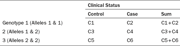
Both P-values and ORs are calculated from the counts of different allelic and genotypic forms. The 2 × 2 and 2 × 3 contingency tables are usually employed to present the counts (Tables 2.2 and 2.3).

Association tests include the allelic, genotypic and trend tests, which can be formulated either as a Chi-square test or a Fisher’s exact test. These tests are used to detect three types of risk patterns, the additive, dominant and recessive modes. Allelic tests evaluate the difference of allelic frequencies between the case and control groups. A related trend test aims to examine the increasing or decreasing trends of diseased frequencies (i.e. proportion of subjects who are the case group) in response to the addition of risk alleles. Allelic and trend tests basically evaluate the additive effect of each risk allele, in the sense that genotype 3 of two risk alleles will have twice the effect as genotype 2 with only one risk allele, thus the relationship between alleles and disease frequency is approximately linear. However, genotypic tests evaluate the difference of genotype frequencies between the case and control groups. Genotypic tests have three variants:
1. a comparison of three genotypes;
3. grouping genotypes 1 and 2 together, to be compared with genotype 3 (representing a recessive mode of inheritance);
4. grouping genotypes 2 and 3 together, to compare with genotype 1 (representing a dominant mode of inheritance).
Since the human genome is diploid, an unphased genotype (i.e. the diplotype) contains two alleles. Hence, the total allelic count is twice as large as the total genotype counts. This makes the allelic test double the sample size than the genotypic tests.
For example, the mathematical equation for a Chi-square allelic is: the Chi-square value (X2)
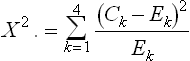
where
and the degrees of freedom is 1.
ORs are the ratio of odds with and without a particular allele or genotype. They can be formulated as:
Under the same formula, OR has many meanings, depending on the definition of G and ~ G. An odds ratio could mean:
The corresponding definitions of G and ~ G are
![]() G is an allele, while ~ G is the other allele;
G is an allele, while ~ G is the other allele;
![]() G is an genotype, while ~ G represent the other two genotypes;
G is an genotype, while ~ G represent the other two genotypes;
![]() G represents two genotypes, while ~ G is the other genotype;
G represents two genotypes, while ~ G is the other genotype;
It is thus important to check the definition before interpreting a result from the literature, particularly when multiple research works are compared. For example, the ORs in Tanaka et al. (2009) are the dominance mode, while those in WTCCC (2007) are heterozygote and homozygote ORs.
2.4.4 Sample size and multiple comparisons
When genome-wide variants are evaluated in parallel, multiple hypotheses testings, one per a variant, are performed. This comes with the cost that we must tighten the stringency on P-values for each hypothesis. This is called the issue of multiple comparisons. In such types of study, we need to control the family-wise type 1 error rate of the entire study. A common way to address the family-wise error rate is to employ Bonforroni corrections. For example, if n SNPs are assayed in a GWAS, and we want to control the family-wise error rate below 0.05, then each SNP will have an individual P-value smaller than 0.05/n before it can be declared statistically significant. For an Affymetrix SNP6.0 microarray with 900,000 genome-wide SNPs, significance level per SNP based on Bonforroni correction is 5*10−8.
In the Bonforroni correction setting, n represents the number of independent tests. However, due to the LD between adjacent SNPs in the human genome, hypothesis testings on these SNPs are not independent. Therefore, the conventional Bonforroni correction is often too conservative and inadequate. This can be mitigated by two approaches.
First, a permutation test is a non-parametric alternative that can take LD into consideration. It uses empirical permutation to calculate family-wise error rates, therefore requires a heavy computation which needs to be overcome, particularly in GWAS settings. Permory is a good software of permutation tests on GWAS datasets (Pahl and Schafer, 2010).
Second, prior domain knowledge can be used to devise filters and integrators (Ideker et al., 2011) and reduce the number of independent tests. Filters are used to remove poor-quality data and variants unrelated to the study. Integrators can be used to group variants into higher-order entities such as genes or pathways.
The sample size of this study depends on five factors. The first is the expected effect size of associations, often quantified by ORs. The second issue is the MAF. The range of MAF of SNPs is between 0.01 and 0.5. The third factor is the significance level considering the multiple comparison issues. The fourth factor is statistical power, which is usually set at 80%. The fifth factor is the ratio of the two clinical groups to be compared.
2.4.5 Visual presentation and interpretation
A contrast level analysis of GWAS data will derive a series of P-values for hundreds of thousands of individual SNPs scattered in all chromosomes. A Manhattan plot is a scatter plot that offers a useful grand-scale visualization of the GWAS result. The assayed SNPs are sorted by chromosome locations in the x-axis. The y-axis shows the negative logarithm of P-values, and as a result the higher dots represent significant hits. Freeware, such as WGAviewer (Ge et al., 2008) and Goldsurfer2 (Pettersson et al., 2008), as well as commercial software such as Golden Helix, can be used to produce a Manhattan plot (Figure 2.3).
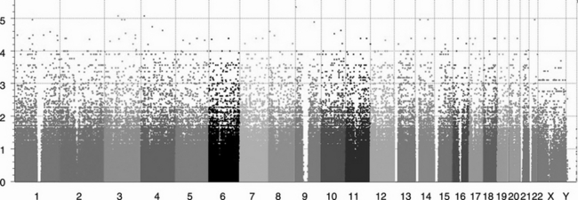
Figure 2.3 A typical Manhattan plot for a GWAS. The assayed SNPs are sorted by chromosome locations on the x-axis, with different chromosomes showing different colours. The y-axis shows the negative logarithm of p-values; as a result the higher dots represent significant hits. (The plot was produced by Golden Helix.)
GWAS and its subsequent validation render a short-list of SNPs, which are statistically associated to clinical traits. Albeit intriguing, the molecular mechanisms behind the associations are still vague. Thus, it is essential to pursue further functional exploration of detected associations. The first step is an in silico check of the SNP (variant) location in relation to the genes and the local LD pattern. Genome browsers in the RefSNP, dbSNP or HapMap websites can help users to locate whether the SNP is in the exon, intron or intergenic regions. If the SNP is located in the intron, then the databases H-DBAS or EBI-ASTD can be used to scrutinize the alternative splicing patterns. H-DBAS can also illustrate whether the SNP is in coding or UTR regions. It also offers a nice comparison with the mouse transcripts.
A check of the functional domain where the SNP resides requires a protein-level database, such as Pfam or InterPro (Box 2.1). A complete understanding of the association requires data from further experiments on cell or tissue specific gene expressions.
2.4.6 The missing heritability
The GWAS approach has successfully identified and validated hundreds of disease prone (and occasionally disease bearing) SNPs. These SNPs may serve as clinically useful biomarkers and biosignatures for disease susceptibility and prognosis, as well as revealing disease mechanisms (Hirschorn, 2009). However, this approach also has its limitations. It has been observed that GWAS-detected alleles are of low penetrance and that the total variability explained by all these SNPs together is only a fraction of the variation caused by heritability (Doucleff, 2010; Donnelly, 2008; Goldstein, 2009; McCarthy, 2008, Manolio et al., 2009). It is thus suggested that personal disease risks are not only contributed by common SNP alone, but also by other forms of genomic variations such as CNVs or rare mutations, as well as their synergistic effects (Goldstein, 2009; McClellan and King, 2010; Manolio et al., 2009).
Among these possible sources of missing heritability, the accumulation of multiple mutations (i.e. MAF < 1%) for disease etiology deserves most attention. Lessons from the familial diseases, such as familial hypercholesterolemia, familial breast cancer, hereditary nonpolyposis colorectal cancers and cystic fibrosis, tell us that numerous rare germline mutations play significant roles. From an evolutionary perspective, all SNPs originate from mutations. They are actually two sides of the same coin (McClellan and King, 2010). The importance of mutations justifies the sequencing technology as a critical tool for detecting the genomic etiology of disease.
2.5 Adaptive exploration of interactions of multiple genes
Complex diseases are the result of multiple abnormal genes in multiple pathways (Phillips, 2008). A multiple hit etiology (causation) is commonly ascribed to complex diseases such as autoimmune diseases and cancer (Goodnow, 2007). In the multiple hit model, the effect of individual risk factors is mild and obscure. Only a combination of them will trigger the disease. Conventionally, GWAS data were analyzed mostly on the single SNP basis (Cordell, 2009). Current data of GWAS show that individual variants often do not exhibit large enough differences (effect size) to stratify patients. Thus, multivariate analysis on SNP combinations is a critical augmentation to the analysis on the individual variant basis.
One foreseeable challenge for the analysis of SNP combinations is the enormous search space (Cordell, 2009). Current GWAS usually involves hundreds of thousands of SNPs. Potential pairwise combinations among them are already numerous, let alone higher-order combinations. An exhaustive search of higher-order combinations is almost unfeasible. It has been proposed to restrict the search space using prior information such as pathways or protein–protein interaction networks. However, these strategies cannot identify de novo combinations, which are particularly attractive under current incomplete knowledge.
An adaptive algorithm is thus introduced here for the exploration of a large search space, using iterative trial and error to adapt itself to better solutions. The implementation of this adaptive algorithm is by way of genetic algorithms and Boolean algebra, the latter of which is a bivalent algebraic system consisting of 0 and 1 (Liang et al., 2006; Hsieh et al., 2007). Boolean algebra includes addition (+; AND), multiplication (·; OR) and negation (–), corresponding to union, intersection and complement in the set theory, respectively.
An adaptive model, denoted as M, classifies subjects as one of two phenotypes coded by values of 0 or 1. The value of M, determined by a combination of model elements (mi), also coded by values of 0 and 1, is joined together by a series of Boolean operators, “AND” and “OR”. An “OR” logic associates two distinct etiologies for the same phenotype; an “AND” operator represents a two-hit causation. Using a biallelic A and T SNP as an example, a model element is associated to a genotype in either the recessive mode:
or a dominant mode of inheritance:
The genetic algorithm is a modern heuristic method for solving combinatorial optimization tasks. The task of model construction aims to maximize the fitness score, which is defined as the classification performance of the model M of the entire cohort (see Section 6.2 in Chapter 6 for performance indexes). A random model generator is required to initiate the computation. First, the number of model elements is randomly determined. Then, a series of variants are randomly chosen for all model elements. Each SNP vs. model element relationship has four possible types for dominant and recessive modes of inheritance, such as “AA”, “AA or AT”, “TT” or “AT or TT”. The additive (+) and multiplicative (·) Boolean operators are then randomly chosen between the model elements. Finally, a negation (–) operator is randomly determined whether or not to appear in front of the entire statement. The algorithm employs mutation and crossover operations for altering an existing model.
Five different types of mutations are employed in the algorithm:
The element insertion operation introduces a new random element into the model, increasing the model length by 1. The element deletion operation removes an element from the model. The element substitution operation changes the specified genotypes in a model element, for example, from SNPk = “AA” to “AA or AT”. The operators ·/+ swap converts a multiplication (·) into an addition (+), or vice versa. This operation changes the nonlinear relationship between the model elements. For example, if this operation modifies the model M = m1 + m2 · m3 · m4 as m1 + m2 + m3 · m4, then the relationship between the elements is changed. Finally, the case and control swap introduces a negation operator in front of the model. If there is already a negation operator, then this operation effectively removes the original negation operator.
The crossover operation is analogous to the chromosomal recombination events occurring in meioses of cell cycles. The rationale for the crossover operation is that if the good performance of two models is mainly due to parts of themselves, then a crossover operation may combine these two parts, resulting in a scrutiny in the proximity of the search space in the previous two models.
Using the defined operations, the models with higher fitness scores are randomly mutated and crossed over with each another so as to produce various candidate models, exploring the entire solution space in a systematic manner. Each of these models is used to predict the samples in the training dataset. The prediction performances of the models are then evaluated by their fitness scores. Models and their elements with higher fitness scores are preserved and also serve as templates for constructing the models in the next iteration. The same concept has been used to optimize the classification models by multiple haplotype (Liang and Wu, 2007).
2.6 Somatic genomic alterations and cancer
Cancer is thought to be a genetic disease where a collection of somatic mutations drives its development (Hanahan and Weinberg, 2011). Chromosomal instability is a prominent characteristics of cancer cells. Cancer cells are alive and evolving constantly. It has long been hypothesized that cancer cells go through a mini-evolution process in the body and that it continues to acquire unusual capability by a series of somatic mutations of various scales. In other words, cancers are driven by chromosomal mutations. With the ample sample source, and the availability of high-throughput sequencing methods to detect mutations, we can now explore this in a more complete scale. Sequencing-based studies can detect somatic mutations directly, rather than surrogate signals as in GWAS studies. But sequencing-based methods also introduce new challenges. Many mutations are found in the cancer genome. Some can drive the disease, while others may be neutral. The neutral mutations are often called passive mutations (Ashworth et al., 2011). It is difficult to prioritize the mutations to confirm which mutation actually “drives” the progression of disease.
To provide evidence and details of this theory, two recent studies have investigated somatic point mutations on tumor cells by NGS. By comparing the somatic mutations on the primary site and metastatic site of pancreatic cancer tissues, a detailed lineage of cancer cells is revealed by their mutation patterns (Yachida et al., 2010; Lueberk, 2010). The primary site already develops many clones, which are equipped with necessary mutations for the success of developing metastasis in other organs. Cancer is thus shown to be a progressive disease and the entire course can take as long as 15 years.
Increase of copy numbers of oncogenes and decrease of copy numbers of tumor suppressor genes may drive the progression of cancer. To investigate the alterations of copy numbers in the cancer genomes, a recent study investigated 3131 tumor samples with 26 cancer types using high-density SNP microarrays (Beroukhim et al., 2010). It was found that tumor suppressor genes such as RB1 and CDKN2A/B are frequently deleted, while oncogenes such as EGFR, FGFR1 and MYC were frequently amplified. The frequently altered regions in the tumor specimens are called somatic copy number alterations (SCNA), to differentiate them from germline CNVs. Furthermore, oligonucleotide array comparative genomic hybridization technology has been used to detect the frequent deletions of immunoglobulin heavy chain and T cell receptor gene regions in chronic myeloid leukemia using PBMC samples (Nacheva et al., 2010).
2.7 Case studies
2.7.1 Chromothripsis on cancer progression
One major characteristic in the cancer genome is its pervasive structural variations caused by extensive rearrangements. It has long been hypothesized that the structural variations gradually accumulate over time. Contrary to this model, a mechanism called chromothripsis was recently discovered. It refers to localized massive rearrangements occurring in one or few chromosomes, which may occur in one catastrophic event (Stephens et al., 2011).
Stephens et al. (2011) observed an infrequent, somatic, localized rearrangement pattern of the cancer genome based on their NGS and SNP microarray assays. This pattern has three major features:
1. copy number oscillates between 1 and 2 in a localized region;
They hypothesized that this pattern is caused by rearrangements occurring in a single catastrophic event, rather than a series of events. They employed a Monte Carlo method to simulate both the one-event and the progressive models, and concluded that the one-event model better depicts their observation. Furthermore, this event is shown to occur early, due to the paucity of other mutations occurring alongside the chromothripsis. Thus, this early event, although infrequent, disrupts multiple genes so as to drive the further progression of cancer. This example demonstrates the analysis of the cancer genome to shed light on an obscure yet important molecular event during the progression of the disease.
2.7.2 Ancestry inference and population analysis based on genomic variants
High resolution genomic variants offer rich information about human population and ancestry, in addition to all the health-related messages mentioned above. A few personal genome service companies, such as decodeMe, 23andMe and Navigenics, have emerged since 2005 upon the availability of technology. All of them provide population analysis for individual customers. Conventionally, ancestry inference and population analysis were carried out using mitochondrial DNA or the Y chromosome. Now with the availability of genome-wide and high resolution variant information, a higher resolution on ancestry inference and population analysis can certainly be achieved.
Li and Durbin (2011) demonstrate the use of genome-wide variants for the inference of human ancestry and population history. The analysis is based on the genome of seven subjects. The local density of heterozygosity is the key clue to the estimation of local time.
Behar et al. (2010) provide a population analysis of Jewish people based on genotypes of 121 persons from Illumina 610 K and 660 K bead array. They used principal component analysis (PCA) to project the samples in a 2-D plane spanned by two major principal components, which correspond nicely to two geographical axes. The technique of PCA will be introduced in Chapter 3.
2.8 Take home messages
![]() Reference genomes are constructed by the de novo assembly of sequence reads.
Reference genomes are constructed by the de novo assembly of sequence reads.
![]() Sequence alignments are basic skills to find homologous sequences from the public domain database.
Sequence alignments are basic skills to find homologous sequences from the public domain database.
![]() A spectrum of variants (SNP, CNV and structural variations) exist in the human genome.
A spectrum of variants (SNP, CNV and structural variations) exist in the human genome.
![]() Association studies aim to associate the variant genotypes to clinical traits, thereby revealing phenotype critical genes.
Association studies aim to associate the variant genotypes to clinical traits, thereby revealing phenotype critical genes.
![]() The strength of association between genomic variants and clinical traits is quantified by P-values and ORs.
The strength of association between genomic variants and clinical traits is quantified by P-values and ORs.
![]() Manhattan plots can be used for genome-wide presentation of association.
Manhattan plots can be used for genome-wide presentation of association.
![]() Adaptive models are useful for capturing clinical genetic signatures.
Adaptive models are useful for capturing clinical genetic signatures.
![]() Somatic variants, particular the structure variations, are responsible for cancer initiation and progression.
Somatic variants, particular the structure variations, are responsible for cancer initiation and progression.
2.9 References
Altshuler, D.M., Gibbs, R.A., Peltonen, L., et al. Integrating common and rare genetic variation in diverse human populations. Nature. 2010; 467(7311):52–58.
Ashworth, A., Lord, C.J., Reis-Filho, J.S. Genetic interactions in cancer progression and treatment. Cell. 2011; 145(1):30–38.
Behar, D.M., et al. The genome-wide structure of the Jewish people. Nature. 2010; 466:238–242.
Beroukhim, R., Mermel, C.H., Porter, D., Wei, G., Raychaudhuri, S., et al. The landscape of somatic copy-number alteration across human cancers. Nature. 2010; 463:899–905.
Butler, J., MacCallum, I., Kleber, M., et al. ALLPATHS: de novo assembly of whole-genome shotgun microreads. Genome Res. 2008; 18(5):810–820.
Carlson, C.S., et al. Direct detection of null alleles in SNP genotyping data. Hum. Mol. Genet. 2006; 15(12):1931–1937.
Carlson, C.S., Eberle, M.A., Rieder, M.J., Yi, Q., Kruglyak, L. Selecting a maximally informative set of single-nucleotide polymorphisms for association analyses using linkage disequilibrium. Am. J. Hum. Genet. 2004; 74:106–120.
Chen, E.Y., et al. PolyScan: An automatic indel and SNP detection approach to the analysis of human resequencing data. Genome Res. 2007; 17:659–666.
Cordell, H.J. Detecting gene-gene interactions that underlie human disease. Nat. Rev. Genet. 2009; 10:392–404.
DeCerbo, J., Carmichael, G.G. SINEs point to abundant editing in the human genome. Genome Biol. 2005; 6(4):216–219.
Donnelly, P. Progress and challenges in genome-wide association studies in humans. Nature. 2008; 456:728–731.
Doucleff, M. Genomics select. Cell. 2010; 142(2):177.
Ewing, B., Green, P. Base-calling of automated sequencer traces using phred. II: Error probabilities. Genome Res. 1998; 8:186–194.
Ewing, B., Hillier, L., Wendl, M.C., Green, P. Base-calling of automated sequencer traces using phred I: Accuracy assessment. Genome Res. 1998; 8:175–185.
Fan, H.C., Gu, W., Wang, J., et al. Non-invasive prenatal measurement of the fetal genome. Nature. 2012; 487(7407):320–324.
Feuk, L., Carson, A.R., Scherer, S.W. Structural variation in the human genome. Nat. Rev. Genet. 2006; 7:85–97.
Freedman, M.L., Reich, D., Penney, K.L., McDonald, G.J., Mignault, A.A., et al. Assessing the impact of population stratification on genetic association studies. Nat Genet. 2004; 36(4):388–393.
Ge, D., Zhang, D., Need, A.C., Martin, O., Fellay, J., Telenti, A., Goldstein, D.B. WGAViewer: Software for genomic annotation of whole genome association studies. Genome Res. 2008; 18(4):640–643.
Gnerre, S., et al. High-quality draft assemblies of mammalian genomes from massively parallel sequence data. PNAS. 2011; 108:1513–1518.
Goldstein, D.B. Common genetic variation and human traits. N. Engl. J. Med. 2009; 360:1696–1698.
Goodnow, C.C. Multistep pathogenesis of autoimmune disease. Cell. 2007; 130:25–35.
Gupta, G.P., Massague, J. Cancer metastasis: Building a framework. Cell. 2006; 127:679–695.
Hanahan, D., Weinberg, R.A. Hallmarks of cancer: The next generation. Cell. 2011; 144:646–674.
Hirschhorn, J.N. Genome-wide association studies: Illuminating biologic pathways. N. Engl. J. Med. 2009; 260:1699–1701.
Hsieh, C.H., Liang, K.H., Hung, Y.-J., Huang, L.-C., Pei, D., et al. Analysis of epistasis for diabetic nephropathy among Type 2 diabetic patients. Hum. Mole. Gen. 2006; 15(18):2701–2702.
Ideker, T., Dutkowski, J., Leroy Hood, L. Boosting signal-to-noise in complex biology: Prior knowledge is power. Cell. 2011; 144:860–863.
IHGSC. Finishing the euchromatic sequence of the human genome. Nature. 2004; 431:931–945.
Kitzman, J.O., Snyder, M.W., Ventura, M., et al. Non-invasive whole-genome sequencing of a human fetus. Sci Transl Med. 2012; 4(137):137–176.
Lander, E.S., Linton, L.M., Birren, B., et al. Initial sequencing and analysis of the human genome. Nature. 2001; 409:860–921.
Langmead, B., Salzberg, S. Fast gapped-read alignment with Bowtie 2. Nature Meth. 2012; 9:357–359.
Langmead, B., Trapnell, C., Pop, M., Salzberg, S.L. Ultrafast and memory-efficient alignment of short DNA sequences to the human genome. Genome Biol. 2009; 10:R25.
Li, H., Durbin, R. Inference of human population history from individual whole-genome sequences. Nature. 2011; 475(7357):493–496.
Liang, K.H., Wu, Y.-J. Prediction of complex traits based on the epistasis of multiple haplotypes. J. Hum. Gen. 2007; 52(5):456–463.
Liang, K.H., Hwang, Y., Shao, W.-C., Chen, W.Y. An algorithm for model construction and its applications to pharmacogenomic studies. J. Hum. Gen. 2006; 51:751–759.
Lin, L., Shen, S., Tye, A., et al. Diverse splicing patterns of exonized Alu elements in human tissues. PLoS Genet. 2008; 4:e1000225.
Liu, G., Wang, Y., Wong, L. FastTagger: An efficient algorithm for genome- wide tag SNP selection using multi-marker linkage disequilibrium. BMC Bioinformatics. 2010; 11:66.
Luebeck, E.G. Genomic evolution of metastasis. Nature. 2010; 467:1053–1054.
Manolio, T.A., et al. Finding the missing heritability of complex diseases. Nature. 2009; 461:747–753.
McCarthy, M.I. Casting a wider net for diabetes susceptibility genes. Nat. Genet. 2008; 40:1039–1040.
McClellan, J., King, M.-C. Genetic heterogeneity in human disease. Cell. 2010; 141(2):210–217.
Minelli, C., Thompson, J.R., Abrams, K.R., et al. How should we use information about HWE in the meta-analysis of genetic association studies? Int. J. Epidemiol. 2008; 37:136–146.
Muotri, A.R., et al. The necessary junk: New functions for transposable elements. Hum. Mol. Genet. 2007; 16:R159–R167.
Nacheva, E.P., Brazma, D., Virgili, A. Deletions of immunoglobulin heavy chain and T cell receptor gene regions are uniquely associated with lymphoid blast transformation of chronic myeloid leukemia. BMC Genomics. 2010; 11:41.
Noe, L., Kucherov, G. YASS: Enhancing the sensitivity of DNA similarity search. Nucleic Acids Res. 2005; 33(2):W540–W543.
Pahl, R., Schafer, H. PERMORY: an LD-exploiting permutation test algorithm for powerful genome-wide association testing. Bioinformatics. 2010; 26(17):2093–2100.
Patterson, S.D., et al. Prospective-retrospective biomarker analysis for regulatory consideration: White paper from the industry pharmacogenomics working group. Pharmacogenomics. 2010; 12(7):939–951.
Pettersson, F., Morris, A.P., Barnes, M.R., Cardon, L.R. Goldsurfer2 (Gs2): A comprehensive tool for the analysis and visualization of genome wide association studies. BMC Bioinformatics. 2008; 9:138.
Pennisi, E. 1000 Genomes project gives new map of genetic diversity. Science. 2010; 330:574–575.
Phillips, P.C. Epistasis: The essential role of gene interactions in the structure and evolution of genetic systems. Nat. Rev. Genet. 2008; 9(11):855–867.
Pruim, R.J., Welch, R.P., Sanna, S., et al. LocusZoom: Regional visualization of genome-wide association scan results. Bioinformatics. 2010; 26(18):2336–2337.
Pruitt, K.D., Tatusova, T., Brown, G.R., Maglott, D.R. NCBI Reference Sequences (RefSeq): Current status, new features and genome annotation policy. Nucleic Acids Res. 2012; 40:D130–D135. [(Database issue)].
Stephens, P.J., et al. Massive genomic rearrangement acquired in a single catastrophic event during cancer development. Cell. 2011; 144:27–40.
Tanaka, Y., Nishida, N., Sugiyama, M., et al. Genome-wide association of IL28B with response to pegylated interferon- and ribavirin therapy for chronic hepatitis C. Nature Genet. 2009; 41(10):1105–1109.
Teslovich, T.M., Musunuru, K., Smith, A.V., et al. Biological, clinical and population relevance of 95 loci for blood lipids. Nature. 2010; 466(7307):707–713.
The International HapMap Consortium. A second generation human haplotype map of over 3.1 million SNPS. Nature. 2007; 449:851–862.
Tregouet, D.A., Garelle, V. A new JAVA interface implementation of THESIAS: Testing haplotype effects in association studies. Bioinformatics. 2007; 23(8):1038–1039.
Wang, K., et al. PennCNV: An integrated hidden Markov model designed for high-resolution copy number variation detection in whole-genome SNP genotyping data. Genome Res. 2007; 17:1665–1674.
Wecks, S., Del-Favero, J., Rademakers, R. novoSNP, a novel computational tool for sequence variation discovery. Genome Res. 2005; 15(3):436–442.
WTCCC. Genome-wide association study of 14,000 cases of 7 common diseases and 3000 shared controls. Nature. 2007; 447:661–678.
Yachida, S., Jones, S., Bozic, I., et al. Distant metastasis occurs late during the genetic evolution of pancreatic cancer. Nature. 2010; 467(7319):1114–1117.
Zhang, J., et al, SNPdetector: A software tool for sensitive and accurate SNP detection. PLoS Computational Biology. 2005. [October].