
Transcriptomics
Abstract:
Ribonucleic acids (RNA) are macromolecules with diverse cellular and biological functions, composed of linear chains of nucleotides. RNAs either serve as templates for protein synthesis, or play critical catalytic and regulatory roles. The abundance and activities of all RNAs in time and space, referred to as the transcriptome, offer a global perspective on molecular activity in cells, which jointly affect human physiology and pathology. Microarrays and next-generation sequencing are two major technological platforms for transcriptome studies. An integrative, systems level approach is introduced, aiming to establish the genetic cause of disease by analyzing RNA and DNA profiles concurrently using advanced computational models. The case studies cover important biomedical topics such as immune activation which undermines kidney transplantation, as well as the intricate connection between stem cells and cancer. They together show how novel insights can be revealed by multiple steps of analysis.
3.1 Introduction
Ribonucleic acids (RNAs) are important macromolecules which are produced, based on the genomic template, by the cellular process of transcription. The human genome encompasses the templates of approximately 21,000 protein-coding genes (IHGSC, 2004) and numerous functional non-coding RNA genes (Nagano and Fraser, 2011). The former further indicates the assembly of protein using the cellular process of translation. After transcription, human precursor RNAs are further processed and spliced into their mature forms. The mature messenger RNA (mRNA) transcripts include 5′ untranslated regions (UTR), 3′ UTRs, and the coding region which dictates the translation of proteins.
The latter are exemplified by transfer RNAs (tRNA), ribosomal RNA (rRNA), small nuclear RNA (snRNA), small nucleolar RNA (snoRNA), short interfering RNA (siRNAs), micro RNA (miRNAs), long non-coding RNA and pseudogenes, which perform a wide range of cellular activities. tRNA participates in the protein translation process. Long and short non-coding RNA genes, defined by a heuristic length cut off of 200 bases (Nagano and Fraser, 2011), can regulate other RNAs. miRNAs are a recently discovered class of RNA genes, which regulate many other protein coding genes. The detailed roles of miRNAs within a cell in vivo are largely unknown (Cathew and Sontheimer, 2009), a process unveiled recently. For a historical review of the discovery of these RNA genes, please see Eddy (2001).
Unlike the relatively static DNA molecule, whose major function is to pass on information through cell lineages, RNAs can serve as both information carriers and catalytics. RNA is dynamic with its synthesis and degradation regulated by multiple factors and contributes to the dynamics of the cells. Evidence suggests that an ancient primordial RNA world preceded the current system, where DNA is the central inheritance material (Cech, 2011).
RNAs coding for proteins is the central dogma of molecular biology. RNA expression is also regulated by the binding of transcription factors to the promoter region of DNA sequences. The information flow from DNA to RNA, then to protein, gives a simple perception that mRNA and protein expression should have similar time-dependent and tissue-specific patterns. In reality, RNA and protein abundance are not always tightly correlated due to the multiple layers of post-transcriptional regulations and different degradation rates. As a result, the correlation between mRNA and protein expressions is not straightforward.
RNAs have distinct, time dependent and tissue specific patterns of expression. A transcriptomic assay of genome-wide RNA expressions is an essential part of current biomedical research. As Okazaki et al. (2002) put it:
the transcriptome includes all RNAs synthesized in an organism, including protein coding, non-protein coding, alternatively spliced, alternatively polyadenylated, alternatively initiated, sense, antisense, and RNA-edited transcripts.
A genome-wide exploration offers a global picture, alleviating the bias of previous candidate gene-based studies, which tend to overstate the importance of the candidate genes.
Major directions of transcriptomics studies:
![]() characterize different states of cells (i.e. development stages), tissues or cell cycle phases by expression patterns;
characterize different states of cells (i.e. development stages), tissues or cell cycle phases by expression patterns;
![]() explore the molecular mechanisms underlying a phenotype;
explore the molecular mechanisms underlying a phenotype;
![]() identify biomarkers differently expressed between the diseased state and healthy state;
identify biomarkers differently expressed between the diseased state and healthy state;
![]() distinguish disease stages or subtypes (e.g. cancer stages);
distinguish disease stages or subtypes (e.g. cancer stages);
![]() establish the causative relationship between genetic variants and gene expression patterns to illuminate the etiology of diseases (Schadt et al., 2005).
establish the causative relationship between genetic variants and gene expression patterns to illuminate the etiology of diseases (Schadt et al., 2005).
3.2 Transcriptomic platforms at a glance
Microarrays and deep sequencing technology represent two major technological platforms for exploratory transcriptomic studies. The former is used to quantify the expression pattern of known protein-coding and non-coding RNAs under various conditions, capturing a snapshot of relative abundance of multiple known genes. The latter can be used to detect and quantify both novel and known RNAs.
Microarray technology offers a convenient, high throughput exploration of genome-wide expression patterns of reasonably homogeneous samples. A mixture of multiple cell or tissue types may undermine the specificity and also cause excessive complexity. Microarrays are designed to explore the relative abundance of known transcriptomes in the sample by double-strand hybridization with the oligonucleotide or cDNA probes, fabricated in-situ or attached to solid surfaces for ease of signal detection. Probes usually have fixed lengths, for example, 25 nucleotides (also called “mers”) are designed for Affymetrix arrays. However, this is much shorter than an average RNA transcript. Hence, a set of probes (called a probe set or a transcript cluster) are usually designed for a gene, so as to increase specificity (Bolstad et al., 2003). Some probes target the 3’UTR, while others target the exonic regions. Probes with one nucleotide mismatch have also been designed in some earlier arrays but not in the latest arrays. Therefore, we focus only on perfectly matched probes (ignoring all mismatched probes) in this chapter.
Gene expression microarrays can be broadly classified into two types, the one-channel arrays and the two-channel arrays. A one-channel array is used to assay one sample only. Hence, an exploratory microarray experiment usually requires multiple arrays to process the same numbers of samples under various conditions. A two-channel array is used to assay two paired samples, for example, the cancer and normal tissue of the same patient. Genes in the two samples are attached to two different fluorescent tags during the sample preparation process, resulting in a different fluorescent color on the same array surface. The fluorescent signals indicate the quantity of corresponding RNAs. For a case–control study, a two-color array has an advantage over a one-channel array, in that it offers a doubled sample size in the same number of arrays. It has been shown that both one- and two-channel arrays have equally satisfactory performances in terms of reproducibility, sensitivity and specificity (MAQC, 2006; Patterson et al., 2006).
Prior to a microarray experiment, an RNA extraction step is usually required to prevent other contaminants such as DNA or protein from interfering with the microarray experiment. The same amount of RNA is usually extracted for all samples, for example, 10 ug of total RNA at a concentration of 1 ug/uL. This implies that the microarray experiment only compares the increased or decreased levels of RNA transcripts, assuming the gross transcriptome amounts are the same under all conditions. Obviously, this assumption only partially approximates to the real situation. Hence, the global measurement and comparison of ups and downs of gene expression come at a cost of relative measurements. The measurement of absolute quantities can be achieved by other technologies, such as qRT-PCR or nano-strings (Geiss et al., 2008). This equal-quantity assumption affects the analysis procedure, such as the normalization step, which will be detailed later.
Recently, RNA deep sequencing has been utilized to play the role of microarray assays on the quantification of RNA abundance or concentration, which is estimated by the depth of transcripts (Gamsiz et al., 2012). This is still a relative measurement. RNA deep sequencing offers a few advantages over conventional microarrays, particularly in the detection of unknown transcripts or rare alternative forms, and sensitivity on low-abundance transcripts. Hence, this technology is useful for characterizing alternative splicing patterns in different cell states.
Polymerase chain reaction (PCR) technology enables RNA transcripts to be amplified multi-fold to the desired level of detection. Based on this, the quantitative real-time PCR (qRT-PCR) is a common technology for measuring RNA abundance of individual genes. This technology measures RNA levels during cycles of PCR. A higher original amount of RNA in the original sample will mean the PCR product is saturated (plateau) early. Thus, the number of cycles before saturation can reflect the original RNA amount. It should be noted that RT-PCR offers only a “relative” measurement. A comparison with standards or calibration curves is usually required for their absolute quantification.
3.3 Platform level analysis for transcriptomics
A transcriptomics dataset, produced by either next-generation sequencing (NGS) or microarray platforms, usually comprises the quantitative measurement of thousands of genes, a desirable feature for exploration of mechanisms. The power of such a dataset can only be revealed when an adequate data analysis is in place. Post hoc analysis comprises three major steps in the sequence: platform level processing, contrast level data filtering or extraction, and module level characterization of behavior or synergistic effect of groups of genes. As will be seen in the following case studies, a variety of methods are available, so that an exploratory analysis remains an art rather than a standard operating procedure.
The direct output of a microarray reader is a scanned digital image. The platform level analysis, also known as the pre-processing step, aims to prepare the data so that it is presented in good-quality, convenient, spreadsheet-like formats for subsequent analysis. This is usually well supported by vendor software accompanying the technological platform. Such software is generally reliable and straightforward to use. Here we will describe only the principles of platform-level analysis.
3.3.1 Background subtraction and correction
These are important steps to adjust the intensity values based on local, nearby intensity distribution of the image. The goal is to remove bias originating from non-specific bindings of RNAs, and the uneven background fluorescence, both of which can be estimated using local intensity profiles. The intensities in the proximity of the detection probe may be characterized by two models, one for the background and one for the detected signal of probe hybridization. The probe intensities are then corrected by subtracting the estimated local background levels. This two-model method can offer a binary reading of gene expression, that is, the presence and absence of intensity, if such binary information is required instead of quantitative measurements. The probe intensities, which fit into the background model, are declared as “transcript absent”. Otherwise, they are “transcript present”.
3.3.2 Summarization
The second step aims to summarize or average the intensities to give an abundance estimate per higher-level unit such as gene, probe set or transcript cluster. Whether a summarization or an averaging is adequate depends on the relationship of probes. If two probes are designed to target two alternatively spliced forms of a gene, then a summarization may be more adequate to represent the total amount of the genes in the two forms. If different number of probes are used to capture a single gene transcript, for example, five probes for gene A and ten probes for gene B, then an averaging may be more suitable, which does not overestimate the abundance of B due to more probes being used.
3.3.3 Normalization
The key purpose of normalization is to correct systematic errors caused by non-biological error sources, and ensure a fair comparison of biological effects. This step is related to the array types because of different error sources. For one-channel arrays, the critical goal is to remove variation across chips. Several scale normalization methods, such as median polishing or quantile normalization methods, are commonly used (Irizarry et al., 2003b). The intensities of chips are adjusted into similar distributions so as to ensure a fair comparison. This is particularly useful when technological replicates are employed, which by definition do not bear distinct biological effects. Scale normalization is exemplified by the popular Robust Multi-array Average (RMA) algorithm, a scale normalization based method which has also integrated a summarization step (Irizarry et al., 2003a). It is worth noting that the output value of normalization is in the range of the logged 2 value of original intensities, under the assumption that the logged value better represents the relative abundance of genes. This algorithm has been implemented into several free software packages such as the LIMMA package in R. RMA has also been implemented in a window-based software called RMAExpress (Bolstad et al., 2003) (Box 3.1).
Box 3.1 Resources and tools for transcriptomics data analysis
A High quality transcriptomics data resources
GEO stands for Gene Expression Omnibus, a public repository of microarray data hosted by the NCBI site. Currently, it is common practice to publish the microarray raw data to accompany a research publication for public access. GEO has become a de facto choice of repository due to its publicity. It is also a valuable source of high-quality raw data. Users often use keywords to identify the microarray study they are interested in. Or alternatively, if they have obtained the GEO ID from literature, they can use the ID to query the relevant dataset.
The website also offers several data analysis tools. Amongst them, GEO2R can perform two-group contrast level analysis directly using the deposited data. Box plots of the intensity distribution can be presented visually. GEO2R is based on the LIMMA (based on R) analysis package. It can generate the scripts of R commands for user reference. An efficient use of GEO2R can drastically save time and effort for two-group comparison. With this software, the chore of downloading the raw data can be avoided for exploratory purposes, unless a meta-analysis of multiple datasets, or a special type of calculation such as ANOVA, is required.
ArrayExpress is a public repository of microarray data hosted by the European Bioinformatics Institute (EBI) site. This is also open for scientists to submit array data, and conduct analysis. A meta-analysis was also conducted by a team of curators to produce the Gene Expression Atlas, offering a graphical summary of gene level ups and downs in different organs and conditions.
The LIMMA analysis package is dedicated to microarray data analysis. It is constructed on top of the statistical package R, and is distributed along with the Bioconductor package. It is the basis of the GEO2R tool provided by the NCBI site. The LIMMA package can be used to load data files of a variety of vendors such as Affymetrix and Agilent. It has two companion graphical user interfaces (for one- and two-channel microarrays, respectively) to facilitate data manipulation. It can also perform normalization by RMA/GCRMA methods, as well as contrast level analysis of two groups of samples.
To use LIMMA in local computers, the user needs to install in sequence the R statistical package (from the R project website) and Bioconductor (from the bioconductor website). Graphical user interfaces are then installed.
![]() The Significance Analysis of Microarray (SAM) method and package
The Significance Analysis of Microarray (SAM) method and package
SAM is a non-parametric, permutation-based method proposed specially for microarray data analysis (Tusher et al., 2001). It calculates the empirical False-Discovery Rate (FDR) by the random permutation of class labels. The permutation generates a null distribution, because the randomness is assumed to remove all biological effects. Therefore, it provides a means to control the false positives under various thresholds when multiple genes are assayed simultaneously in an array. The SAM package can handle both paired and non-paired data. It is run on top of the R statistical package, and has an excel interface using an excel plug-in.
C Module-level and Integrative analysis
Cluster and TreeView are commonly used for clustering-based module-level analysis. The current version Cluster 3.0 can perform various clustering methods such as hierarchical and k-means clustering. The clustering can be done by gene, by samples, or both. It also offers several ways to quantify the similarity of two gene or sample vectors, such as Pearson’s correlation, Spearman’s rank correlation and Euclidean distance. The result can be visualized using TreeView, which is an open source software hosted by Sourceforge.net. Users can select different colors for data visualization in TreeView. Both Cluster and TreeView can handle missing data, a useful feature for practical data analysis.
PANTHER is a web service particularly useful for module level annotation. The user can provide one or two lists of genes, and the software can calculate enrichment based on gene ontology classifications or protein classifications provided by the site. The functional classification result can be presented graphically in several ways; all of them are excellent.
Gene Set Enrichment Analysis (GSEA) was developed by the Broad Institute in MIT. This software does not rely on any particular cut off of statistical significance in contrast level analysis. It employs the rank of significance instead and determines the enrichment of top listed genes to a biologically meaningful set of genes.
EnrichNet is a server of network-based gene set enrichment analysis hosted at the University of Nottingham, UK. The server contains several networks including Biocarta, KEGG pathway, Reactome and Gene ontology, which are readily available for users to search. A novel algorithm with a network-based score was implemented for searching (Glaab et al., 2012).
DAVID is provided by the National Institute of Health. It offers an integrated annotation combining gene ontology, pathways and protein annotations.
GOEAST is an enrichment analysis tool based on gene ontology. Enrichment is based on the hypergeometric test. It offers a treelike presentation.
For two-channel arrays, such as Agilent arrays, a major source of error is the dye-associated intensity bias. This is caused by either different binding affinity between dyes and samples, or unequal dye luminance. Dye-associated bias may result in detection of genes not associated with the study purpose. As two-channel signals are often analyzed in pairs (e.g. analyzing red and yellow signals together by their log ratios, or by paired statistical tests), a per-array normalization such as Lowess may be adequate (Kerr 2007). Lowess stands for locally weighted least squares regression. The basic assumption is that two signals (by the two dyes) should have a balanced up and down in every signal range (low, middle or high), where the signal of a gene is estimated by the geometric mean of the two signals in a pair. This method estimates the degree of imbalance (upward to downward) within a signal window (a range of signal), then tries to offset the imbalance in the window to produce a normalized signal. Apart from Lowess, we can also use stronger normalization methods across all arrays in a study, such as RMA offered by the J-Express software (Dysvik et al., 2001), to handle two-channel array data.
It is worth noting that excessive pre-processing may introduce unwanted artifacts into the analysis. For example, it has been shown empirically that the background subtraction step may introduce problems to two-channel platforms by exacerbating the noise variation of low intensity genes (Qin et al., 2004). The adequate degree of correction and normalization actually depends on the data quality and the purpose of the study. Data with poorer quality often needs more pre-processing.
3.4 Contrast level analysis and global visualization
The major purpose of contrast level analysis is to delineate the pattern and quantity of gene level difference (i.e. the contrast of gene levels) of cells under different conditions, for example, under an intrinsic change of cell states, or extrinsic stimulations such as by drugs or stress (i.e. the contrast of cellular conditions). Contrast level analysis needs to be in line with the study design. Global visualization is critical for illustrating expression profiles before or after contrast level analysis, offering tremendous insights into the properties of data.
3.4.1 The data matrix and the heat map
It is imperative to first organize the complete set of transcriptomic data, often obtained on different days or from different laboratories, into a manageable format for data analysis and visual presentation. A gene-by- sample matrix is often useful, with row vectors of RNA levels associated to a gene, a probe set or an individual probe. Here we will use a gene per row to simplify the discussion. The column vectors are expression levels of individual samples (Eisen et al., 1988).
Mathematically, we can denote the number of genes as m, the number of samples as n, then the gene-by-sample matrix as an m-by-n matrix. Denote the index of samples as j such that 1 <= j <= n, and denote the index of genes as i such that 1 <= i <= m. A sample is represented as a column vector of quantitative measurements:
Similarly, a gene is then represented as a row vector of quantitative measurements:
By aggregating batches of samples into a large matrix, we obtain the matrix D:
The data matrix can then be visualized using a spectrum of gray shades or colors, representing the relative abundance of genes. This presentation is called a heat map (Figure 3.1), an extremely useful tool for data interpretation and exploration. A gray scale or color bar is often provided to accompany the heat map for the interpretation of relative gene levels. The gray scale or colors can be adjusted per gene across all samples to suit different purposes of presentation. For example, it can be adjusted so as to reflect the elevation or suppression of gene levels compared with a control condition (i.e. the baseline of medical treatment). This can be done by subtracting control gene levels across all samples, resulting in the mean value of the control group as 0. One alternative method is to adjust the levels so that the mean of each gene becomes 0 and the standard deviation becomes 1 (i.e. with unit standard deviation). This can be done by subtracting the average gene level of each row across all samples. Such an adjustment does not affect the correlation coefficients between genes.
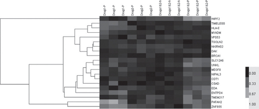
Figure 3.1 A heatmap visualization of a gene-by-subject expression datamatrix. Each row represents a gene and each column a subject. The characteristics of subjects are usually indicated above the columns. In this example, subjects were treated (P) or not treated (N) by Drugs 1 or 2. Three replicates were used for each treatment. The gene name is usually labeled to each row, on the right side of the matrix. A hierarchical tree is shown on the left side of the matrix to show the correlation of gene expression levels. Genes with similar expression profiles (in terms of high correlations) are presented closer to each other. Gene expression values are shown as gray scales. This image was generated by Cluster 3.0 and TreeView (Box 3.1)
Despite the similar appearance, RNA data matrices are distinct from DNA data matrices in light of the following aspects:
![]() Data associated to a subject are now represented by a column vector, rather than a row vector as in the DNA matrix.
Data associated to a subject are now represented by a column vector, rather than a row vector as in the DNA matrix.
![]() Each cell now contains a quantitative, floating point value representing the gene expression levels or their ratios, rather than the categorical data of genotypes.
Each cell now contains a quantitative, floating point value representing the gene expression levels or their ratios, rather than the categorical data of genotypes.
![]() The gene-by-sample matrix is commonly visualized using the heat maps, where the quantitative values are shown by a spectrum of colors.
The gene-by-sample matrix is commonly visualized using the heat maps, where the quantitative values are shown by a spectrum of colors.
![]() The genes are not required to be sorted according to the chromosomal positions; instead they are usually sorted by the similarity of gene expression patterns, so as to visualize the hidden modular activity in the heat map.
The genes are not required to be sorted according to the chromosomal positions; instead they are usually sorted by the similarity of gene expression patterns, so as to visualize the hidden modular activity in the heat map.
The sorting is done by methods such as hierarchical clustering or self- organizing maps (see Section 3.5.1 below on “similarity clustering”). In such cases, the hierarchical structure of genes may also be shown on the side of the heat map (Figure 3.1).
3.4.2 Contrast detection and the volcano plot
Contrast detection aims to find genes (probe sets) amongst all the assayed genes, which exhibit strong gene level contrast across distinct experimental or clinical conditions. In the presence of inevitable biological variation and noise, contrast detection needs to consider two issues:
1. The contrast is not likely to be false positive, a bottom line of an exploratory result.
2. The contrast should be large enough to bear biological functions.
Parametric statistical tests are commonly used to estimate the significance level, called P-values, of contrasting genes of two distinct experimental conditions. The design of the experiment can determine whether the samples are paired or non-paired. The paired samples are often two samples of the same subject at different time points (e.g. before or after medication) or from different tissues (i.e. tumor sample and adjacent healthy tissue). These samples can be compared by parametric, paired t-tests, which alleviate the cross subject heterogeneity and focus on the experimental contrast. However, the non-paired t-tests are used to assess the group average of experimental conditions.
The equation for non-paired two sample t-test (with unequal variance) is shown here to illustrate the principles of contrast detection (Rosner, 2006):
where g represents gene expression levels and c = {1,2} represents two distinct classes. n1 and n2 are the number of samples in the two groups, x1(g) and x2(g) represent the means of the two groups, and s1(g) and s2(g) represent the standard deviations of the measured data of the two groups respectively. The P-values, which represent the probability of false positive when there is no biological effect, can be derived based on t(g,c) and the degrees of freedom d:
A similar index of contrast is called the signal-to-noise ratio (SNR), also frequently used for microarray data analysis. The contrast of gene expressions is termed “signals”, while the standard deviations of the gene expression levels are termed “noise”. The equation is given as
Comparing the equations of SNR and t-tests, difference of mean expressions of the two groups are both presented in the numerator, and the standard deviations are both in the denominator. The idea is to select genes with large differences and small variations. SNR-based methods usually rely on the permutation test so as to generate an empirical null distribution. The significance level is then calculated based on the null distribution.
Often microarrays are used to explore expression patterns in more than two experimental or clinical conditions. In such cases, more elaborate methods than t-test or SNR are required. A variety of analysis strategy can be used, depending on the study purpose. First, the analysis of variance (ANOVA) test can test whether a gene has different expression profiles across various conditions. Second, several conditions may be regarded as the same and the samples aggregated as one group. For example, patients of Type 1 diabetes and rheumatoid arthritis may be pooled together as one group to be compared with healthy controls, based on the rationale that they both belong to autoimmune diseases (WTCCC, 2007). Third, if the clinical conditions are marked by levels of severity, then we may employ ordinal regression. For example, we may want to capture the molecular signature of cancer stages, or the five liver fibrosis stages F0 to F5 reflecting varying severity of the disease. Ordinal regression is an extension of logistic regression, which will be discussed in Chapter 4. Finally, a combination of the above strategies may be employed to form multiple constraints; for example, if the samples are of A, B and C conditions. We may select genes with a significant difference between A and B, as well as A and C. The multiple constraints aim to harvest genes to simultaneously fulfill all the constraints.
To adequately evaluate the contrasts, it is suggested that each group needs to have more than three biological samples. One major reason for the lower limit of sample size is to adequately quantify the variance (or standard deviation) of the expression levels.
The aforementioned parametric tests, such as t-tests and ANOVA, both assume the data are sampled from normal (i.e. Gaussian) distributions. In practice, the expression levels of genes often have skewed distributions across samples, many samples exhibit a relatively low value of expression levels toward zero, and a minority of samples demonstrate a very high value. The data distribution has a long tail toward the high value, clearly not a normal distribution. When the assumption of data normality is in question, the non-parametric methods can then be used (Mann and Whitney, 1947). The Mann–Whitney U tests are non-parametric alternatives to non-paired t-tests. The Wilcoxon signed-rank test is an alternative to paired t-tests. We can examine the data using methods such as the Lillifore test to check whether the data normality assumption is valid (Rosner, 2006).
Genes can then be ranked by their significance levels, which are the probability of false positive. In addition to the evaluation of significance levels, we also need to select the genes with larger expression level differences or folds across conditions, because they are more likely to bear salient biological functions. Scientists have selected genes based on fold changes, differences of means, SNR, P-values or their combinations. The combination of criteria can be illustrated by a volcano plot, which is a useful scatter plot for presenting the results of various contrast level analysis. It is particularly useful to show the combined gene selection criteria when multiple experimental conditions are assessed (Figure 3.2). The vertical axis usually indicates the negative log P-value. Genes with higher significance levels (i.e. smaller P-values) are shown in the top area of the plot. The horizontal axis can be used to represent the second criteria, such as the logged fold change, which is a common gauge of association used by many scientists. It can also represent the mean difference of the two conditions and the slope of a linear increase or decrease along the time axis or dose scale. An important consideration about the horizontal axis is to have a symmetrical scale for ups and downs. That is why the fold change value, the ratio of two expression levels, needs to be logged. The volcano plot is also useful for the presentation of genomic (DNA) variant association studies, where the vertical axis is still the logged P-value and the horizontal axis is the logged odds ratios.
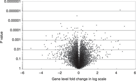
Figure 3.2 A typical volcano plot of a transcriptomics study. The x-axis shows the logged gene level fold change of case and control groups. The y-axis shows the negative log 10P value (This plot was generated by Excel.)
The different selection criteria will inevitably render different results. It has been an issue of debate whether the difference of means or fold change should be used for selection. Some prefer absolute differences (Tusher et al., 2001). MAQC prefer fold change rather than P-values, for reasons of consistency between studies.
Contrast level analysis can be calculated by spreadsheets and a variety of open sources, freeware (e.g. LIMMA and SAM (Box 3.1)) or commercial software available for microarray analysis, as well as statistical packages. Non-parametric tests can also be performed by a variety of statistical packages, such as SPSS.
3.4.3 Principal component analysis and PCA plots
Principal component analysis (PCA) and independent component analysis (ICA) are useful mathematical tools, which can generate plots to present the distribution of samples. In a transcriptomic data matrix, samples are characterized by levels of multiple assayed genes. These genes span a hyperspace of multiple orthogonal dimensions, one gene in each. Samples are pinpointed in the hyperspace based on the gene levels. For ease of comprehension, presentation of samples often requires dimension reduction methods. The PCA detects a 2-D or 3-D cross-section of the hyperspace, on to which the samples are projected (Figure 3.3).
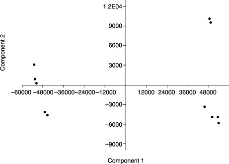
Figure 3.3 A 2-D plot by principal component analysis. Eleven samples are represented by the dots. The first and fourth quadrants represent samples of two different phenotypes. The dots in the second and third quadrants represent samples of one other phenotype. (This plot was generated by PAST software (Box 3.1).)
PCA and ICA are mathematical tools for the reduction of multivariate, high dimensional data. PCA and ICA are the top-down construction of representative vectors, and reduce high dimensional data into a presentation of fewer representative dimensions. Based on the data distribution in high dimensional space, PCA analysis extracts a series of principal components (linear transformed coordinates), where data in the first principal component has the largest variant. The second principal component is perpendicular (orthogonal) to the first principal component and has the second largest variant. The underlying assumption is that the coordinates with the large variants most saliently demonstrate the contrast between sample points, while the coordinates with smaller variants may be a source of noise, which should be ignored or suppressed. In the meantime, the correlation between two dimensions represents redundant information, which will not be presented. That is why this algorithm requires the following coordinates to be perpendicular (orthogonal) to previous coordinates. A PCA analysis can reduce the dataset of m dimension into n dimension, n<= m, by selecting the first n principal components.
However, ICA aims to decouple signals with distinct sources. This is also known as the blind source separation for solving the well-known cocktail party problem: detect each single conversation from a loud, noisy cocktail room. As opposed to PCA, the ICA does not utilize the orthogonal assumption that each representative component needs to be in the perpendicular. PCA and ICA can be performed in sequence. PCA is used first to extract the n principal components, then ICA is put in place to adjust the components so as to relax the orthogonal assumptions.
In transcriptomic data, samples are column vectors of m-dimensions, where m is the number of gene measurements. The samples are scattered in an m-dimensional vector space, where each gene is a dimension (or a coordinate). Each sample contributes a sample point (a dot) to the space. The sample vector is a vector linking the origin of the coordinate system toward the sample point.
3.4.4 Other global visualization methods
We have already seen the usefulness of the heat map for global visualization of gene level ups and downs under various experimental conditions (Figure 3.1). One additional useful class of plots is called 2-D scatter plots, which can be adapted for different purposes. Dots in a scatter plot represent a data point of a gene (or probe set). First, it can be used to show the dye intensity bias for two channel arrays, which is useful for platform level analysis. Second is the ratio intensity plot, also known as the M vs. A plot, where M is the fold change of two conditions. The fold change can be defined in one of several ways when more than two samples were measured, for example, the average of the paired fold, or fold change of the unpaired case and control samples averaged separately. The value is shown on the vertical axis. However, A represents the average gene expression level (e.g. the geometric means) shown on the horizontal axis.
3.5 Module level analysis
3.5.1 Similarity clustering – forming modules
Similarity clustering is an important step in the exploration and organization of expression profiles into modules. It can be used to group genes with similar expression profiles across samples, or samples with similar expression signatures across genes. Genes with similar expression profile are assumed to be co-expressed together by the same set of transcriptional factors, or for serving closely related cellular functions. The similarity of gene expressions makes it difficult to delineate which gene “causes” the expression of other genes. However, from another perspective, the similarity of gene expressions indicates that they can be analyzed together as a module to simplify the analysis. However, samples with similar expression profiles may represent the same clinical phenotypes, the same degree of external stimulation or drug treatment, or the same subtype of a heterogeneous disease. Similarities and differences are two sides of the same coin. For example, if the difference between two samples is defined as the Euclidean distance of their gene level vectors, then a smaller distance indicates a higher similarity.
This method has been used alone or in conjunction with contrast level analysis for drawing conclusions (Golub et al., 1999). If done alone, then the entire gene-by-sample matrix is clustered into modules, as long as the computational resource can process that much data. Modules of samples can represent subtypes of phenotypes such as cancer types, which are defined by all the gene levels of the transcriptomic data. If it is done before contrast level analysis, then the modules produced are further evaluated by their group contrasts, for example, the average of all genes across experimental conditions. If it is done after contrast level analysis, then the selected genes with significant differences are further grouped into modules, and each may represent an activated or suppressed cellular function. These methods can be used flexibly, depending on the purpose of the study. A heat map presentation usually is preceded by a similarity clustering for ease of comprehension and interpretation.
The clustering of samples by their similarity of expression vectors has been shown to be useful for disease sub-typing (Sarwal, 2003; Bhattacharjee et al., 2001). An unsupervised method was conducted, where the grouping was based purely on the gene expression signatures without the disease subtype of the samples. The disease subtype or clinical feature of each sample was known (by pathology tests), but temporarily undisclosed, so the analysis was done as if the subtype was unknown. The grouping result by unsupervised clustering was shown to be in good agreement with the known disease subtypes. Hence, it is certain that the molecular signature will be able to represent the macroscopic phenotype.
Clustering methods can be categorized as single layer or hierarchical methods, the latter being further divided into bottom-up or top-down approaches. The agglomerative hierarchical clustering method is a bottom-up process, where genes (or subjects) are progressively merged, based on the pairwise similarity between each pair of genes (subjects). Here the similarity of two vectors is often gauged by their pairwise Euclidean distance, Pearson’s or Spearman’s correlation. Hence, all genes (subjects) have equal opportunity to be merged with other genes. The Unweighted Pair Group Method with Arithmetic (UPGMA) mean method is an example of the bottom-up hierarchical clustering method. A tree-like hierarchical structure is progressively constructed, where the root of the tree represents a single large cluster containing all genes (subjects). Based on the tree, this cluster can be partitioned into several smaller, relatively homogeneous clusters, in the sense that the similarity between the cluster members is relatively lower. As we trace from the root further down, more cluster will be generated, and each cluster will be more homogeneous. Thus the number of clusters is adjustable by the investigator for interpretation of the data. Each cluster can be seen as a module, as the genes (subjects) within a cluster share a similar expression profile, implying their similar cellular role (for a gene module) or disease subtype (for a sample module). The Cluster 3.0 software (Eisen et al., 1998; de Hoon et al., 2004) is a widely used, public domain software for hierarchical clustering (Box 3.1). Its results can be conveniently loaded into the visualization software TreeView (Saldanha, 2004) (Box 3.1).
The single-layer clustering methods are exemplified by the k-means clustering and self-organizing map (Chaussabel et al., 2008; Golub et al., 1999). K-means clustering is an iterative process where the members associated to the clusters, and the cluster centroids, are progressively updated until a stable state is reached. This requires the vector to be standardized to a zero mean and unit variance. However, this method requires the number of clusters to be determined before analysis. Global clustering methods are useful for time-course analysis where genes co- expressed in time result in similar time-course profiles, which are then grouped together.
It is also commonplace to have arrays assayed at different time points. This type of experiment often requires clustering of genes of a similar time course profile. In such cases, various clustering techniques can be used. For example, k-means clustering has been employed in time course data of neutrophil activation experiments (Kotz et al., 2010).
We can add some twists based on the same concept of grouping of genes into modules to extend the range of applications. Instead of grouping directly, based on the similarity of expression patterns, we can also base on the frequency of oscillatory gene expression, which may have different phases (Kim et al., 2008). Genes with the same frequency but with different time lags may actually serve the same periodic cellular role.
3.5.2 Functional annotations of activated biological modules
Contrast level analysis renders a focused set of genes or probe sets of interest, which show stronger associations with the contrast of experimental conditions. Once the subset of genes is identified, the next step is to explore the functional significances of the genes individually. The first step is to extract preliminary annotations of each gene in the subset via microarray vendor websites (i.e. Affymetrix NetAffx website), or other online databases (i.e. DAVID website (Box 3.1)). Annotations obtained in this way usually include a fairly general description of the gene, such as its gene ID, symbol, sequence ID, location in the genome, and a few lines of summary of functions. This information is often too preliminary to conclude the experiment. One solution is to query a multiple database so as to produce a tailor-made annotation for a particular study.
Preliminary annotation can be quickly obtained; however, the real challenge lies in the module-level annotation to partition, filter or organize the short-list of genes into functional modules so as to account for the total experiment. This is probably the most challenging and critical step before forming a theory and drawing a conclusion.
Enrichment analysis is a frequently-used approach for functional annotations. This is done by matching the focused set of genes to all known pathway modules (e.g. the extrinsic apoptosis pathway, the renin- angiotensin pathway, etc.) or gene ontology modules with respect to molecular functions, cellular components or biological processes. The analysis detects modules with matches of genes significantly higher or lower than expected values, showing that the focused set of genes is enriched or deprived in the module of interest. The significance is often assessed by the hypergeometric test. Assuming the total number of genes in the human genome is N and those in that module of interest is m, and assuming the number of genes in the focused set is n and the number of matches is k, then the probability of k in the hypergeometric distribution is:
An up- and down-regulated subset of genes can be submitted for enrichment analysis together or separately. It is often easier to do them separately.
The underlying assumption behind the enrichment analysis-based annotation is that functions of active modules (either boosted or suppressed) may manifest by the distribution of constituent genes. Hence, a module enriched or deprived with the genes in a pathway suggests that the pathway may play a salient role in the topic under investigation. Gene vs. module matching offers a type of domain knowledge filter to sift important genes segregated into modules from a background of noise. However, this assumption is not always true. In practice, the focused set of genes often scatter in different directions. Those genes not enriched in a module are left unexplained, despite the fact that they may actually play key roles. They could either work alone, or synergistically, in a way we still do not understand and thus are not enriched in any particular pathway (yet). This is one major drawback of the use of enrichment analysis at the present time.
Therefore, the success of enrichment analysis highly depends on the accuracy and completeness of the genes in the pathway database. As the pathway information is still incomplete and new knowledge is accumulating fast, using software with the most recent pathway information will hopefully improve the quality of functional annotation. In addition, pathway usually contain a smaller number of genes than a biological process, and the former may offer high specificity but lack sensitivity. This suggests that we should conduct functional annotations using both types of module so as to better understand the result.
A variety of online software tools for enrichment analysis are currently available. The PANTHER (Protein ANalysis THrough Evolutionary Relationships) Classification System is a valuable functional annotation website, which offers a global presentation for the comparison of two focused sets of genes, an ideal feature for presenting both the up- and down-regulated genes (Thomas et al., 2003). The GOEAST (Gene Ontology Enrichment Analysis Software Toolkit) website provides a convenient tree-structure presentation (Zheng and Wang, 2010) (Box 3.1). The DAVID site by NIH is very useful as it provides an integrated analysis of gene ontology categories and pathways. In addition, many gene ontology packages are available as plug-i ns to the Cytoscape software, a graph- centered software platform (Box 5.1). These packages are excellent for building network presentations of gene ontology terms. GoMiner and GenMapp are useful software for annotation analysis.
Metacore is a commercial software package for module level functional annotations in the pathway or gene ontology analysis. One special feature of the software is the ability to build a set of genes into a network. Genes are linked if there is a literature reference connecting the two genes. Needless to say, this relies on the literature mining done by the company.
3.5.3 Gene expression matching
One other approach of module level analysis is to match the focused gene of one experiment directly to another experiment. A good match indicates that the underlying mechanisms behind the two experiments are similar. This is actually engineering style thinking to regard a complex, isolated system (in this case, an experimental perturbation of genome-wide RNA levels) as a “black box”, and then try to characterize the system by inputs and outputs. The same outputs indicate the same inputs. This idea also applies to “opposite” gene expression alteration pattern (a reverse of up and down), which suggests an antagonizing effect. If a drug produces an opposite expression pattern of a disease, then the drug may be a good therapeutic agent for the disease. As a result, the gene expression pattern becomes a common intermediate across different experiments.
To put this concept into practice, a reference dataset needs to be established first. Lamb et al. (2006) conducted a series of in vitro microarray experiments on cell lines stimulated by various currently used drugs, providing the reference dataset for gene expression matching. Microarray experiments were conducted before and after drug stimulation. The reference database is called the Connectivity Map (Box 3.1).
A focused set of genes can be submitted to the Connectivity Map server. The direct and opposite matches indicate the clues of mechanisms behind the gene expression alterations of the focused set of genes. The server employs the Kolmogorov–Smirnov statistic-like scores to handle the matches. First, up- and down-regulated genes are matched separately, then combined together for ranking of similarities. The Kolmogorov- Smirnov test is a non-parametric method to test the similarity of distribution functions. The server also uses permutation methods to calculate significance levels of matches (i.e. P-values).
3.5.4 Gene Set Enrichment Analysis
The Gene Set Enrichment Analysis (GSEA) algorithm and software, offered by the Broad Institute, represents another class of module level analysis (Subramanian et al., 2005; Mootha et al., 2003). The goal is to analyze the focused set of genes to see whether they are the leading perturbed genes amongst all the genes. P-values are derived from an empirical distribution of permutations of the class labels.
3.6 Systems level analysis for causal inference
Systems level analysis refers to the joint analysis of multiple systems, such as the genomics and transcriptomics. Coherent evidence derived from different systems can enhance the evidence level and the confidence. A joint analysis involves both integrators and filters, an analogy drawn from common signal processing devices seen in digital circuits (Ideker et al., 2011). Contrast and module level analysis can be seen as filters to remove biologically irrelevant noise from true signals. Now we will explore the integration of multiple datasets.
Each individual discovery of association between germline, somatic DNA variants or RNA expressions and a diseased state is a milestone. Often the association is based on the grounds of statistical associations rather than mechanistic explanations. Not every genetic variant associated to disease reflects the cause of the disease, because many adjacent DNA variants are correlated with each other, known as the linkage disequilibrium phenomenon (Chapter 2). In such cases it is difficult to distinguish the real causative SNP from the adjacent, statistically associated but not causative SNPs. Similarly, not every gene expression associated with the disease reflects the cause of the disease, because the expressions of multiple genes are usually correlated to each other due to their intricate regulations, which might not be directly responsible for the trait.
Once a germline or somatic variant is statistically confirmed to be associated to a disease, the underlying mechanical cause may be hypothesized, depending on the location of the variant in relation to a gene:
1. If the variant is in the coding region of the exon, and the different alleles code for different amino acids (called a non-synonymous variant), then the amino acid variant may be responsible for altered protein structure or function efficiency, which may be the cause of the disease. This hypothesis can be further validated by protein assays.
2. If the variant is in the coding region of the exon, but different alleles do not code for different amino acids (called a synonymous variant), then it may be hypothesized that this variant will change translation efficiency.
3. If the variant is in the exonic UTR, such as 3’UTRs and 5’UTRs, then it may be postulated to change RNA regulations.
4. If the variant is in the intronic region, then it may be postulated to cause RNA splicing patterns. This will further cause protein level change. This hypothesis can be substantiated by checking the relationship between variant and mRNA alternative splicing forms.
5. If the variant is around the promoter and transcription element region, then this variant may be implicated on transcriptional efficiency, therefore affecting the RNA (and then protein) expression pattern.
Each hypothesis can indicate subsequent designs of validation studies to illustrate the mechanical cause (Peer and Hacohen, 2011). For scenarios 3, 4 and 5, a joint analysis of genomics and transcriptomics is justified. Gene expression has been shown to correlate with GWAS studies under certain conditions (Gorlov, 2010). A causal, mechanistic relationship between genes and phenotypes under scenarios 3 to 5 includes three criteria:
With the transcriptomics platforms such as exon arrays or expression arrays in place, an integrated study design and concurrent analysis is motivated (Schadt et al., 2005). Criteria B and C are first examined individually by genome-wide contrast level analysis. DNA and RNA are preferably measured in the same samples, but using different samples is also plausible. RNA sample sources particularly need to be considered carefully, as the expression of many genes is restricted to certain cell or tissue types or upon a particular stimulation. If the hypothesis is related to gene activity on, for example, tumor cells, then a tumor specimen may be required.
There are three strategies to complete constructs A, B and C:
![]() Strategy 1: find the subset of genes that have both DNA variants and RNA expressions associated to the phenotype (i.e. constructs B and C established). Check for association between DNA variants and RNA expressions (construct A).
Strategy 1: find the subset of genes that have both DNA variants and RNA expressions associated to the phenotype (i.e. constructs B and C established). Check for association between DNA variants and RNA expressions (construct A).
![]() Strategy 2: similar to strategy 1 but in a more relaxed way. Genes adjacent to associated DNA variants are included in the analysis. Similarly, genes in the upstream or downstream pathways of associated RNA expressions are considered. The subset of genes is then calculated by the intersection of the augmented gene sets.
Strategy 2: similar to strategy 1 but in a more relaxed way. Genes adjacent to associated DNA variants are included in the analysis. Similarly, genes in the upstream or downstream pathways of associated RNA expressions are considered. The subset of genes is then calculated by the intersection of the augmented gene sets.
![]() Strategy 3: use the conditional probability to depict the causal model as
Strategy 3: use the conditional probability to depict the causal model as
where a DNA variant on a locus is denoted as L, the clinical phenotype is denoted as C, and the RNA expression is denoted as R (Schadt et al., 2005). The probability of clinical phenotype is conditioned by the DNA variant and RNA expression.
The construct A in strategy 3 is denoted as PR(LlR), which can be established by the analysis of quantitative trait locus (QTL), used to refer to the connection between the DNA variants to quantitative traits, such as gene expressions, or quantitative diseased states, such as elevated fasting glucose levels and HBa1C measurements in diabetic patients. The expression QTL (eQTL) is particularly used to refer QTL analysis correlating DNA variants to its corresponding RNA expressions.
Naturally, the analysis can be extended to protein level analysis to establish a more solid mechanistic explanation such as:
where the protein expression is denoted by P.
Despite the analysis that causal inference can eliminate several false positives, and increase evidence level, it remains a difficult task to find driver somatic mutations in cancer studies. This is because cancer has a complex progressive development. So many somatic mutations occur during the progress. The drivers are assumed to be critical in the process. The passengers could also demonstrate a mechanistic link of constructs A, and weakly B and C, and they may not play essential roles.
3.7 RNA secondary structure analysis
It is becoming clear that RNA molecules do not merely serve as passive information templates, but also carry important enzymatic and regulatory functions. RNA transcripts have secondary structures that are related to the half life, the stability, the functions and the interactions with other macromolecules. Computational analysis of RNA secondary structure is thus important for characterizing its roles. RNA secondary structures of one or two molecules can be predicted using the standalone Vienna RNA package (Hofacker et al., 1994; Hofacker, 2003). This is mainly based on the thermodynamic properties of base pairing, the net energy of which can be estimated as kilocalories per mole of RNA (kcal/mol).
3.8 Case studies
3.8.1 Molecular signature for allograft rejection after renal transplantation
Kidney transplantation is one of the few therapeutic choices currently available for patients with end-stage renal diseases. For such a therapy, recipients’ acute immune rejection to allografts has been the major cause of failure. The detailed molecular mechanism of allograft rejection is still elusive. Furthermore, the histology of biopsy samples does not offer sufficient information for prediction of allograft rejection (Sarwal et al., 2003). The exploration of allograft transcriptomes may shed light on this critical yet unclear mechanism.
Sarwal et al. (2003) reported a gene expression study on biopsy specimens of patients with acute rejection after renal transplantation. A total of 67 biopsy samples, from 59 children and young adults, and 8 donors, were examined. Among them, 9 had allograft loss (which means treatment failure) due to intolerable host rejection. A complementary DNA (cDNA) microarray was used for the exploration mechanism, where the expression levels of 14,220 genes were measured using 28,032 probes. All of the samples showed no signs of lymphoproliferative disorder by histological examination which, therefore, cannot distinguish patients with elevated risks of allograft loss from the others.
The authors conducted a two-stage exploration analysis. The first stage was a grouping of samples using the bottom-up hierarchical clustering method. Gene expression levels were first normalized as folds with respect to the gene-specific mean expressions across all samples. This ensured the mean values of every single gene to be 1, therefore genes with low expression levels could also contribute to the grouping of samples. The similarity between pairs of samples was then quantified by Pearson correlation coefficients. The clustering was done as if the clinical status of the subjects was unknown, that is, an unsupervised method. The samples were grouped by the algorithm into four major clusters:
A later called the allograft rejection 1;
B comprising two groups, allograft rejection 2 and toxic drug effects and infection;
C also comprising two groups, allograft rejection 3 and chronic allograft nephropathy; and
An interactive heat map is presented online on the authors’ website at Stanford University, using the GeneExplorer software to show the distinct characteristics of the four groups.
Based on the clusters defined in the first stage, the authors then examined the gene expression contrasts using the SAM method. They identified a focused set of 385 genes over-expressed in the allograft rejection 1 group compared with other subtypes. A functional annotation (based on enrichment analysis using the hypergeometric test) showed that the T cell related genes are particularly enriched in the over-expressed set of genes. This is consistent with the known significant role of T cell infiltration in the rejection mechanism. What is unexpected is the appearance of several B cell related genes, particularly the CD20, on the focused gene set. The roles of CD20 and B cell infiltration are the major novel discovery in kidney allograft rejection. All the methods used (hierarchical clustering, SAM, enrichment analysis) have been detailed in previous sections.
To confirm the findings of RNA level microarray analysis, a monoclonal antibody of CD20 was employed for the immunostaining on 20 biopsy samples, a subset of the original study cohort. It was found that 8 out of 9 CD20 positive samples belonged to patients with allograft loss or incomplete functional recovery. In contrast, only 1 out of 11 CD20 negative samples was associated to such a poor condition (P < 0.001). The protein level results further confirmed the findings on the RNA level exploration, a step toward clinical use. The corresponding Positive Predictive value was 88.9% and Negative Predictive Value was 90.9 (see Chapter 6 for definition). This is an excellent performance, as long as it can be validated in independent cohorts with larger sample sizes. In the future, immunostaining of CD20 might improve the clinical evaluation of the risks of allograft loss.
3.8.2 Molecular model for follicular lymphoma prognosis
Follicular lymphoma is a heterogeneous disease with patients’ prognosis and life expectancy varying greatly, ranging between 1 to 20 years (Dave et al., 2004). The disease in some patients manifested a long-term dormant state, while in others it manifested a rapid progression. Causes for the variability remain a mystery. Thus, personally optimized treatment of follicular lymphoma has not yet been established. Exploration of the molecular signature may help to illuminate the disease mechanism, which might lead toward the prediction of prognosis and therefore the optimal personalized treatment.
Dave et al. (2004) collected 191 pretreatment tumor biopsy specimens and assigned them evenly into the training group (n = 95) and the validation group (n = 96). Gene expressions on these specimens were assayed using Affymetrix U133A and U133B microarrays. These subjects then received a variety of treatments or were followed without treatment. Overall survival was observed. An association between genes and overall survival time was evaluated in the training group by the Cox proportional hazard model. The gene by subject matrix was then visualized as two heat maps, where genes positively and negatively associated to survival time were separately presented. The gene expression levels were adjusted to folds with respect to the gene-specific medians across all samples. This ensured the median of every single gene to be 1.
A hierarchical clustering was then performed on genes. Ten gene clusters were identified where genes within a cluster had similar expression profiles across subjects, with Pearson correlation coefficient r > 0.5 between each other. The expression levels of genes in a cluster were then averaged to serve as a representative value for that cluster. In this way, the data were boiled down to a 10 variable signature per subject. An exhaustive enumeration of all pairwise combinations was performed, and a combination of two variables, called the immune response 1 and 2 respectively, had the strongest prediction performance of overall survival (p < 0.001 in both the training and validation groups). Elevated immune response 1 was associated to longer overall survival, while elevated immune response 2 was associated to shorter survival. An attempt was made to add one more variable to the two-variable signature, achieving a prediction p < 0.001 in the training cohort and p = 0.003 in the validation cohort. However, the third variable does not seem to contribute to the total prediction performance and so was dropped from the model.
The patients were then sub-grouped by the two-variable model into four quarters. The corresponding Keplan–Meier curves were used for visualization. The survival medians of the subgroups were 13.6, 11.1, 10.8 and 3.9 years, respectively. The last quarter of patients deserve specialized attention, as they represented a high-risk group with shorter survival.
3.8.3 Molecular similarity between stem and cancer cells
The cancer stem cell model is an insightful hypothesis of cancer initiation, progression and resistance to chemotherapy, which has a profound impact on cancer biology and treatment strategies. This model suggests that a class of stem cell like cancer cells are at the top of the hierarchy of heterogeneous cancer tissue. These cancer stem cells are responsible for driving the progression and, unlike other cancer cells, cannot be easily eliminated by chemotherapeutic agents. Cancers have been known to exhibit characteristics of reverse differentiation, such as the known Epithelial Mesenchymal Transition frequently observed in the metastatic stage of cancer progression. Gene expressions of de-differentiation markers have actually been used for the clinical staging of cancer.
Ben-Porath et al. (2008) conducted an analysis of transcriptomics of tumor specimens to explore the similar molecular signature between stem and cancer cells. The analysis is a sophisticated, two-pass enrichment analysis of gene expression data, with gene expression similarity between cancer and stem cells, where the genes are grouped into modules to facilitate the analysis. It combines enrichment analysis mentioned earlier with the grouping of related genes, clinical features and sample types. First, the gene signature of the human embryonic stem cell (hES) is defined based on previous studies. For example, genes over-expressed in more than five stem cell profiling studies were defined as a hES gene set. Second, genes over-expressed in individual cancer specimens were evaluated to see whether they were enriched in the pre-defined gene sets. In other words, they mapped real array data of cancer into stem cell classes. Third, they further conducted a second pass of enrichment calculation to see whether samples of the same type had similar enrichment patterns. This is a way to collapse a large gene-by-sample data matrix into a smaller, biologically more interpretable “gene class” by “sample group” matrix. They concluded that cancer cells do over-express genes that are normally associated with stem cells.
There are two important features for this type of analysis. First, enrichment analysis is used where genes are represented in either the “on” state (e.g. gene is over-expressed) or “off” state (e.g. gene is under-expressed). The quantitative measures of gene expressions need to be thresholded, either in absolute quantities or fold changes, to get either an “on” or “off” state. The genes with “on” states are then mapped to the gene classes of interest to see whether they are enriched. Second, the enrichment statistics are based on hypergeometric tests. The collection of sample types will determine the result of enrichment analysis.
3.9 Take home messages
![]() RNA molecules carry important regulatory and enzymatic functions, in addition to serving as templates for protein synthesis.
RNA molecules carry important regulatory and enzymatic functions, in addition to serving as templates for protein synthesis.
![]() Microarrays and NGS are two important transcriptomic platforms, each with its strengths.
Microarrays and NGS are two important transcriptomic platforms, each with its strengths.
![]() Contrast level analysis is mostly done by statistical tests.
Contrast level analysis is mostly done by statistical tests.
![]() Module level, enrichment analysis can be done by gene ontology (GOEAST), Connectivity Map analysis, DAVID, GSEA, Enrichnet and PANTHER.
Module level, enrichment analysis can be done by gene ontology (GOEAST), Connectivity Map analysis, DAVID, GSEA, Enrichnet and PANTHER.
![]() Visualization methods such as the volcano plots can be used to present and analyze the results of multiple contrast criteria, particularly when the transcriptomic dataset represents more than two phenotypes.
Visualization methods such as the volcano plots can be used to present and analyze the results of multiple contrast criteria, particularly when the transcriptomic dataset represents more than two phenotypes.
3.10 References
Ben-Porath, I., Thomson, M.W., Carey, V.J., Ge, R., Bell, G.W., et al. An embryonic stem cell-like gene expression signature in poorly differentiated aggressive human tumors. Nat Genet. 2008; 40(5):499–507.
Bhattacharjee, A., Richards, W.G., Staunton, J., Li, C., Monti, S., et al. Classification of human lung carcinomas by mRNA expression profiling reveals distinct adenocarcinoma subclasses. Proc. Natl. Acad. Sci. USA. 2001; 98:13790–13795.
Bolstad, B.M., Irizarry, R.A., Astrand, M., et al. A comparison of normalization methods for high density oligonucleotide array data based on bias and variance. Bioinformatics. 2003; 19(2):185–193.
Carthew, R.W., Sontheimer, E.J. Origins and mechanisms of miRNAs and siRNAs. Cell. 2009; 136(4):642–655.
Cech, T.R. The RNA Worlds in Context. Source: Department of Chemistry and Biochemistry. University of Colorado, Boulder, Colorado, 2011., doi: 10.1101/cshperspect.a006742. [80309–0215. Cold Spring Harb. Perspect. Biol. 16 February. p. ii: cshperspect.a006742v1].
Chaussabel, D., Quinn, C., Shen, J. A modular analysis framework for blood genomics studies: Application to systemic lupus erythematosus. Immunity. 2008; 29(1):150–164.
Dave, S.S., Wright, G., Tan, B., Rosenwald, A., et al. Prediction of survival in follicular lymphoma based on molecular features of tumor-infiltrating immune cells. N. Engl. J. Med. 2004; 351(21):2159–2169.
de Hoon, M.J., Imoto, S., Nolan, J., et al. Open source clustering software. Bioinformatics. 2004; 20(9):1453–1454.
Dysvik, B., Jonassen, I. J-Express: Exploring gene expression data using JAVA. Bioinformatics, 2001. 2001; 17(4):369–370.
Eddy, S.R. Non-coding RNA genes and the modern RNA world. Nat. Rev. Genet. 2001; 2(12):919–929.
Eisen, M.B., Spellman, P.T., Brown, P.O., Botstein, D. Cluster analysis and display of genome-wide expression patterns. Proc. Natl. Acad. Sci. USA. 1998; 95:14863–14868.
Gamsiz, E.D., Ouyang, Q., Schmidt, M., et al. Genome-wide transcriptome analysis in murine neural retina using high-throughput RNA sequencing. Genomics. 2012; 99(1):44–51.
Geiss, G.K., Bumgarner, R.E., Birditt, B., Dahl, T., Dowidar, N., et al. Direct multiplexed measurement of gene expression with color-coded probe pairs. Nat. Biotechnol. 2008; 26(3):317–325.
Glaab, E., Baudot, A., Krasnogor, N., Schneider, R., Valencia, A. EnrichNet: Network-based gene set enrichment analysis. Bioinformatics. 2012; 28(18):i451–i457.
Golub, T.R., Slonim, D.K., Tamayo, P., Huard, C., Gaasenbeek, M., et al. Molecular classification of cancer: Class discovery and class prediction by gene expression monitoring. Science. 1999; 286:531–537.
Gorlov, I.P. GWAS Meets Microarray: Are the Results of Genome-Wide Association Studies and Gene-Expression Profiling Consistent? Prostate Cancer as an Example. PLOS one. 2010.
Hofacker, I.L., et al. Fast folding and comparison of RNA secondary structures. Monatsh. Chem. 1994; 125:167–188.
Hofacker, I.L. Vienna RNA secondary structure server. Nucleic Acids Res. 2003; 31(13):3429–3431.
IHGSC. Finishing the euchromatic sequence of the human genome. Nature. 2004; 431:931–945.
Ideker, T., Dutkowski, J., Leroy Hood, L. Boosting signal-to-noise in complex biology: Prior knowledge is power. Cell. 2011; 144:860–863.
Irizarry, R.A., Bolstad, B.M., Collin, F., et al. Summaries of Affymetrix GeneChip probe level data. Nucleic Acids Res. 2003; 31(4):e15.
Irizarry, R.A., Hobbs, B., Collin, F., et al. Exploration, normalization, and summaries of high density oligonucleotide array probe level data. Biostatistics. 2003; 4(2):249–264.
Kerr, K.F. Extended analysis of benchmark datasets for Agilent two-color microarrays. BMC Bioinformatics. 2007; 8:371.
Kim, C.S., Riikonen, P., Salakoski, T. Detecting biological associations between genes based on the theory of phase synchronization. Biosystems. 2008; 92(2):99–113.
Kotz, K.T., Xiao, W., Miller-Graziano, C. Clinical microfluidics for neutrophil genomics and proteomics. Nat Med. 2010; 16(9):1042–1047.
Lamb, J., Crawford, E.D., Peck, D. The Connectivity Map: Using geneexpression signatures to connect small molecules, genes, and disease. Science. 2006; 313(5795):1929–1935.
Mann, H.B., Whitney, D.R. On a test of whether one or to random variables is stochastically larger than the other. Annals of Math. Stat. 1947; 18:50–60.
MAQC. The microarray quality control (MAQC) project shows inter- and intraplatform reproducibility of gene expression measurements. Nat Biotechnol. 2006; 24:1151–1161.
Mootha, V.K., Lindgren, C.M., Eriksson, K.F., et al. PGC-1alpha-responsive genes involved in oxidative phosphorylation are coordinately downregulated in human diabetes. Nat Genet. 2003; 34(3):267–273.
Nagano, T., Fraser, P. No-nonsense functions for long non-coding RNAs. Cell. 2011; 145:178–181.
Okazaki, Y., et al. Analysis of the mouse transcriptome based on functional annotation of 60,770 full-length cDNAs. Nature. 2002; 420(6915):563–573.
Patterson, T.A., Lobenhofer, E.K., Fulmer-Smentek, S.B., Collins, P.J., Chu, T., et al. Performance comparison of one-color and two-color platforms within the Microarray Quality Control (MAQC) project, 2006.
Peer, D., Hacohen, N. Principles and strategies for developing network models in cancer. Cell. 2011; 144:864–873.
Qin, L., et al. Empirical evaluation of data transformations and ranking statistics for microarray analysis. Nucleic Acids Res. 2004; 32:5471–5479.
Rosner, B. Fundamentals of Biostatistics. USA: Thomson; 2006.
Saldanha, A.J. JAVA Treeview: Extensible visualization of microarray data. Bioinformatics. 2004; 20(17):3246–3248.
Sarwal, M. Molecular heterogeneity in acute renal allograft rejection identified by DNA microarray profiling, New Eng. J. Med. 2003; 349:125–138.
Schadt, E.E., et al. An integrative genomics approach to infer causal associations between gene expression and disease. Nat Genet. 2005; 37:710–717.
Subramanian, A., Tamayo, P., Mootha, V.K., et al. Gene set enrichment analysis: A knowledge-based approach for interpreting genome-wide expression profiles. Proc. Natl. Acad. Sci. USA. 2005; 102(43):15545–15550.
Thomas, P.D., Kejariwal, A., Campbell, M.J., et al. PANTHER: a browsable database of gene products organized by biological function, using curated protein family and subfamily classification. Nucleic Acids Res. 2003; 31(1):334–341.
Tusher, V.G., Tibshiranim, R., Chu, G. Significance analysis of microarrays applied to ionizing radiation response. Proc. Natl. Acad. Sci. USA. 2001; 98:5116–5121.
WTCCC. Genome-wide association study of 14,000 cases of 7 common diseases and 3000 shared controls. Nature. 2007; 447:661–678.
Zheng, Q., Wang, X.J. GOEAST: A web-based software toolkit for gene ontology enrichment analysis. Nucleic Acids Res. 2008; 36:358–363.