
Chapter 7. Serving Models and Architectures
As we think about how recommendation systems utilize the available data to learn, and eventually serve recommendations, it’s crucial to describe how the pieces fit together. The combination of the data flow, and the jointly available data for learning, is called the architecture. More formally, the architecture is the connections and interactions of the system or network of services – for data applications it also includes the available features and objective functions for each sub-system. Defining the architecture typically involves identifying components or individual services, defining the relationships and dependencies between those components, and specifying the protocols or interfaces through which they will communicate.
In this chapter, we’ll spell out some of the most popular and important architectures for recommendation systems.
Architectures by Recommendation Structure
We have returned several times to the concept of Collector, Ranker, Server, and we’ve seen that they may be regarded via two paradigms: the online and the offline modes. Further, we’ve seen how many of the components in the last chapter on data processing satisfy some of the core requirements of these functions.
In designing large systems like these, there are a number of architectural considerations; now we will demonstrate how these concept are adapted based on the type of recommendation system you are building. In this chapter, we compare a mostly standard item-to-user recommendation system, a query-based recommendation system, contextual recommendations, and sequence-based recommendations.
Item-to-User recommendations
We’ll start by describing the architecture of the system we’ve been building in the book thus far. As proposed in Chapter 4, we built the collector offline to ingest and process our recommendations. We utilize representations to encode relationships between items, users, or user-item pairs. The online collector takes the request, usually in the form of a user-id, and finds a neighborhood of items in this representation space to pass along to the ranker. Those items are filtered when appropriate and sent for scoring. The offline ranker learns the relevant features for scoring and ranking, training on the historical data. It then uses this model and, in some cases, item features as well for inference. In the case of recommendation systems this inference computes the scores associated to each item in the set of potential recs. We usually sort by this score Part III. Finally, we integrate a final round of ordering based on some business logic Chapter 14. This last step is part of the serving where we impose things like test-criteria or recommendation diversity requirements.

Figure 7-1. This image by Karl Higley and Even Oldridge is an excellent overview of the Retrieval, Ranking, Serving Structure, although they instead use four stages and slightly different terminology. In this text, we combine Filtering into Retrieval. (used with permission)
Query-based recommendations
To start off our process, we want to make a query. The most obvious example of a query is a text query like in text-based search engines; however, queries may be more general! For example you may wish to allow search-by-image, or search-by-tag. Note that an important type of query-based recommender is where the query is implicit; i.e. where the user is providing a search query via UI choices, or by behaviors. While these systems are quite similar in overall structure to the item-to-user systems, let’s discover how to modify them to fit our use-case.
We wish to integrate more context about the query into the first step of the request. Note that we don’t want to throw out the user-item matching components of this system – even though the user is performing a search, there’s utility in personalizing the recommendations based on their taste. Instead we need to utilize the query in addition; later we will discuss various technical strategies, but a simple summary for now is to also generate an embedding for the query! Note that the query is like an item or a user, but sufficiently different. Some strategies might include similarity between the query and items, or co-occurrence of the query and items. Either way, we now have a query-representation and user-representation, and we want to utilize both for our recommendation. One simple strategy here is to use the query representation for retrieval, but during the scoring, score via both query-item and user-item, combining them via a multi-objective loss. Another strategy is to use the user for retrieval, and then the query for filtering.
Different embeddings
Unfortunately, while we’d love the same embedding space (for nearest neighbors lookup) to work well for our queries and our documents (items, etc.) this is often not the case. The most simple example is something like like asking questions and hoping to find relevant Wikipedia articles. This problem is often referred to as the queries being “out of distribution” from the documents.
Wikipedia articles are written in a declarative informative article style, whereas questions one might ask are often brief, and casual. If you were to use an embedding model that is focused on capturing semantic meaning, you’d naively expect that the queries to be located in significantly different subspaces than the articles. This means that your distance computations will be effected. This is often not a huge problem because you retrieve via relative distances, and you can hope that the shared subspaces are enough to provide a good retrieval. However, it can be hard to predict when these perform poorly.
The best practice is to carefully examine the embeddings on common queries, and on target results. These problems can be especially bad on implicit queries like a series of actions taken at a particular time of day to look up food recommendations. In this case, we expect the queries to be wildly different than the documents.
Context-based recommendations
A context is actually quite similar to a query, but tends to be more obviously feature based and frequently less similar to the items/users distributions.. Context is usually the term use to represent some exogenous features to the system, that may have an effect on the system, i.e. auxiliary information such as time, weather, location, and more. The ways in which it is similar to query-based recommendation are that it’s an additional signal that the system needs to consider during recommendation, but more often than not: query should often dominate the signal for recommendation, whereas context should not.
Let’s take a simple example: when ordering food. A query for a food-delivery recommendation system would look like Mexican food; an extremely important signal from the user looking for burritos or quesadilla of how the recs should look. A context for a food-delivery recommendation system would look like it’s almost lunch time. This is an useful signal, but may not out-weigh user-personalization. It’s hard to put hard and fast rules on this weighting, so usually we don’t, and instead learn parameters via experimentation.
How context features fit into the architecture is very similar to queries, via learned weightings as part of the objective function. Your model will learn a representation between context features and items, and add that affinity into the rest of the pipeline. Again you can make use of this early in the retrieval, later in the ranking, or even during the serving step.
Sequence-based recommendations
Sequence based recommendations build on context-based recommendations, but with a specific type of context. Sequential recommendations use the idea that the recent items the user has been exposed to should have a significant influence on the recommendations. A common example here is a music streaming service, where the last few songs that have been played can significantly inform what the user might want to hear next. To ensure this auto-regressive, or sequentially predictive, set of features has an influence on recommendations, we can treat each item in the sequence as a weighted context for the recommendation.
Usually, the item-item representation similarities are weighted to provide a collection of recommendations and various strategies are used for combining these. In this case, we normally expect the user to be of high importance in the recommendations but the sequence is also of high importance. One simple model is to think of the sequence of items like a sequence of tokens, and form a single embedding for that sequence – like in NLP applications. This embedding can be used as the context in a context-based recommendation architecture.
Naive sequence embeddings
The combinatorics of one-embedding-per-sequence explodes in cardinality; the number of potential items in each sequential slot is very large, and each item in the sequence multiplies those possibilities together. Image for example 5 word sequences, where the number of possibility for each item is close to the size of the English lexicon, and thus it would be that size to the 5th power. We provide some simple strategies for dealing with this in Chapter 17.
Why bother with extra features
Sometimes it is useful to step back and ask if a new technology is actually worth caring about. So far in this section we’ve introduce four new paradigms for how to think about a recommender problem. That level of detail may seem surprising and potentially even unnecessary.
One of the core reasons that things like context and query based recommendations become relevant is to deal with some of the issues mentioned before around sparsity and cold starting. Sparsity makes things that aren’t cold seem cold via the learner’s under-exposure to them, but true cold starting also exists due to new items being added to catalogs with high frequency in most applications. We will address cold-starting in detail, but for now, suffice to say that one strategy for warm starting is to use other features which are available even in this regime.
In applications of machine learning that are explicitly feature based, we rarely battle the cold-start problem to such a degree, because at inference time we’re confident that the model parameters useful for prediction are well aligned with those features that are available. In this way, feature-included recommendation systems are bootstrapping from a potentially weaker learner, that has more guaranteed performance via always available features.
The second analogy that the previous architectures are reflecting is that of boosting. Boosted models operate via the observation that ensembles of weaker learners can reach better performance. Here we are asking for some additional features to help these networks ensemble with weak learners, to boost their performance.
Encoder architectures & cold starting
The previous problem framings of different types of recommendation problems point out four model architectures, each fitting into our general framework of collector, ranker, server. With this understanding, let’s discuss in a bit more detail how model architecture can become intertwined with serving architecture. In particular, we also need to discuss feature encoders.
The key opportunity from encoder-augmented systems is that for users, items, or contexts without much data, we can still form embeddings on the fly. Recall from before that our embeddings made the rest of our system possible, but cold-starting recommendations was a huge challenge.
The two-towers architecture – or dual encoder networks – introduced in Yi et. al., is an explicit model architecture aimed at prioritizing features of both the user and items, when building a scoring model for a recommendation system. Our previous discussion of matrix factorization described it as a collaborative filter, focused on utilizing implicit similarity via interaction to provide our affinities. From the last section, we’ve explained why additional features matter. While adding these side-car features into a matrix factorization paradigm is possible and has shown to be successful, for example applications c.f. CF for Implicit Feedback, Factorization Machines, SVDFeature, in this model we will take a more direct approach.
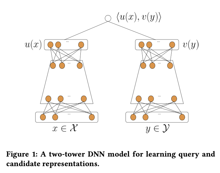
Figure 7-2. The two towers are responsible for the two embeddings
In this architecture, we take the left tower to be responsible for items, and the right tower to be responsible for user – and when appropriate – context. These two tower architectures are inspired from the NLP literature and in particular the Learning Text Similarity work.
Let’s work through in detail how this model architecture is applied to recommending videos on YouTube. For a full overview of where this architecture was first introduced, see the two-towers paper. Training labels will be given by clicks, but with an additional regression feature
As mentioned above, this model architecture will explicitly include features from both user and items. The video features will consist of categorical and continuous features, like VideoId, ChannelId, VideoTopic, and so on. An embedding layer is used for many of the categorical features to move to dense representations. The user features are things like watch histories via bag of words, and standard user features.
This model structure combines many of the ideas we’ve seen before, but has relevant takeaways for our system architecture. First, is the idea of sequential training. Each temporal batch of samples, should be trained in sequence to ensure that model drift is shown to the model; later we will discuss prequential datasets “Pre-quential validation”. Next, we see an important idea for the productionizing of these kinds of models: encoders.
In these models, we have feature encoders as the early layers in both towers, and when we move to inference, we will still need these encoders. When performing the online recommendations, we will be given UserId and VideoId, and first need to collect their features. As discussed before “Feature stores”, the Feature Store will be useful in getting these raw features, but we need to also encode into the dense representations necessary for inference. This is something that can be stored in the feature store for known entities, but for unknown entities we will need to do the feature embedding at inference time.
Encoding layers serve as a simple model for mapping a collection of features to a dense representation. When fitting encoding layers as the first step in a neural network, the common strategy is to take the first
In our previous system architecture, we would include this encoder as part of the fast layer, after receiving features from the feature store. It’s also important to note that we would still want to utilize vector search; these feature embedding layers are used upstream of the vector search and nearest neighbor searches.
Encoder as a service
As we’ve discussed briefly, and will go more deeply into, encoders and retrieval are a key part of the multi-stage recommendation pipeline. We’ve spoken briefly about the latent spaces in question “Latent Spaces”, and we’ve eluded to an encoder. Briefly, an encoder is the model which converts users, items, queries, etc. into the latent space in which you’ll perform nearest-neighbors search. These models can be trained via a variety of processes, many of which will be discussed later, but it’s important to discuss where they live once trained.
Encoders are often simple API endpoints that take the content to be embedded, and return a vector (a list of floats). Encoders often work at the batch layer to encode all the documents/items that will be retrieved, but they must also be connected to the real-time layer to encode the queries as they come in. A common pattern is to set up a batch endpoint and a single query endpoint to fascilitate optimization for both modalities. These endpoints should be fast and highly available.
In the case that you’re working with text data, a good starting place is to use BERT or GPT based embeddings, the easiest at this time are provided as a hosted service from OpenAI.
Deployment
Like many machine learning applications, the final output of a recommendation systems is itself a small program that runs continuously and exposes an API to interact with it; although batch recommendations are often a powerful place to start, performing all the necessary recommendations ahead of time. Throughout this chapter, we’ve seen the pieces embedded in our backend system, but now we will discuss the components closer to the user.
In our relatively general architecture, the server is responsible for handing over the recommendations, after all the work that comes before and it should adhere to a preset schema. But what does this deployment look like?
Models as APIs
Let’s discuss two systems architectures that might be appropriate for serving your models in production: micro-service and monolith.
In web applications this dichotomy is well covered from many perspective and special use-cases. As ML engineers, Data Scientists, and potentially Data Platform engineers, it’s not necessary to dig deep into this area, but it’s essential to know the basics. Simply: * micro-service architectures state that each component of the pipeline should be it’s own small program with clear API and output schema. Composing these API calls allows for flexible and predictable pipelines. * In contrast, monolithic architectures suggest that one application should contain all the necessary logic and components for model predictions. Keeping the application self-contained means less interfaces that need to be kept aligned and fewer rabbit holes to hunt around in when some location in your pipeline is being starved.
Whatever you choose as your strategy, you’ll need to make a few decisions:
-
How large is the necessary application? If your application will need fast access to large datasets at inference time, you’ll need to think carefully about memory requirements.
-
What access does your application need? We’ve previously discussed making use of things like Bloom filters, and Feature stores; these resources may be tightly coupled to your application – by building them in memory in the application – or they might be an API call away. Make sure your deployment accounts for these relationships.
-
Should your model be deployed to a single node or a cluster? For some types of model, even at the inference step we wish to utilize distributed computing. This will require additional configuration to allow for fast parallelization.
-
How much replication do you need? Horizontal scaling allows you to have multiple copies of the same service running simultaneously to reduce the demand on any particular instance. This is important for ensuring availability and performance. As we horizontally scale, each service can operate independently and there are different strategies for coordinating these services and an API request. Each replica is usually it’s own containerized application and things like CoreOS and Kubernetes are used to manage these. The requests themselves must also be balanced to the different replicas via something like NGINX.
-
What are the relevant API’s exposed? Each application in the stack should have a clear set of exposed schemas, and an explicit communication about what types of other applications may call to them.
Spinning up a model service
So what can you use to actually get your model into an application? One of a variety of frameworks for application development are useful; some of the most popular in Python are Flask, FastAPI, and Django. Each have different advantages, but we’ll discuss FastAPI here.
FastAPI is a targeted framework for API applications, making it especially well fit for serving ML models. It calls itself an ASGI (Asynchronous Server Gateway Interface) framework; and it’s specificity grants a ton of simplicity.
Let’s take a simple example of turning a fit torch model into a service with the FastAPI framework. First, let’s utilize an artifact store to pull down our fit model. Here we are using Weights and Biases artifact store:
importwandb,torchrun=wandb.init(project=Prod_model,job_type="inference")model_dir=run.use_artifact('bryan-wandb/recsys-torch/model:latest',type='model').download()model=torch.load(model_dir)model.eval(user_id)
This looks just like your notebook workflow, so let’s see how easy it is to integrate this with FastAPI:
fromfastapiimportFastAPI# FastAPI codeimportwandb,torchapp=FastAPI()# FastAPI coderun=wandb.init(project=Prod_model,job_type="inference")model_dir=run.use_artifact('bryan-wandb/recsys-torch/model:latest',type='model').download()model=torch.load(model_dir)@app.get("/recommendations/{user_id}")# FastAPI codedefmake_recs_for_user(user_id:int):# FastAPI codeendpoint_name='make_recs_for_user_v0'logger.info("{'type': 'recommendation_request',"f"'arguments':{'user_id':{user_id}},"f"'response':{None}},",f"'endpoint_name':{endpoint_name}")recommendation=model.eval(user_id)logger.log("{'type': 'model_inference',"f"'arguments':{'user_id':{user_id}},"f"'response':{recommendation}},"f"'endpoint_name':{endpoint_name}")return{# FastAPI code"user_id":user_id,"endpoint_name":endpoint_name,"recommendation":recommendation}
I hope you share my enthusiasm that we now have a model-as-a-service in five additional lines of code. While this scenario included some very simple examples of logging, we’ll discuss logging in greater detail later to help you improve observability in your applications.
Workflow orchestration
The other component necessary for your deployed system, is workflow orchestration. The model service is responsible for receiving requests, and serving results, but there are many components to the system that need to be in place for this service to do anything of use. There are several components to these workflows, so we will discuss them in sequence: containerization, scheduling, and CI/CD.
Containerization
Above we discussed how to put together a simple service which can return the results, and we suggested using FastAPI; however, the question of environments is now relevant. When executing Python code, the environment is important to keep consistent if not identical. FastAPI is a library for designing the interfaces, Docker is the software that manages the environment that code runs in. It’s common to hear Docker described as a container or containerization tool: this is because you load a bunch of App’s – or executable components of code – into one shared environment.
There are a few subtle things to note at this point; the meaning of environment encapsulates both the python environment of package dependencies and the larger environment like operating system or GPU drivers, the environment is usually initialized from some pre-determined image which installs the most basic aspects of what you’ll need access to and in many cases is less variable across different services to promote consistency and standardization, and finally, the container usually is equipped with a list of infrastructure code necessary to work whereever it is to be deployed.
In practice, you specify details of the python environment via your requirements file, and consists of a list of python packages – note that some library dependencies are outside python, and will require additional configuration mechanisms. The operating system and drivers are usually built as part of a base image – you can find these on DockerHub or similar. Finally, the infrastructure code is usually the necessary steps in getting your container configured to run in the infrastructure it will be deployed into. Dockerfile and DockerCompose are specific to the Docker container interfacing with infrastructure, but you can further generalize these concepts to include other details of the infrastructure. This is called infrastructure as code and begins to encapsulate provisioning of resources in your cloud, setting up open ports for network communication, access control via security roles, and more. A very common way to write this code is in Terraform. In this book, we won’t dive into infrastructure specification, but it’s becoming more and more important of a tool to the ML practitioner – many companies are beginning to attempt to simplify these aspects of training and deploying systems including Weights and Biases or Modal.
Scheduling
There are really two paradigms for scheduling of jobs – cron and triggers. Later we’ll talk more about the continuous training loop and active learning processes, but upstream of those is your ML Workflow. ML Workflows are a set of ordered steps necessary to prepare your model for inference. We’ve introduced our notion of Collector, Ranker, and Server, which are organized into a sequence of stages for Recommendation Systems – but these are the three coarsest elements of the system topology.
In ML systems, we very frequently assume that there’s an upstream stage of the workflow which corresponds to data transformations as discussed in the last chapter. Whereever that stage takes place, the output of those transformations result in our vector store – and potentially the additional feature stores. The handoff between those steps, and the next steps in your workflow are the result of a job-scheduler. As mentioned previously, tools like Dagster and Airflow, can run sequences of jobs with dependent assets. The need for these kinds of tools are to orchestrate the transitions; and to ensure that they’re timely. Cron refers to a time-schedule where a workflow should begin, for example hourly at the top of the hour, or four times a day. Triggered refers to the instigating a job run when another event has taken place. For example: if an endpoint receives a request, or a set of data gets a new version, or a limit of responses is exceeded. These are meant to capture more adhoc relationships between the next job stage and the trigger. Both paradigms are very important.
CI/CD
Your workflow execution system is the backbone of your ML systems; often the bridge between the data collection process, the training process, and the deployment process. Modern workflow execution systems also include automatic validation, and tracking so that you can audit the steps on the way to production.
Continuous Integration is a term stolen from Software Engineering to enforce a set of checks on new code to accellerate the development process. In traditional software engineering, this is comprised of automating unit and integration testing, usually run after checking the code into version control. For Machine Learning systems, CI may mean running test scripts against the model, checking the typed output of data transformations, or running validation sets through the model and benchmarking the performance against previous models.
Continuous Deployment is also a term popularlized in Software Engineering to refer to automating the process of pushing new packaged code into an existing system. In Software Engineering, deploying code when it’s passed the relevant checks speeds up development and reduces the risk of stale systems. In Machine Learning, continuous deployment can involve things like automatically deploying your new model behind a service endpoint in shadow (will discuss later this chapter) to test that it works as expected under live traffic. It could also mean to deploy it behind a very small allocation of an A/B test or Multi-arm Bandit treatment to begin to measure effects on target outcomes. Continuous Deployment usually will require effective triggering by the requirements it has to satisfy before being pushed. It’s common to hear continuous deployment utilizing a Model Registry, where you house and index variations on your model.
Alerting and Monitoring
Alerting and monitoring take a lot of their inspiration from the DevOps world for software engineering. Some high level principles which will guide our thinking are:
-
clearly defined schemas and priors
-
observability
Schemas and Priors
When designing software systems, you almost always have expectations of how the components fit together. Much like in writing code where you anticipate the input and output to functions, in software systems you anticipate these at each interface. This is relevant not only for micro-service architectures; even in a monolith architecture components of the system need to work together and often will have boundaries between their defining responsibilities.
Let’s make this more concrete via an example: you’ve built a user-item latent space, a feature store for user features, a bloom filter for client avoids, and an experiment index which defines which of two models should be used for scoring. First let’s examine the latent space: when provided a user_id we need to look up its representation, and we have some assumptions already:
-
user_idprovided will be of the correct type -
user_idwill have a representation in our space -
The representation returned will be of the correct type and
shape -
The component values of the representation vector will be in the appropriate domain. (Note: the support of representations in your latent space may vary day-to-day)
From here, we need look up the
-
There are
-
Those vectors adhere to the expected distributional behavior of the latent space
While these seem relatively straightforward application of unit-tests, canonizing these assumptions is important. Take the last assumption in both of the two services: how can you know the appropriate domain for the representation vectors? As part of your training procedure, you’ll need to calculate this, then store it for access during the inference pipeline.
In the second case, when finding nearest neighbors in high dimensional spaces, there are well discussed difficulties in distributional uniformity, but this can mean particularly poor performance for recommendations. In practice, we have observed a spiky nature to the behavior of
In both cases, collecting the output of this information and logging it can provide a rich history of what is going on with your system. This can shorten debugging loops later on if model performance is low in production.
Returning to the possibility of user_id lacking a representation in our space: this is precisely the cold-start problem! In that case we need to transition over to a different prediction pipeline: perhaps user-feature-based, explore-exploit, or even hard-coded recommendations. In this setting, we need understand next steps when a schema condition is not met and gracefully move forward.
Integration tests
Let’s consider one higher-level challenge that might emerge in a system like this at the level of integration. Some refer to these issues as entanglement.
You’ve learned through experimentation that you should find
Naively, if you take the 20 neighbors, and pass them into the bloom, you’re likely to be left with nothing! There are two ways to approach this challenge:
-
allow for a call-back from the filter step to the retrieval (c.f. “Predicate pushdown”)
-
build a user-distribution and store that for access during retrieval
In the first of these, you give access to your filter step to call the retrieval step with a larger
In the second of these, during training, you can sample from the user space to build estimates of the appropriate
Observability
There are quite a number of tools in the software engineering to assist with observability, understanding the why’s of what’s going on in the software stack. Because the systems we are building become quite distributed, the interfaces become critical monitoring points, but the paths also become complex.
Common terms in this area are spans and traces, which refer to two dimensions of a call stack. Given some collection of connected services, like in our above examples, an individual inference request will pass through some or all of those services in a sequence. The sequence of service requests is the trace. The, potentially parallel, time-delays of each of these services, is the span.

Figure 7-3. TODO: Need to remake from scratch
The graphical representation of spans usually demonstrates how the time for one service to respond is comprised of several other delays from other calls.
Observability enables you to see traces, spans, and logs in conjunction to appropriately diagnose the behavior of your system. In our example above where we utilize a call-back from the filter step to get more neighbors from the collector, we might see a slow response and wonder “what has happened?”. By viewing the spans and traces, we’d be able to see that the first call to the collector was as expected, then the filter step made a call to the collector, then another call to the collector, and so on, which built up a huge span for the filter step. Combining that view with logging would help us rapidly diagnose what might be happening.
Time-outs
In the above example, we had a long process that could lead to a very bad user experience. In most cases, we impose hard restrictions on how bad we let things get; these are called time-outs.
Usually we have an upper bound on how long we’re willing to wait for our inference response, and so implementing time-outs aligns our system with these restrictions. It’s important in these cases to have a fall-back. In the setting of recommendation systems, a fall-back is usually comprised of things like the Most Popular Item Recommender prepared such that it incurs minimal additional delay.
Evaluation in Prod
If the previous section was understanding what’s coming into your model in production, this might be summarized as what’s coming out of your model in production. At a high level, evaluation in prod can be thought of as extending all your model validation techniques to the inference time. In particular, what the model actually is doing!
On one hand we already have tools to do this evaluation – you can use the same methods used for evaluating performance as in training, but now on real observations streaming in. However, this is not as obvious as we might first guess. Let’s discuss some of the challenges.
Slow feedback
Recommendation systems fundamentally are trying to lead to item selection, and in many cases, purchases. But if we step back and think more holistically about how recommendation systems integrate into businesses, it’s to drive revenue. If you’re an e-commerce shop, item selection and revenue may seem easily associated: a purchase leads to revenue, so good item recommendation leads to revenue. However, what about returns? Or even a harder question: are these revenue incremental? One challenge with recommendation systems, is there may sometimes be a very difficult to draw causal arrow between any metric used to measure the performance of your models to the business-oriented key performance indicators.
We call this slow feedback because sometime the loop to get from a recommendation, to a meaningful metric, and back to the recommender can take weeks or even longer. This is especially challenging when you want to run experiments to understand if a new model should be rolled out. The length of the test may need to stretch quite a bit more to get meaningful results.
Usually a proxy metric is aligned on that the data scientists believe is a good estimator for the KPI, and that proxy metric is measured live. There are a huge variety of challenges with this approach, but it often suffices and provides motivation for more testing. Well correlated proxies are often a great start to get directional information on where to take further iterations.
Model metrics
So what are the key metrics to track for your model in prod? Given that we’re looking at recommendation systems at inference time, we should seek to understand:
-
distribution of recommendation across categorical features
-
distribution of affinity scores
-
number of candidates
-
distribution of other ranking scores
As we discussed before, during the training process, we should be calculating broadly what the ranges of our similarity scores are in our latent space. Whether we are looking at high level estimations, or finer ones, we can use these distributions to get warning signals something might be strange. Simply comparing the output of our model during inference, or over a set of inference requests, to these pre-compute distributions can be extremely helpful.
Comparing distributions can be a long topic, but one standard approach is KL-Divergence between the observed distribution, and the expected distribution from training. By computing KL-Divergence between these, we can understand how surprising the model’s predictions are on a given day.
What we’d really like is to understand the ROC(Receiver Operating Curve of your model predictions with respect to one of your conversion types. However, this involves yet another integration to tie back to logging. Since your model API only produces the recommendation, you’ll still need to tie into logging from the web application to understand outcomes! To tie back in outcomes one must join the model predictions with the logging output to get the evaluation labels, which can be done via log parsing technologies (like graphana, ELK, or Prometheus). We’ll see more of this in the next chapter.
Continuous training and deployment
It may feel like we’re done with this story since we have models tracked and production monitoring in place, but rarely are we satisfied with set-it-and-forget-it of model development. One important characteristic of ML products, is how models frequently need to be updated to even be useful. Above we discussed model metrics, and how sometimes performance in production might look different than what we had come to expect from the trained models’ performance. This can even be further exacerbated by model drift.
Model drift is the notion that the same model may exhibit different prediction behavior over time, merely due to changes in the data generating process. A very simple example is a time-series forecasting model. When you build a time-series forecast model, the especially unique property that is essential for good performance is auto-regression, that is to say that the value of the function covaries with previous values of the function. We won’t go into detail on time-series forecasting, but suffice to say: the best hope you have of making a good forecast is to use up-to-date data! If you wanted to forecast stock prices, you’d always want to use the most recent prices as part of your predictions. This simple example demonstrates how models may drift, and forecasting models are not so different than recommendation models – especially when considering the seasonal realities of many recommendation problems. A model that did well two weeks ago, needs to be retrained with recent data to be expected to continue to perform well.
One criticism of a model that drifts is “that’s the smoking gun of an overfit model”, but in reality these models require a certain amount of over-parameterization to be useful models. In the context of recommendation systems, we’ve already seen things like the Matthew Effect have disastrous effects on the expected performance of a recommender model. If we don’t consider thinks like new items in our recommender, we are doomed to fail. Models can drift for a variety of reasons, often coming down to exogenous factors in the generating process that may not be captured by the model.
One approach to dealing with and predicting stale models, is to simulate these scenarios during training. If your expectation is that the model goes stale mostly due to the distribution changing over time, you can employ sequential cross-validation – i.e. train on a contiguous period and test on a subsequent period – but with a specified block of time delay. For example, if you think your model performance is going to decrease after two week due to being trained on out-of-date observations, then during training you can purposely build your evaluation to incorporate a two-week delay before measuring performance. This is called two-phase prediction comparison and by comparing the performances you can estimate drift magnitudes to keep an eye out in prod.
There are a wealth of statistical approaches to reigning in these differences. In lieu of a deep dive into variational modeling for variability and reliability for your predictions, we’ll instead discuss continuous training and deployment and open this peanut with a sledge hammer.
Deployment topologies
Let’s consider a few different structures for how you want to deploy models to not only keep your models well in tune, but to accommodate iteration, experimentation, and optimization.
Ensembles
Ensembles are a type of model structure in which multiple models are built, and the predictions from those models are pooled together in one of a variety of ways. While this notion of an ensemble is usually packaged into the model called for inference, you can actually generalize the idea to your deployment topology. Let’s take an example that builds on our previous discussion of prediction priors. If we have a collection of models with comparable performance on a task, we can deploy them in ensemble weighted by their deviation from the prior distributions of prediction that we’ve set before. This way, instead of having a simple yes/no filter on the output of your model’s range, you can more smoothly transition potentially problematic predictions into more expected ones.
Another benefit of treating the ensemble as a deployment topology instead of only a model architecture, is that you can hot-swap components of an ensemble as you make improvements in specific sub-domains of your observation feature space. Take for example an LTV model comprised of three components, one that predicts well for new clients, another for activated clients, and a third for super-users. You may find that pooling via a voting mechanism on average performs the best, so you decide to implement a bagging approach. This works well, but later you find a better model for the new clients. By using deployment topology for your ensemble you can swap in the new model for the new clients, and start comparing performance in your ensemble in prod. This brings us to the next strategy, model comparison.
Shadowing
Deploying two models, even for the same task, can be enormously informative. We call this shadowing in the case where one model is “live” and the other is secretly also receiving all the requests and doing inference, and logging the results of course. By shadowing traffic to the other model, you get the best expectations possible about how the model behaves before making your model live. This is especially useful when wanting to ensure that the prediction ranges align with expectation.
In software engineering and devOps, there’s a notion of staging for software. It’s a hotly contested question of “how much of the real infra should staging see”, but shadowing is the staging of ML models. You can basically build a parallel pipeline for your entire infrastructure to connect for shadow models, or you can just put them both in the line of fire and have the request sent to both, but only use one response. Shadowing is also crucial for implementing experimentation.
Experimentation
As good data scientists, we know that without a proper experimental framework, it’s risky to advertise much about the performance of a feature or in this case model. Experimentation can be handled with shadowing by having a controller layer that is taking the incoming requests and orchestrating which of the deployed models to curry the response along from. A simple A/B experimentation framework might ask for a randomization at every request, where-as something like a multi-armed bandit will require the controller layer to have notions of the reward function.
Experimentation is a deep topic which we don’t have the knowledge or space to do adequate justice, but it’s useful to know that this is where experimentation can fit into the larger deployment pipeline.
The evaluation flywheel
By now it’s likely obvious that a production ML model is far from a static object. Production ML systems of any kind are subject to as many deployment concerns as a traditional software stack, in addition to the added challenge of dataset shift and new users/items. In this section we want to look closely at the feedback loops introduced and understand how the components fit together to continuously improve our system–even with little input from a data scientist or ML Engineer.
Daily warm-starts
As we’ve now discussed several times, there needs be a connection between the continuous output of our model and retraining. The first simplest example of this is daily warm-starts, which essentially asks us to utilize the new data seen each day in our system.
As might already be obvious, some of the recommendation models that show great success are quite large. Retraining some of them can be a massive undertaking, and simply rerunning everything each day is often infeasible. So what can be done?
Let’s ground this conversation in the user-user collaborative filtering example that we’ve been sketching out; we have seen that the first step was to build an embedding via our similarity definition. Let’s recall:
here we remember that the similarity between two users is dependent on the shared ratings, and by each user’s average rating.
On a given day, let’s consider
This is a bit ad-hoc, but for many methods you can utilize these tricks to reduce a full retraining. This would avoid a full batch retraining, via a fast-layer. There are other approaches to this like building a separate model that can approximate recs for low-signal items. This can be done via feature models, and can significantly reduce the complexity of these quick re-trainings.
Lambda architecture and orchestration
On the more extreme end of the spectrum of these strategies is the lambda architecture; as discussed during our data hydration discussions, the lambda architecture seeks to have a much more frequent pipeline for adding new data into the system. The speed layer is responsible for working on small batches to perform the data transformations, and model fitting to combine with the core model. As a reminder, there are many other aspects of the pipeline that should also be updated during these fast layers, like the nearest neighbors graph, the feature store, and the filters.
Different components of the pipeline can require different investments to keep updated, so the schedules they are on are an important consideration. You might be starting to notice that keeping all of these things in sync can be a bit challenging–if you have model training, model updating, feature store updates, redeployment, and new items/users all coming in on potentially different schedules, there can be a lot of coordination necessary. This is where an orchestration tool can become relevant. There are a variety of approaches but a few useful technologies here are GoCD, MetaFlow, and KubeFlow; the latter being more oriented at Kubernetes infrastructures. Another pipeline orchestration tool that can handle both batch and streaming pipelines is Apache Beam.
Generally, for ML deployment pipelines we need to have a reliable core pipeline, and the ability to keep things up-to-date as more data pours in. Orchestration systems usually define the topology of the systems, the relevant infrastructure configurations, the mapping of the code artifacts needing to be run, and the CRON schedules when all as code itself. Code-as-infrastructure is a popular paradigm which captures these goals as a mantra, so that even all of this configuration itself is reproducible and automatable.
In all of the above, there’s a heavy overlap with containerization and how these things may be deployed. Unfortunately most of this discussion is beyond the scope of this book, but a simple overview is that containerized deployment with something like Docker is extremely helpful for ML Services and managing those deployments with various container management systems, like Kubernetes, is also popular.
Logging
Logging has come up several times already. In model monitoring and our schema assumptions sections we saw that logging was very important for insuring that our system was behaving as expected. Let’s discuss some best practices for logging, and how they fit into our plans.
When we discussed traces and spans earlier, we were able to get a snapshot of the entire call-stack of the services involved in responding to a request. This concept of linking together the services to see the larger picture is incredibly useful, and when it comes to logging gives us a hint as to how we should be orienting our thinking. Returning to our favorite RecSys architecture we have:
-
Collector receiving the request and looking up the embedding relevant to the user
-
Computing ANN on items for that vector
-
Applying filters via blooms to eliminate potential bad recs
-
Feature augmentation to the candidate items and user via the feature stores
-
Scoring of candidates via the ranking model, and potential confidence estimation
-
Ordering and application of business logic or experimentation
Each of the above have potential applications of logging, but let’s now think about how to link them together. The relevant concept from microservices is that of correlation IDs which is simply an identifier that’s passed along the call stack to ensure the ability to link everything later. As is likely obvious at this point, each of these services will be responsible for their own logging, but they’re almost always more useful in aggregate.
These days, Kafka is often used as the log-stream processor to listen for logs from all of the services in your pipeline, and manage their processing and storing. Kafka relies on a message-based architecture where each service is a producer and Kafka helps manage those messages to consumer channels. In terms of log management, the Kafka cluster receives all of the logs in the relevant formats, hopefully augmented with correlation IDs, and sends them off to what’s called an ELK stack. The ELK stack–Elastic Search, LogStash, Kibana–consists of a Logstash component to handle incoming log streams and apply structured processing, Elastic Search which builds search indices to the log store, and Kibana which adds a UI and high level dashboarding to the logging.
This stack of technologies is focused at ensuring you have access and observability from your logs, and there are others that focus on other aspects, but what should you be logging?
Collector logs
Again, we wish to log during the:
-
collector receiving the request and looking up the embedding relevant to the user
-
computing ANN on items for that vector.
The collector receives a request, consisting in our simplest example of user_id, requesting_timestamp, and any augmenting kwargs that might be required. A correlation_id should be passed along from the requester, or generated at this step. A log with these basic keys should be fired, along with the timestamp of request received. A call is made to the embedding store and the collector should log this request. Then the embedding store should log this request when received, along with the embedding store’s response. Finally the collector should log the response as it returns. This may feel like a lot of redundant information but the explicit parameters included in the API calls become extremely useful when troubleshooting.
The collector now has the vector it will need to perform a vector search, so it will make a call to the ANN service. Logging this call, and any relevant logic in choosing the
At this point, we have at least 6 logs emitted–only reinforcing the need for a way to link these all together. In practice, you often have other relevant steps in your service that should be logged; e.g. checking that the distribution of distances in returned neighbors is appropriate for downstream ranking.
Note that if the embedding lookup was a miss, it’s obviously important to log that, and log the subsequent request to the cold-start recommendation pipeline. This will also incur additional logs as it moves through that.
Filtering and Scoring
Now we need to monitor the following steps:
-
Applying filters via blooms to eliminate potential bad recs
-
Feature augmentation to the candidate items and user via the feature stores
-
Scoring of candidates via the ranking model, and potential confidence estimation.
We should log the incoming request to the filtering service, and we should log the collection of filters we wish to apply. Additionally, as we search the blooms for each item and rule them in our out of the bloom, we should build up some structured logging of which items are caught in which filters, and log all of this as a blob for later inspection. Response and request should be logged as part of feature augmentation – where we should log requests and responses to the feature store. Also log the augmented features that end up attached to the item entities. This may seem redundant with the feature store itself, but understanding what features were added during a recommendation pipeline is crucial in looking back later for why the pipeline might behave differently than anticipated. At the time of scoring, the entire set of candidates should be logged with the features necessary for scoring and the output scores. It’s extremely powerful to log this entire dataset, because training later can use these to get a better sense for real ranking sets. Finally, the response passing off to the next step with the ranked candidates and all their features.
Ordering
We’ve got one more step to go, but it’s an essential one: ordering and application of business logic or experimentation.
This step is probably the most important logging step, because of how complicated and ad-hoc the logic in this step can get. If you have multiple intersecting business requirements implemented via filters at this step, while also integrating with experimentation, you can find yourself seriously struggling to unpack how reasonable expectations coming out of the Ranker have turned into a mess by response time. Things like logging the incoming candidates, keyed to why they’re eliminated, and the order of business rules applied will make this much more tractable.
Additionally, experimentation routing will likely be handled by another service, but what experiment id was seen in this step, and how that experiment assignment was utilized are providence of the Server. As we ship off the final recs, or decide to go another round, one last log of the state of the recommendation will ensure that app logs can be validated with response.
Active Learning
So far we have discussed using updating data to train on a much more frequent schedule, and we’ve discussed how to provide good recommendations, even when the model hasn’t seen enough data for those entities. However, there’s a further opportunity for the feedback loop of recommendation and rating, and that’s active learning.
We wont be able to go deep into the topic, which is a large and active field of research, but we will discuss the core ideas in relation to recommendation systems. Active learning changes the learning paradigm a bit by suggesting that the learner should not only be passively collecting labeled–maybe implicit–observations, but also be attempting to mine relations and preferences from them. Active learning determines what data and observations would be most useful in improving model performance, and then seeks out those labels. In the context of RecSys, we know that the Matthew Effect is one of our biggest challenges, in that many of potentially good matches for a user may be lacking enough or appropriate ratings to bubble to the top during the recommendations.
What if we employed a simple policy: every new item to the store gets recommended as a second option to the first 100 customers. The outcome would be two things:
-
we would quickly establish some data for our new item to help cold-start it
-
we would likely decrease the performance of our recommender.
In many cases, the second outcome is worth enduring to achieve the first, but when? And is this the right way to approach this problem? Active learning provides a methodical approach to these problems.
Another more specific advantage of active learning schemes is that you can broaden the distribution of observed data. In addition to just cold-start items, one can use active learning to target broadening users interests. This is usually framed as an uncertainty reduction technique, as it can be used to improve the confidence in recommendations in a broader range of item categories. A simple example here would be if a user only ever shops Sci-Fi books, so one day you show them a few extremely well liked Westerns to ascertain if that user might be open to getting Westerns recommended to them some times. “Propensity Weighting for Recommendation System Evaluation”
An active learning system is instrumented as a loss function inherited from the model it’s trying to enhance–usually tied to uncertainty in some capacity–and it’s attempting to minimize that loss. Given a model
The structure of an active learning system roughly follows the following steps:
-
Estimate marginal decrease in loss due to obtaining one of a set of observations
-
Select the one with the largest effect
-
Query the user; i.e. provide the recommendation to obtain a label
-
Update the model.
It’s probably clear that this paradigm requires a much faster training loop than our previous fast retraining schemes. Active learning can be instrumented in the same infrastructure as our other setups, or have its own mechanisms for integration into the pipeline.
Types of optimization
There are two approaches to the optimization procedure carried out by an active learner in a recommendation system: personalized and non-personalized. Because RecSys is all about personalization, it’s no surprise that we would, in time, want to push the utility of our active learning further by integrating the great things we already know about users.
We can think of these two approaches as split between global loss minimization or local loss minimization. Active learning that isn’t personalized tends to be about minimizing the loss over the entire system, not only for one user. Warning, this split doesn’t perfectly capture the ontology, but it’s a useful mnemonic. In practice, optimization methods are nuanced and sometimes utilize very complicated algorithms and training procedures.
Let’s talk through some things to optimize with respect to for non-personalized active learning:
-
User rating variance, consider which items have the largest variance in user ratings to try to get more data on those we find the most complicated in our observations
-
Entropy, the dispersion of ratings of a particular item across an ordinal feature. This is useful for understanding how uniform random our set of ratings for an item is
-
Greedy extend, a measurement for which items seem to yield the worst performance in our current model; this attempts to improve our performance overall by collecting more data on the hardest items to recommend well
-
Representatives or exemplars, picking out items which are extremely representative of large groups of items; we can think of this as “if we’ve got good labels for this, we’ve got good labels for everything like this”
-
Popularity, select items most likely for the user to have experience with to maximize the likelihood that they have an opinion or rating to give
-
Co-coverage, attempting to amplify the ratings for frequently occurring pairs in the dataset; this strikes directly at the collaborative filtering structure to maximize the utility of observations
On the personalized side:
-
Binary prediction, to maximize the chances that the user can provide the requested rating we can choose the items that the user is more likely to have experienced. This can be achieved via a MF on the binary ratings matrix.
-
Influence based, targeted at estimating the influence of item ratings on the rating prediction of other items and selects the items with the largest influence. This attempts to directly measure the impact of a new item rating on the system.
-
Rating optimized, obviously there’s an opportunity to simply use the best rating or best rating within some class to perform active learning queries, but this is precisely the standard strategy in recommendation systems to serve good recommendations.
-
User segmented, when available, user-segmentation and feature clusters within users can be used to anticipate when user’s have opinions and preferences on an item by virtue of the user-similarity structure.
In general, there’s a soft trade-off between active learning useful for maximally improving your model globally, and maximizing the likelihood that a user can and will rate a particular item.
Let’s look at one particular example that uses both.
Application: User Sign-up
One common hurdle to overcome in building recommendation systems is on-boarding new users. By definition, new users will be cold starting with no ratings of any kind, and will likely not expect great recommendations from the start.
We may begin with the MPIM for all new users–simply show them something to get them started and then learn as you go. But is there something better?
One approach you’ve probably experienced is the user on-boarding flow; a simple set of questions employed by many websites to quickly ascertain some basic information about the user, to help quickly guide early recommendation. If discussing our book recommender, this might be asking what genres the user likes, or in the case of a coffee recommender: how they brew their coffee in the morning. It’s probably clear that these are building up knowledge-based recommender systems and don’t directly feed into our previous pipelines, but can still provide some help in early recommendations.
If instead, we looked at all of our previous data and asked: “which books in particular are most useful for determining a user’s taste"–this would be an active learning approach. We could even have a splitting tree of possibilities as they answered each question wherein the answer determines which next question is most useful to ask.
Summary
Now we have the confidence that we can serve up our recommendations, and even better we have instrumented our system to gather feedback. We’ve seen how you can gain confidence before you deploy, and we’ve seen how you can experiment with new models or solutions. Ensembles and cascades allow you to combine testing with iteration, and the data flywheel provides a powerful mechanism for improving your product.
You may be finding yourself wondering how to put all these new learnings into practice, to which the next chapter will speak. Let’s understand how data processing and simple counting can lead to an effective – and useful! – recommendation system.