Sharding

Sharding is probably the simplest strategy to divide and conquer. Suppose you have K machines, N items and M users. Using a sharding strategy you can reduce the runtime to O(N * M / K). You can do this by assigning each item with a unique identifier, so you have tuples of (unique_id, item_vector). Then, by simply taking machine_id = unique_id % K, one can assign a subset of the corpus to a different machine. When the a user needs a recommendation, one can then compute either ahead of time or on demand the top scoring recommendations by distributing the workload onto K different machines and thus make the computation K times faster, except for some overhead in gathering the top results on the server and ordering them jointly. Note that if you want say 100 top scoring items, you would still have to obtain the top 100 results from each shard, collate them together and then sort all the results jointly if you want to have the same results as in a brute force method of scoring the entire corpus.

Sharding is useful in the sense that it can be combined with any of the other acceleration methods and is not dependent on the representation having any specific form such as being a single vector.

Locality Sensitive Hashing

Locality Sensitive Hashing (LSH) is an interesting technique in that it converts a vector into a token based representation. This is powerful because if CPUs are readily available then one can use them to compute the similarity between vectors using cheaper integer arithmetic operations such as XOR and bit counting with specialized assembly instructions rather than floating point operations. Integer operations tend to be much faster on CPUs than floating point operations, so one is able to compute similarity between items much faster than using vector operations. The other benefit is that once items are represented as a series of tokens, then a regular search engine database would be able to store and retrieve these items using token matching. Regular hashing on the other hand tends to result in vastly different hash codes if there is a slight change in the input. This is not a criticism of the hash functions, they just have different uses for different kinds of data.

Let’s walk though a couple ways of how to convert a vector into a hash. Locality sensitive hashing is different from regular hashing in that small perturbations to a vector should result in the same hash bits as the hash of the original vector. This is an important property as it allows us to look up the neighborhood of a vector using very fast methods such as hash maps. One very simple hashing method is called The Power of Comparitive Reasoning or Winner Take All hashing. In this hashing scheme, the vector is first permuted using a known, reproducible permutation. One can generate this known permutation by simply shuffling the indices of all the vector dimensions with a random number generator that accepts a seed and reliably reproduces the same exact shuffle sequence. It is important that the permutation is stable over different versions of python as one wants to reproduce the hashing operation when generating the hashes as well as in retrieval time. Since we are using JAX’s random library and JAX is careful about the reproduciblity of permutations, we just directly use the permutation function in JAX. The hash code computation after that is simply a comparison between adjacent dimensions of the permuted vector as follows.

def compute_wta_hash(x):
  """Example code to compute some Winner take all hash vectors
  Args:
    x: a vector
  Result:
    hash: a hash code
  """
  key = jax.random.PRNGKey(1337)
  permuted = jax.random.permutation(key, x)

  hash1 = permuted[0] > permuted[1]
  hash2 = permuted[1] > permuted[2]

  return (hash1, hash2)

x1 = jnp.array([1, 2, 3])
x2 = jnp.array([1, 2.5, 3])
x3 = jnp.array([3, 2, 1])
x1_hash = compute_wta_hash(x1)
x2_hash = compute_wta_hash(x2)
x3_hash = compute_wta_hash(x3)
print(x1_hash)
print(x2_hash)
print(x3_hash)

(Array(False, dtype=bool), Array(True, dtype=bool))
(Array(False, dtype=bool), Array(True, dtype=bool))
(Array(True, dtype=bool), Array(False, dtype=bool))

As you can see the vector x2 is slightly different from x1 and results in the same hash code of 01, whereas, x3 is different and results in a hash code of 10. The Hamming distance of the hash code is then used to compute the distance between two vectors. It is simply the XOR of the two hash codes, which results in 1 whenever the bits disagree, followed by bit counting.

x = 16
y = 15
hamming_xy = int.bit_count(x ^ y)
print(hamming_xy)
5

Using Hamming distance as shown in Example 16-2 results in some speedup in the distance computation, but the major speedup will come from the use of using the hash codes in a hash map. For example, one could break up the hash code into 8-bit chunks, and store the corpus into shards keyed by each 8-bit chunk, which results in a 256x speedup because one only has to look in the hash map which has the same key as the query vector for nearest neighbors. This has a drawback in terms of recall though, because all 8 bits have to match in order for an item to be retrieved that matches the query vector. There is a tradeoff between the number of bits of the hash code used in hashing vs hamming distance computation. The larger the number of bits, the faster the search, because the corpus is divided into smaller and smaller chunks. However, the drawback is that more and more bits have to match and thus some nearby vector in the original space might not have all the bits in their hash code match and so might not be retrieved. The remedy to this is to have multiple hash codes with different random number generators and repeat this process a few times with different random seeds. This extra step is left as an exercise to the reader.

Another common way to compute hash bits uses something called the Johnson-Lindenstrauss Lemma, which is a fancy way of saying that two vectors, when multiplied by the same random Gaussian matrix, tend to end up in a similar location when multiplied by that matrix. However, if one were to read the text of the lemma, the L2 distances are preserved, which means this hash function works better if one was using Euclidean distance to train the embeddings rather than dot products. In this scheme, only the hash code computation differs, the Hamming distance treatment is exactly the same. The speedup from LSH is directly proportional to the number of bits of the hash code that has to be an exact match. Suppose only 8-bits of the hash code are used in the hash map, then the speedup is 2^8 or 256 times the original. The tradeoff for the speed is having to store the hash map in memory.

K-d Trees

A very common strategy for speeding up computation in computer science is called divide and conquer. In this scheme, the data is recursively partitioned into two halves and only the half which is relevant to the search query is searched. In contrast to a linear O(n) in the number of items in the corpus scheme, a divide and conquery algorithm would be able to query a corpus in O(log2(n)) time, which is a substantial speedup if n is large.

One such binary tree for vector spaces is called a K-d tree. Typically, to build a K-d tree, one computes the bounding box of all the points in the collection, finds the longest edge of the bounding box and splits it down the middle of that edge in the splitting dimension then partitions the collection into two halves. If the median is used, the collection is more or less divided into two equal numbered items, the more or less is due to the fact that there might be ties along that split dimension. The recursive process stops when there is a small number of items left in the leaf node. There are many implementations of K-d trees, for example Scipy’s K-d tree. Although the speedup is substantial, this method tends to work when the number of feature dimensions of the vector is low. Also, similar to other methods, K-d trees work best when the L2 distance is the metric used for the embedding. There might be losses in retrieval if dot product was used for the similarity metric as the K-d tree makes more sense for Euclidean space partitioning.

Example 16-3 provides sample code on how one might split a batch of points along the largest dimension.

import jax
import jax.numpy as jnp

def kdtree_partition(x: jnp.ndarray):
  """Finds the split plane and value for a batch of vectors x."""
  # First, find the bounding box.
  bbox_min = jnp.min(x, axis=0)
  bbox_max = jnp.max(x, axis=0)
  # Return the largest split dimension and value.
  diff = bbox_max - bbox_min
  split_dim = jnp.argmax(diff)
  split_value = 0.5 * (bbox_min[split_dim] + bbox_max[split_dim])
  return split_dim, split_value

key = jax.random.PRNGKey(42)
x = jax.random.normal(key, [256, 3]) * jnp.array([1, 3, 2])
split_dim, split_value = kdtree_partition(x)
print("Split dimension %d at value %f" % (split_dim, split_value))

# Partition the points into two groups, the left subtree
# has all the elements left of the splitting plane.
left = jnp.where(x[:, split_dim] < split_value)
right = jnp.where(x[:, split_dim] >= split_value)

Split dimension 1 at value -0.352623

As you can see from the code, the kd-tree partitioning code can be as simple as splitting along the middle longest dimension. Other possiblities are splitting along the median of the longest dimension or Using a surface area heuristic.

Figure 16-1. KD-Tree construction initial bounding box

Figure 16-1 A KD-Tree is constructed by repeately partitioning the data along only one spatial dimension (usually along the largest axis aligned spread of data) at a time.

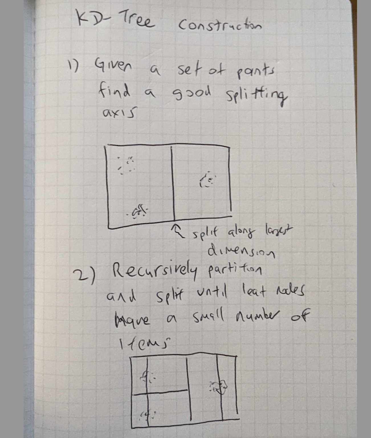
Figure 16-2. KD-Tree construction recursively partitioned

Figure 16-2 Partitions are recursively subdivided again, usually along the longest axis, until the number of points in the partition are less than a chosen small number.

The K-d tree lookup time is O(log2(n)) in n, the number of items in the corpus. It also requires some small overhead of memory to store the tree itself which is dominated by the number of the leaf nodes, so it would be best to have a minimal number of items in a leaf to prevent too fine of splits.

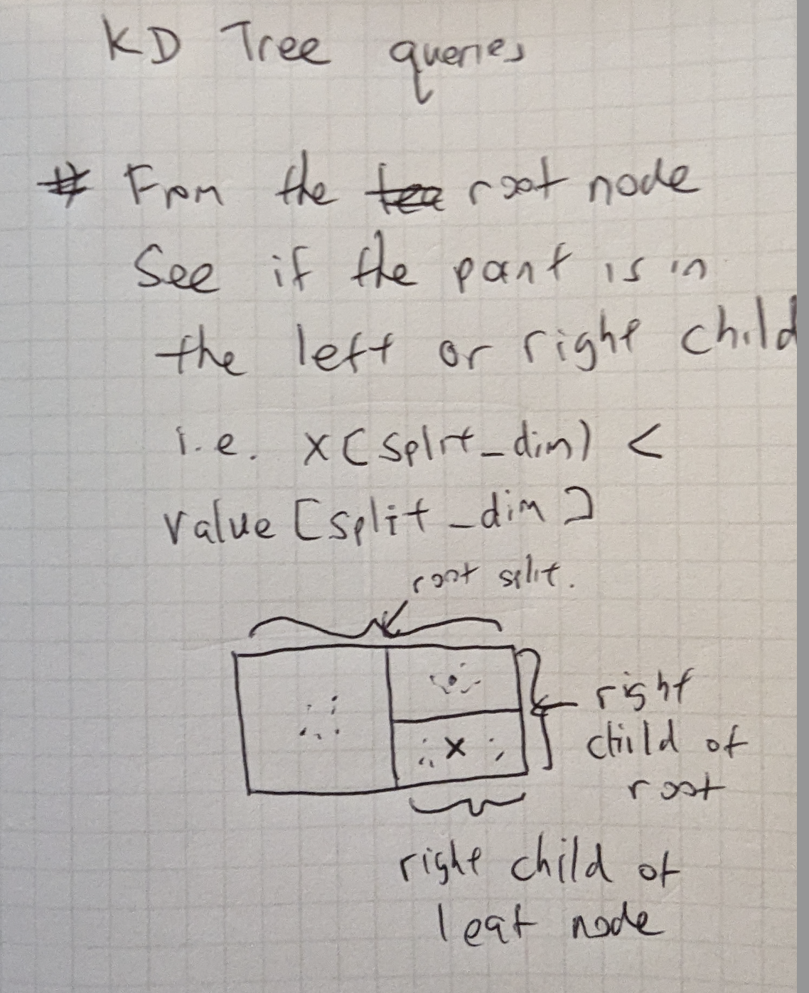
Figure 16-3. KD-Tree Query

Figure 16-1 From the root node, repeatedly check if the query point (e.g. the item we are looking for nearest neighbors for) is in the left or right child of the root node. For example, go_left = x[split_dim] < value_split[dim]. In binary tree convention, left child is usually when the query point’s split dimension value is less than the splitting plane’s value and the right child contains all points whose value at the split dimension is larger than the split value. Recursively descend down the tree until the leaf node, then exhaustively compute distances to all items in the leaf node.

A potential drawback of a K-d tree is if an item is close to a splitting plane, it would be considered on the other side of the tree. As a result, it would not considered as a nearest neighbor candidate. In some implementations of K-d trees, called spill trees, both sides of a splitting plane are visited if the query point is close enough to the decision boundary of the splitting plane. This change increases runtime a little bit for the benefit of more recall.

Hierarchical K-means

Another divide and conquer strategy that does scale to higher feature dimensions is called K-means clustering. In this scheme, the corpus is clustered into K clusters and then recursively clustered in to K more clusters until each cluster is smaller than some defined limit.

An implementation of K-means can be found at Scikit learn’s webpage.

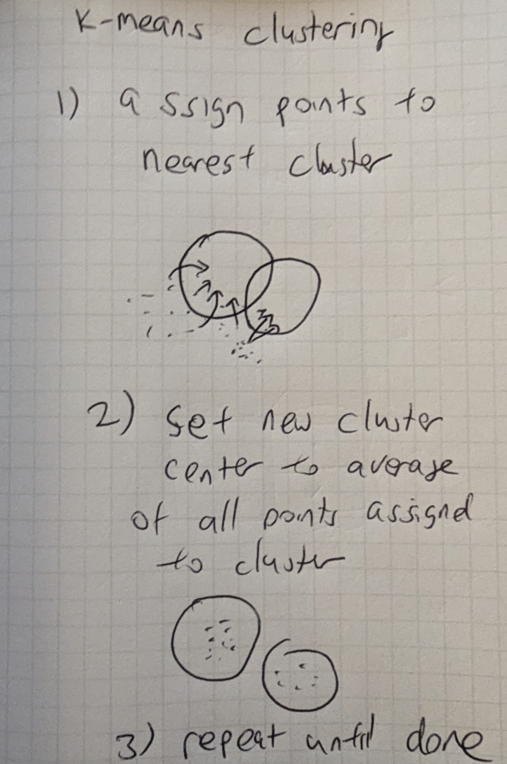
Figure 16-4. KMeans Initialization

Figure 16-4 We first create cluster centroids at random from existing points.

Figure 16-5. KMeans Clustering

Figure 16-5 Next, we assign all points to the cluster they are closest to. Then for each cluster, we take the average of all the assigned points as the new cluster center. We repeat until done, which can be a fixed number of steps. The output is then K cluster centers of points. The process can be repeated again for each cluster center splitting again into K more clusters.

Again the speedup is O(log(n)) in the number of items, but K-means is better adapted to clustering higher dimensional data points than K-d trees.

The querying for a K-Means cluster is rather straightfoward. You can find the closest cluster to the query point and then repeat the process for all subclusters until a leaf node is found and then all the items in the leaf node are scored against the query point.

An alternative to the K-means is to perform Singular Value Decomposition (SVD) and use the first K eigenvectors as the clustering criteria. The use of SVD is interesting in that there exists closed form and approximate methods like Power Iteration for computing the eigenvectors. Using the dot product to compute affinity might be better suited to vectors trained using dot product as the affinity metric.

To learn more on this topic, you can consult this paper by one of the authors where they compared LSH, SVD and Hierchical K-means Label partitioner for Sublinear Ranking. You’ll find a comparison between the speedup with the loss in retrieval with the brute-force as a baseline.

Cheaper Retrieval Methods

If your corpus has the ability to do an item wise cheap retrieval method, one way to speed things up is to do the cheap retrieval method to obtain a small subset of items and then use the more expensive vector based methods to rank the subset. One such cheap retrieval method is to make a posting list of the top co-occurrences of one item with another. Then when it comes to generating the candidates for ranking, gather all the top co-occuring items together (from a user’s preferred items for example) and then score them together with the machine learning model. In this way we do not have to score the entire corpus with the machine learning model, but just a small subset.

Conclusions

In this chapter we showed a few ways you can use to speed up the retrieval and scoring of items in a corpus given a query vector without losing too much in terms of recall while still maintaining precision. There is no perfect approximate nearest neighbor method as the acceleration structures depend on the distribution of the data and this varies from dataset to dataset. We hope that this chapter provides a launching pad for you to explore various ways in which to make retrieval faster and sublinear in the number of items in the corpus.