Zipf’s laws in RecSys and the Matthew Effect

In a great many applications of machine learning a caveat is given early: that the distribution of observations of unique items from a large corpus is modeled by Zipf’s law, i.e. the frequency of occurrence drops of exponentially. In recommendation systems, the Matthew Effect appears in the popular item’s click rates, or the popular user’s feedback rates. For example, popular items have dramatically larger click counts than average, and higher engaged users give far more ratings than average.

Take for example the (MovieLens dataset, an extremely popular dataset for benchmarking recommendation systems, in (Jenny Sheng 2020 they observe the behavior shown in Figure 3-1 for number of movie ratings:

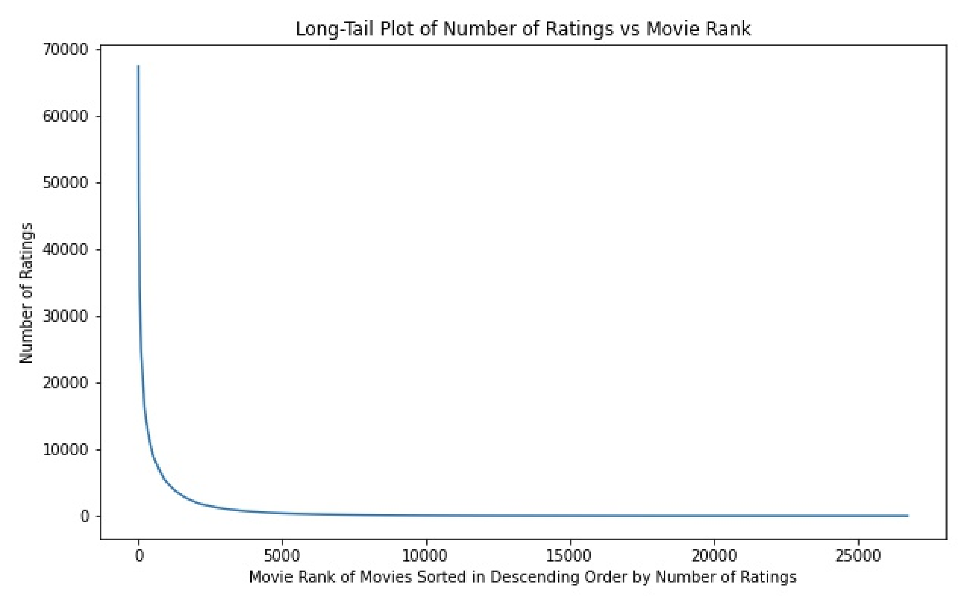
Figure 3-1. Zipfian Distribution of Movierank ratings

At first glance this behavior is obvious and stark, but is it a problem? Let’s assume our recommender will be built as a user-based CF model–as alluded to in Chapter 2–then how might these distributions effect the recommender?

We will consider the distributional ramifications of the above phenomenon. Let the probability mass function be described by the simple Zipf’s law:

for $M$ number of tokens in the corpus (in the above examples number of movies), $k$ is the rank of a token when sorted by number of occurrences.

Let’s consider users $A$ and $B$, with $N_A=\left|{ℐ}_A\right|$ and $N_B=\left|{ℐ}_B\right|$ ratings respectively. Observe that the probability of $V_i$, the $i$‘th most popular video, appearing in ${ℐ}_X$ for some user $X$ is given by:

and thus the joint probability of an item appearing in two user’s ratings is:

In words, the probability of two users sharing an item in their rating sets drops off with the square of its popularity rank.

This becomes important when one also considers that our, yet unstated, definition of user-based collaborative filtering is based on similarity in user’s ratings sets. This similarity is the number of jointly rated items by two users, divided by the total number of items rated by either.

Taking this definition we can, for example, compute the similarity score for one shared item amongst $A$ and $B$:

and the average similarity score of two users is generalized to:

via repeated application of the above observation.

These combinatorial formulas indicate not only the relevance of the Zipfian in our algorithms, but we see an almost direct effect on the output of scores. Consider the experiment from (Wang, Wang, and Zhang 2019) on the LastFM dataset. LastFM is a music listening tracker for users to keep track of all the songs they listen to; for LastFM users, the authors demonstrate average similarity scores for pairs of users, and they find this Matthew Effect persists into the similarity matrix:

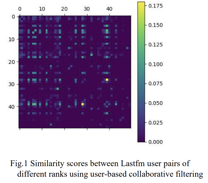
Figure 3-2. Matthew Effect as seen on the LastFM dataset

TODO: Remake this histogram

Observe the radical difference between “hot” cells and all of the others. While these results might seem scary, we’ll consider later some diversity-aware loss functions that we can mitigate some of this. A simpler way is to use downstream sampling methods; which we will discuss as part of our explore-exploit algorithms. Finally, the Matthew Effect is only the first of two major impacts of this Zipfian–let’s turn our attention to the second.

Sparsity

We must now reckon with sparsity. As the ratings skew more and more towards the most popular items, the least popular items are starved for data and recommendations, which is called Data Sparsity. This connects to the linear algebraic definition of sparsity: mostly zeros or not populated elements in a vector. When you consider again our user-item matrix less popular items constitute columns with very few entries–these are sparse vectors. Similarly, at scale we see that the Matthew effect pushes more and more of the total ratings into certain columns, and the matrix becomes sparse in the traditional mathematical sense. For this reason, sparsity is an extremely well known challenge for recommendation systems.

Like above, let’s consider the implication on our collaborative filtering algorithms from these sparse ratings. Again observe that the probability of $V_i$, the $i$‘th most popular item, appearing in ${ℐ}_X$ for some user $X$ is given by:

then

is the expected number of other users which click the $i$‘th most popular item, so summing over all $i$ yields the total number of other users that will share a rating with $X$:

Again, as we pull back to the overall trends, we observe this sparsity sneaking into the actual computations for our collaborative filtering algorithms, consider the trend of users of different ranks, and how much their rankings are used to collaborate in other user’s rankings:

Figure 3-3. User similarity counts for LastFM dataset

We see that this is an important result to always beware–sparsity pushes emphasis onto the most popular users, and has the risk of making your recommender myopic.

User Similarity for Collaborative filtering

In mathematics, it’s very common to hear discussion of distances–even back to the Pythagorean theorem, we are taught to think of relationships between points as distances or dissimilarity. Indeed, this fundamental idea is canonized in mathematics as part of the definition of a metric:

In machine learning; we often instead concern ourselves with the notion of similarity–an extremely related topic. In many cases, one can directly pass back and forth between similarity and dissimilarity; when $d:X\times X\to [0,1]\subset ℝ$ is a dissimilarity function, then we often define:

This may seem like a needlessly precise statement, but in fact we’ll see that there are a (variety of options for how to frame similarity. Furthermore, sometimes we even formulate similarity measures where the associated distance measure does not establish a metric on the set of objects. These so-called pseudo-spaces can still be incredibly important, and we’ll see where they come up in the later section on latent spaces.

In the literature, you’ll find a very common practice of papers starting by introducing a new similarity measure, and then training a model you’ve seen before on the new similarity measure. As we’ll see, choices in how you choose to relate objects(users, items, features, etc.) can have a large effect on what your algorithms learn.

For now, let’s laser in on some specific similarity measures. Consider a classic ML problem of clustering; we have a space (usually ${ℝ}^n$) in which our data is represented and we are asked to partition our data into sub-collections of the population and assign these collections names. Frequently, these collections are intended to capture some meaning, or at the very least be useful for summarizing the collection elements’ features. When you do that clustering, you frequently are considering points near to one another in that space. Further, if you’re given a new observation, and asked to assign it to a collection as an inference task you normally compute the new observation’s nearest neighbors. This could be the k-nearest neighbors, or simply the nearest neighbor amongst cluster centers; either way, your task is to use the notion of similarity to associate–and thus classify. In collaborative filtering, this same notion is used to relate a user for whom you wish to make recommendations, to those you already have data from.

So how may we define similarity for our users in collaborative filtering? They’re not obviously in the same space, so our usual tools seem to be lacking.

Explore–exploit as a RecSys

So far we saw two ideas, slightly in tension with one another:

1. The MPIR, a simple easy to understand recommender

2. The Matthew effect in recommendation systems, and it’s runaway behavior in distributions of ratings

By now, it’s likely that you realize that the MPIR will amplify the Matthew effect, and that the Matthew effect will drive the MPIR to the Trivial recommender in the limit. This is the classic difficulty of maximizing a loss function with no randomization–it very quickly settles into a modal state.

This problem–and many others like it–encourage some modification to the algorithm to prevent this failure mode, and continue to expose the algorithm and users to other options. The basic strategy for explore-exploit schemes, or multi-armed bandits as they’re called, is to take not only the outcome-maximizing recommendation, but also a collection of alternative variants, and randomly determine which to use as response.

Taking a step back: given a collection of variant recommendations, or arms, $A$, for which the outcome of each recommendation is $y_t$, and we have a prior reward function $R\left(y_t\right)$. The bandit–called an agent in this literature–would like to maximize $R\left(y_t\right)$, but the agent doesn’t know the distribution of the outcomes $Y_{a\in A}$. The agent thus assumes some prior distributions for $Y_{a\in A}$, and then collects data to update those distributions; after sufficient observations, the agent can estimate the expected values of each distribution, ${\mu }_{a\in A}=?\left(ℛ\left(Y_a\right)\right)$. If the agent was able to confidently estimate these reward values, the recommendation problem would be solved: at inference, the agent would simply estimate the reward values for all variants for the user, and select the reward-optimizing arm. This is of course ridiculous in totality, but the basic idea is useful nonetheless: hold prior assumptions about what will be greatest expected reward, and explore alternatives with some frequency to continue to update the distributions and refine your estimators.

Even when not explicitly using a multi-armed bandit, this insight is a powerful and useful framework for understanding the goal of a Recsys. Utilizing the ideas of prior estimates for good recommendations, and exploring other options to gain signal is a core idea we’ll see recurring. Let’s see one practicality of this approach.

from jax import random
key = random.PRNGKey(0)


def get_item_popularities() -> Optional[Dict[str, int]]:
    ...
        # Dict of pairs: (item-identifier, count item chosen)
        return item_choice_counts
    return None

def get_most_popular_recs_ep_greedy(
    max_num_recs: int,
    epsilon: float
) -> Optional[List[str]]:
    assert epsilon<1.0
    assert epsilon>0

    items_popularity_dict = get_item_popularities() # type: Optional[Dict[str, int]]
    if items_popularity_dict:
        sorted_items = sorted(
            items_popularity_dict.items(),
            key=lambda item: item[1]),
            reverse=True,
        )
        top_items = [i[0] for i in sorted_items]
        recommendations = []
        for i in range(max_num_recs): # we wish to return max_num_recs
            if random.uniform(key)>epsilon: # if greater than epsilon, exploit
                recommendations.append(top_items.pop(0))
            else: # otherwise, explore
                explore_choice = random.randint(1,len(top_items))
                recommendations.append(top_items.pop(explore_choice))
        return recommendations

    return None

The NLP-RecSys relationship

Let’s utilize some intuition from a different area of Machine Learning, Natural Language Processing. One of the fundamental models in NLP is word2vec; a sequence–based model for language understanding that utilizes the words which co-occur in sentences together.

For skipgram-word2vec, the model takes sentences of words, and attempts to learn the implicit meaning of words via their co-occurrence relationships with other words in those sentences. Each pair of co-occurring words, constitutes a sample that is 1-hot encoded and sent into a vocabulary-sized layer of neurons, with a bottleneck layer, and a vocabulary-sized output layer for probabilities that words will occur.

Via this network, we reduce the size of our representation to the bottleneck dimension, and thus find a smaller dimensional representation of all our words than the original corpus-sized 1-hot embedding. The thinking is that similarity of words can now be computed via vector similarity in this new representation space.

Why is this related to recommendation systems? Well, because if we take the ordered sequence of user-item interactions, e.g. the sequence of movies a user has rated, you can utilize the same idea from word2vec to find item similarity instead of word similarity. In this analogy, the user history is the sentence.

Previously, using our collaborative filtering similarity, we decided that similar users, can help inform what a good recommendation for a user should be. In this model we instead are finding item-item similarity, so instead we assume that items similar to those a user previously liked, they will also like.