Latent Spaces

We are already familiar with feature spaces, which are usually categorical or vector-valued direct representations of the data. This can be the raw red, green, and blue values of an image, counts of items in a histogram, or attributes of an object like length, width, and height. Latent features on the other hand do not represent any specific real value feature of the items, but are initialized randomly and then learned to suit a task. The GloVe embeddings we discussed earlier were one such example of a latent vector that was learned to represent the log-count of words. Here we will cover more ways to generate these latent features or embeddings.

One of the reasons latent spaces are so popular is that they are usually lower in dimension than the features they represent. For example, if the User-Item rating matrix or interaction matrix (where the matrix entries are 1 if a User has interacted with an item) is NxM dimensional, then factorizing the matrix into latent factors of NxK and KxM where K is much smaller then N or M is an approximation the missing entries – this is because we’re relaxing the factorization. K is being smaller than N or M is usually called an information bottleneck. That is, we are forcing the matrix to be made up of a much smaller matrix. This means the machine learning model has to make up missing entries, which might be good for recommender systems. As long as Users have interacted with enough similar items, by forcing the system to have a lot less capacity in terms of degrees of freedom, then it can completely reconstruct the matrix, and the missing entries tend to get filled by similar items.

Let’s see what happens, for example, when we factor a user item matrix of 4x4 into a 4x2 and a 2x4 vector using Singular Value Decomposition (SVD).

We are supplying a matrix whose rows are users and columns are items. For example, row 0 is [1, 0, 0, 1] which means user 0 has selected item 0 and item 3. These can be ratings or purchases. Now let’s look at some code:

import numpy as np

a = np.array([
    [1, 0, 0 ,1],
    [1, 0, 0 ,0],
    [0, 1, 1, 0],
    [0, 1, 0, 0]]
)

u, s, v = np.linalg.svd(a, full_matrices=False)

# Set the last two eigenvalues to 0.
s[2:4] = 0
print(s)
b = np.dot(u * s, v)
print(b)

# These are the eigenvalues with the smallest two set to 0.
s = [1.61803399 1.61803399 0.         0.        ]

# This is the newly reconstructed matrix.
b = [[1.17082039 0.         0.         0.7236068 ]
 [0.7236068  0.         0.         0.4472136 ]
 [0.         1.17082039 0.7236068  0.        ]
 [0.         0.7236068  0.4472136  0.        ]]

Notice that the user in row 1 now has a score for an item in column 3, and the user in row 3 now has a positive score in for the item column 2. This phenomenon is generally known as matrix completion, and is a good property for recommender systems to have because now we get to recommend new items to users. The general method of forcing the machine learning to go through a bottleneck that is smaller than the size of the matrix that it is trying to reconstruct is known as a low-rank approximation because the rank of the approximation is 2 but the rank of the original user-item matrix is 4.

We will cover SVD in more detail later in the chapter, this was just to whet your appetite to how latent spaces are related to recommender systems.

Dot product similarity

In section 1 we introduced similarity measures, but now we return to the dot-product in the context of similarity because of their increased importance in latent-spaces – after all, latent-spaces are build on the assumption that distance is similarity.

The dot product similarity is meaningful in recommendation systems because it provides a geometric interpretation of the relationship between users and items in the latent space (or potentially items and items, users and users, etc.). In the context of recommendation systems, the dot product can be seen as a projection of one vector onto another, indicating the degree of similarity or alignment between the user’s preferences and the item’s characteristics.

To understand the geometric significance of the dot product, consider two vectors, u and p, representing the user and the product in the latent space, respectively. The dot product of these two vectors can be defined as:

where ||u|| and ||p|| represent the magnitudes of the user and product vectors, and θ is the angle between them. The dot product is thus a measure of the projection of one vector onto another, which is scaled by the magnitudes of both vectors.

The cosine similarity, which is another popular similarity measure in recommendation systems, is derived directly from the dot product:

The cosine similarity ranges from -1 to 1, where -1 indicates completely dissimilar preferences and characteristics. 0 indicates no similarity, and 1 indicates perfect alignment between the user’s preferences and the product’s characteristics. In the context of recommendation systems, cosine similarity provides a normalized measure of similarity that is invariant to the magnitudes of the user and product vectors. Note that the choice of using cosine similarity vs L2 distance depends on the type of embeddings you’re using, and how you optimize the computations. Often in practice the only important thing is the relative values.

The geometric interpretation of the dot product (and cosine similarity) in recommendation systems is that it captures the alignment between user preferences and product characteristics. If the angle between the user and product vectors is small, it means that the user’s preferences align well with the product’s characteristics, leading to a higher similarity score. Conversely, if the angle is large, the user’s preferences and product’s characteristics are dissimilar, resulting in a lower similarity score. By projecting user and item vectors onto each other, the dot product similarity can capture the degree of alignment between user preferences and item characteristics, allowing the recommendation system to identify items that are most likely to be relevant and appealing to the user.

Anecdotally, the dot product seems to capture popularity as very long vectors tend to be easy to project on anything that isn’t completely perpendicular or pointing away from them. As a result, there is a tradeoff between frequently recommending popular items with a large vector length from longer tail items that have smaller angular difference with cosine distance.

Figure 10-1. Cosine vs Dot product similarity

Figure 10-1 Considers two vectors, a and b. With Cosine similarity the vectors are unit length so the angle is just the measure of similarity. However, with dot product, a very long vector like c might be considered more similar to a than b even though the angle beween a and b is smaller due to the longer length of c. These long vectors tend to be very popular items that co-occur with many other items.

Co-occurrence models

In our Wikipedia co-occurrences examples, we determined that the co-occurrence structure between two items could be used to generate measures of similarity. We covered how pointwise mutual information can take the counts of co-occurrence, and make recommendations based on very high mutual information between an item in cart, and others.

When we discussed PMI, we found that it was not a distance metric, but still had some important similarity measures based on co-occurrence. Let’s return to this.

Recall from earlier that PMI is defined:

Now let’s consider the discrete co-occurrence distribution $C{D}_{x_i}$ defined as the collection of co-occurrences over all other $x_j$:

where $j\in 1...N$ and $N$ is the total number of items. This represents the co-occurrence histogram between $x_i$ and all other items. By introducing this discrete distribution we can utilize another tool: the Hellinger Distance.

There are a few different ways to measure distributional distance, each with different advantages. For our discussion we will not go deeply into the differences, and stick to the simplest but most appropriate. Hellinger distance is defined as:

$P=p_i〉$ and $Q=q_i〉$ two probability density vectors. In our setting these $P$ and $Q$ can be $C{D}_{x_i}$ and $C{D}_{x_j}$.

The motivation of this process is that we now have a proper distance between items purely based on co-occurrences. We can use any dimension transformation or reduction on this geometry. Later we will see dimension reduction techniques that can utilize an arbitrary distance matrix and reduce the space to a lower dimensional embedding that approximates it.

Reducing the rank of a recommender problem

We’ve seen how, as the number of items and users grows, we very rapidly increase the dimensionality of our recommender problem. Because we’re representing each item and user as a column or vector, this scales like $n^2$. One way to push back against this difficulty is by rank-reduction; recall our previous discussions about rank reduction via factorization.

Like many integers, many matrices can be factored into smaller matrices ; for integers smaller means of smaller value, for matrices smaller means of smaller dimensions. When we factor an $N\times M$ matrix, we will be looking for two matrices $U_{N\times d}$ and $V_{d\times M}$; note that for matrices when you multiply them together they must share a dimension, and that dimension is eliminated leaving the other two. Here, we’ll consider matrix factorizations when $d\le N$ and $d\le M$. By factorizing a matrix, we ask for two matrices which together equal, or approximate, the original matrix:

We seek a small value for $d$ to reduce the number of latent dimensions. As you may have already noticed, each of the matrices $U_{n\times d}$ and $V_{d\times m}$ will correspond to rows or columns of the original ratings matrix. However, they’re expressed in fewer dimensions. This utilizes the idea of a low-dimensional latent space. Intuitively, a latent space seeks to represent the same relationships as the full $n\times m$ dimensional relationships in two sets of relationships: items vs. latent features and users vs. latent features.

These methods are also very popular in other kinds of machine learning, but for our case, we’ll primarily be looking at factorizing ratings or interaction matrices.

There are frequently a few challenges to overcome when considering matrix factorization:

1. the matrix you wish to factor is sparse and often non-negative and/or binary.

2. the number of non-zero elements in each item vector can vary wildly like we saw in the Matthew effect.

3. factorizing matrices is cubic in complexity.

4. SVD and other full rank methods don’t work without imputation, which itself is complicated.

We’ll address these with some alternative optimization methods.

Regularized Matrix Factorization Implementation

So far we’ve written a lot of math symbols, but all of those symbols have allowed us to arrive at a model which is extremely powerful. Regularized Matrix Factorization is an effective model for medium sized recommender problems. This model type is still in prod for many serious businesses. One classic issue with Matrix Factorization (MF) implementations is performance, but because we’re working in JAX which has extremely native GPU support, our implementation can actually be much more compact than what you may find in something like a pyTorch example.

Let’s work through how this model would look to predict ratings for a user-item matrix via this doubly regularized model with Gramians.

First we’ll do the simple setup. This will assume your ratings matrix is already on wandb:

import jax
import jax.numpy as jnp
import numpy as np
import pandas as pd
import os, json, wandb, math

from jax import grad, jit
from jax import random
from jax.experimental import sparse

key = random.PRNGKey(0)

wandb.login()
run = wandb.init(
    # Set entity to specify your username or team name
    entity="wandb-un",
    # Set the project where this run will be logged
    project="jax-mf",
    # associate the runs to the right dataset
    config={
      "dataset": "MF-Dataset",
    }
)

# note that we assume the dataset is a ratings table stored in wandb
artifact = run.use_artifact('stored-dataset:latest')
ratings_artifact = artifact.download()
ratings_artifact_blob = json.load(
    open(
        os.path.join(
            ratings_artifact,
            'ratings.table.json'
        )
    )
)

ratings_artifact_blob.keys()
# ['_type', 'column_types', 'columns', 'data', 'ncols', 'nrows']

ratings = pd.DataFrame( # user_id, item_id, rating, unix_timestamp
    data=ratings_artifact_blob['data'],
    columns=ratings_artifact_blob['columns']
)

def start_pipeline(df):
    return df.copy()

def column_as_type(df, column: str, cast_type):
    df[column] = df[column].astype(cast_type)
    return df

def rename_column_value(df, target_column, prior_val, post_val):
    df[target_column] = df[target_column].replace({prior_val: post_val})
    return df

def split_dataframe(df, holdout_fraction=0.1):
    """Splits a DataFrame into training and test sets.
    Args:
      df: a dataframe.
      holdout_fraction: fraction of dataframe rows to use in the test set.
    Returns:
      train: dataframe for training
      test: dataframe for testing
    """
    test = df.sample(frac=holdout_fraction, replace=False)
    train = df[~df.index.isin(test.index)]
    return train, test

all_rat = (ratings
    .pipe(start_pipeline)
    .pipe(column_as_type, column='user_id', cast_type=int)
    .pipe(column_as_type, column='item_id', cast_type=int)
)

def ratings_to_sparse_array(ratings_df, user_dim, item_dim):
    indices = (np.array(ratings_df['user_id']), np.array(ratings_df['item_id']))
    values = jnp.array(ratings_df['rating'])

    return {
        'indices': indices,
        'values': values,
        'shape': [user_dim, item_dim]
    }

def random_normal(pr_key, shape, mu=0, sigma=1, ):
    return (mu + sigma * random.normal(pr_key, shape=shape))

x = random_normal(
    pr_key = random.PRNGKey(1701),
    shape=(10000,),
    mu = 1.0,
    sigma = 3.0,
) # these hyperparameters are pretty meaningless

def sp_mse_loss(A, params):
    U, V = params['users'], params['items']
    rows, columns = A['indices']
    estimator = -(U @ V.T)[(rows, columns)]
    square_err = jax.tree_map(
        lambda x: x**2,
        A['values']+estimator
    )
    return jnp.mean(square_err)

omse_loss = jit(sp_mse_loss)

Note that we’ve had to implement our own loss function here. This is a relatively straightforward MSE loss but it’s taking advantage of the sparse nature of our matrix. You may notice in the above that we’ve converted the matrix to a sparse representation, so it’s important that our loss function can not only take advantage of that representation, but that it’s written to utilize the JAX device arrays and mapping/jitting.

Is that loss function really right?

If you’re curious about this loss function which appeared like magic, I understand. During the writing of this book I was extremely uncertain what the best implementation of this loss function that leverages JAX would look like. There’s actually many reasonable approaches to this kind of optimization. To that end, I wrote a public experiment to benchmark several different approaches here.

Next, we need to build some model objects to handle our MF state as we train. This code, while essentially mostly template code, will set us up well to feed the model into a training loop in a relatively memory efficient way. This model was trained on 100M entries for a few thousand epochs on a Macbook Pro in less than a day.

class CFModel(object):
    """Simple class that represents a collaborative filtering model"""
    def __init__(
          self,
          metrics: dict,
          embeddings: dict,
          ground_truth: dict,
          embeddings_parameters: dict,
          prng_key=None
    ):
        """Initializes a CFModel.
        Args:
        """
        self._metrics = metrics
        self._embeddings = embeddings
        self._ground_truth = ground_truth
        self._embeddings_parameters = embeddings_parameters

        if prng_key is None:
            prng_key = random.PRNGKey(0)
        self._prng_key = prng_key


    @property
    def embeddings(self):
        """The embeddings dictionary."""
        return self._embeddings

    @embeddings.setter
    def embeddings(self, value):
        self._embeddings = value

    @property
    def metrics(self):
        """The metrics dictionary."""
        return self._metrics

    @property
    def ground_truth(self):
        """The train/test dictionary."""
        return self._ground_truth

    def reset_embeddings(self):
        """Clear out embeddings state."""

        prng_key1, prng_key2 = random.split(self._prng_key, 2)

        self._embeddings['users'] = random_normal(
            prng_key1,
            [
              self._embeddings_parameters['user_dim'],
              self._embeddings_parameters['embedding_dim']
            ],
            mu=0,
            sigma=self._embeddings_parameters['init_stddev'],
        )
        self._embeddings['items'] = random_normal(
            prng_key2,
            [
              self._embeddings_parameters['item_dim'],
              self._embeddings_parameters['embedding_dim']],
            mu=0,
            sigma=self._embeddings_parameters['init_stddev'],
        )

def model_constructor(
    ratings_df,
    user_dim,
    item_dim,
    embedding_dim=3,
    init_stddev=1.,
    holdout_fraction=0.2,
    prng_key=None,
    train_set=None,
    test_set=None,
):
    if prng_key is None:
      prng_key = random.PRNGKey(0)

    prng_key1, prng_key2 = random.split(prng_key, 2)

    if (train_set is None) and (test_set is None):
        train, test = (ratings_df
            .pipe(start_pipeline)
            .pipe(split_dataframe, holdout_fraction=holdout_fraction)
        )

        A_train = (train
            .pipe(start_pipeline)
            .pipe(ratings_to_sparse_array, user_dim=user_dim, item_dim=item_dim)
        )
        A_test = (test
            .pipe(start_pipeline)
            .pipe(ratings_to_sparse_array, user_dim=user_dim, item_dim=item_dim)
        )
    elif (train_set is None) ^ (test_set is None):
        raise('Must send train and test if sending one')
    else:
        A_train, A_test = train_set, test_set

    U = random_normal(
        prng_key1,
        [user_dim, embedding_dim],
        mu=0,
        sigma=init_stddev,
    )
    V = random_normal(
        prng_key2,
        [item_dim, embedding_dim],
        mu=0,
        sigma=init_stddev,
    )


    train_loss = omse_loss(A_train, {'users': U, 'items': V})
    test_loss = omse_loss(A_test, {'users': U, 'items': V})

    metrics = {
        'train_error': train_loss,
        'test_error': test_loss
    }
    embeddings = {'users': U, 'items': V}
    ground_truth = {
        "A_train": A_train,
        "A_test": A_test
    }
    return CFModel(
        metrics=metrics,
        embeddings=embeddings,
        ground_truth=ground_truth,
        embeddings_parameters={
            'user_dim': user_dim,
            'item_dim': item_dim,
            'embedding_dim': embedding_dim,
            'init_stddev': init_stddev,
        },
        prng_key=prng_key,
    )

mf_model = model_constructor(all_rat, user_count, item_count)

We should also set this up to log nicely to wandb so it’s easy to understand what is happening during training:

def train():
  run_config = { # These will be hyperparameters we will tune via wandb
      'emb_dim': 10, # Latent dimension
      'prior_std': 0.1, # Std dev around 0 for weights initialization
      'alpha': 1.0, # Learning rate
      'steps': 1500, # Number of training steps
  }

  with wandb.init() as run:
    run_config.update(run.config)
    model_object = model_constructor(
        ratings_df=all_rat,
        user_dim=user_count,
        item_dim=item_count,
        embedding_dim=run_config['emb_dim'],
        init_stddev=run_config['prior_std'],
        prng_key=random.PRNGKey(0),
        train_set=mf_model.ground_truth['A_train'],
        test_set=mf_model.ground_truth['A_test']
    )
    model_object.reset_embeddings() # Ensure we are starting from priors
    alpha, steps = run_config['alpha'], run_config['steps']
    print(run_config)
    grad_fn = jax.value_and_grad(omse_loss, 1)
    for i in range(steps):
      # We perform one gradient update
      loss_val, grads = grad_fn(
          model_object.ground_truth['A_train'],
          model_object.embeddings
      )
      model_object.embeddings = jax.tree_multimap(
          lambda p, g: p - alpha * g,
          # Basic update rule; JAX handles broadcasting for us
          model_object.embeddings,
          grads
      )
      if i % 1000 == 0: # Most output in wandb; little bit of logging
        print(f'Loss step {i}: ', loss_val)
        print(f"""Test loss: {
            omse_loss(
                model_object.ground_truth['A_train'],
                model_object.embeddings
            )}""")

      wandb.log({
          "Train omse": loss_val,
          "Test omse": omse_loss(
              model_object.ground_truth['A_test'],
              model_object.embeddings
           )
      })

Note that this is using the tree_multimap to handle broadcasting our update rule, and we’re using the jitted loss from before in the omse_loss call. Also, we’re calling value_and_grad so we can log the loss to wandb as we go. This is a common trick you’ll see for efficiently doing both without a callback.

You can finish this off and start the training with a sweep:

sweep_config = {
    "name" : "mf-test-sweep",
    "method" : "random",
    "parameters" : {
        "steps" : {
            "min": 1000,
            "max": 3000,
        },
        "alpha" :{
            "min": 0.6,
            "max": 1.75
        },
        "emb_dim" :{
            "min": 3,
            "max": 10
        },
        "prior_std" :{
            "min": .5,
            "max": 2.0
        },
    },
    "metric" : {
        'name': 'Test omse',
        'goal': 'minimize'
    }
}

sweep_id = wandb.sweep(sweep_config, project="jax-mf", entity="wandb-un")

wandb.init()
train()

count = 50
wandb.agent(sweep_id, function=train, count=count)

In this case the hyperparameter optimization is over our hyperparameters like embedding dimension and the priors (randomized matrices). Up until now, we have trained some MF models on our ratings matrix. Let’s now add regularlization and cross-validation.

Translating the math equations above directly into code:

def ell_two_regularlization_term(params, dimensions):
    U, V = params['users'], params['items']
    N, M = dimensions['users'], dimensions['items']
    user_sq = jnp.multiply(U, U)
    item_sq = jnp.multiply(V, V)
    return (jnp.sum(user_sq)/N + jnp.sum(item_sq)/M)

l2_loss = jit(ell_two_regularlization_term)

def gramian_regularization_term(params, dimensions):
    U, V = params['users'], params['items']
    N, M = dimensions['users'], dimensions['items']
    gr_user = U.T @ U
    gr_item = V.T @ V
    gr_square = jnp.multiply(gr_user, gr_item)
    return (jnp.sum(gr_square)/(N*M))

gr_loss = jit(gramian_regularization_term)

def regularized_omse(A, params, dimensions, hyperparams):
  lr, lg = hyperparams['ell_2'], hyperparams['gram']
  losses = {
      'omse': sp_mse_loss(A, params),
      'l2_loss': l2_loss(params, dimensions),
      'gr_loss': gr_loss(params, dimensions),
  }
  losses.update({
      'total_loss': losses['omse'] + lr*losses['l2_loss'] + lg*losses['gr_loss']
  })
  return losses['total_loss'], losses

reg_loss_observed = jit(regularized_omse)

We won’t dive super deep into learning rate schedulers, but we will do a simple decay:

def lr_decay(
    step_num,
    base_learning_rate,
    decay_pct = 0.5,
    period_length = 100.0
):
    return base_learning_rate * math.pow(
        decay_pct,
        math.floor((1+step_num)/period_length)
    )

Our updated train function will incorporate our new regularlizations – which come with some hyperparameters – and a bit of additional logging setup. This code is making it easy to log our experiment as it trains, and configures the hyperparameters to work with regularlization.

def train_with_reg_loss():
    run_config = { # These will be hyperparameters we will tune via wandb
        'emb_dim': None,
        'prior_std': None,
        'alpha': None, # Learning rate
        'steps': None,
        'ell_2': 1, #l2 regularlization penalization weight
        'gram': 1, #gramian regularlization penalization weight
        'decay_pct': 0.5,
        'period_length': 100.0
    }

    with wandb.init() as run:
        run_config.update(run.config)
        model_object = model_constructor(
            ratings_df=all_rat,
            user_dim=942,
            item_dim=1681,
            embedding_dim=run_config['emb_dim'],
            init_stddev=run_config['prior_std'],
            prng_key=random.PRNGKey(0),
            train_set=mf_model.ground_truth['A_train'],
            test_set=mf_model.ground_truth['A_test']
        )
        model_object.reset_embeddings() # Ensure we start from priors

        alpha, steps = run_config['alpha'], run_config['steps']
        print(run_config)

        grad_fn = jax.value_and_grad(
            reg_loss_observed,
            1,
            has_aux=True
        ) # Tell JAX to expect an aux dict as output

        for i in range(steps):
            (total_loss_val, loss_dict), grads = grad_fn(
                model_object.ground_truth['A_train'],
                model_object.embeddings,
                dimensions={'users': user_count, 'items': item_count},
                hyperparams={
                    'ell_2': run_config['ell_2'],
                    'gram': run_config['gram']
                } # JAX carries our loss dict along for logging
            )


            model_object.embeddings = jax.tree_multimap(
                lambda p, g: p - lr_decay(
                    i,
                    alpha,
                    run_config['decay_pct'],
                    run_config['period_length']
                ) * g, # update with decay
                model_object.embeddings,
                grads
            )
            if i % 1000 == 0:
                print(f'Loss step {i}:')
                print(loss_dict)
                print(f"""Test loss: {
                    omse_loss(model_object.ground_truth['A_test'],
                    model_object.embeddings)}""")

            loss_dict.update( # wandb takes the entire loss dictionary
                {
                    "Test omse": omse_loss(
                        model_object.ground_truth['A_test'],
                        model_object.embeddings
                    ),
                    "learning_rate": lr_decay(i, alpha),
                }
            )
            wandb.log(loss_dict)

 sweep_config = {
    "name" : "mf-HPO-with-reg",
    "method" : "random",
    "parameters" : {
      "steps": {
        "value": 2000
      },
      "alpha" :{
        "min": 0.6,
        "max": 2.25
      },
      "emb_dim" :{
        "min": 15,
        "max": 80
      },
      "prior_std" :{
        "min": .5,
        "max": 2.0
      },
      "ell_2" :{
        "min": .05,
        "max": 0.5
      },
      "gram" :{
        "min": .1,
        "max": .75
      },
      "decay_pct" :{
        "min": .2,
        "max": .8
      },
      "period_length" :{
        "min": 50,
        "max": 500
      }
    },
    "metric" : {
      'name': 'Test omse',
      'goal': 'minimize'
    }
  }

  sweep_id = wandb.sweep(
      sweep_config,
      project="jax-mf",
      entity="wandb-un"
  )

run_config = { # These will be hyperparameters we will tune via wandb
      'emb_dim': 10, # Latent dimension
      'prior_std': 0.1,
      'alpha': 1.0, # Learning rate
      'steps': 1000, # Number of training steps
      'ell_2': 1, #l2 regularlization penalization weight
      'gram': 1, #gramian regularlization penalization weight
      'decay_pct': 0.5,
      'period_length': 100.0
  }

train_with_reg_loss()

The last step is to do this in a way that gives us confidence in the models we’re seeing. Unfortunately, it can be a bit tricky to setup cross-validation for Matrix Factorization problems, so we’ll need to make a few modifications to our data structures.

def sparse_array_concatenate(sparse_array_iterable):
    return {
        'indices': tuple(
            map(
                jnp.concatenate,
                zip(*(x['indices'] for x in sparse_array_iterable)))
            ),
        'values': jnp.concatenate(
            [x['values'] for x in sparse_array_iterable]
        ),
    }

class jax_df_Kfold(object):
    """Simple class that handles Kfold
    splitting of a matrix as a dataframe and stores as sparse jarrays"""
    def __init__(
        self,
        df: pd.DataFrame,
        user_dim: int,
        item_dim: int,
        k: int = 5,
        prng_key=random.PRNGKey(0)
    ):
        self._df = df
        self._num_folds = k
        self._split_idxes = jnp.array_split(
            random.permutation(
                prng_key,
                df.index.to_numpy(),
                axis=0,
                independent=True
            ),
            self._num_folds
        )

        self._fold_arrays = dict()

        for fold_index in range(self._num_folds):
        # let's create sparse jax arrays for each fold piece
            self._fold_arrays[fold_index] = (
                self._df[
                    self._df.index.isin(self._split_idxes[fold_index])
                ].pipe(start_pipeline)
                .pipe(
                    ratings_to_sparse_array,
                    user_dim=user_dim,
                    item_dim=item_dim
                )
            )

    def get_fold(self, fold_index: int):
        assert(self._num_folds > fold_index)
        test = self._fold_arrays[fold_index]
        train = sparse_array_concatenate(
            [v for k,v in self._fold_arrays.items() if k != fold_index]
        )
        return train, test

Each hyperparam setup should yield loss for each fold, so within the wandb.init, we build a model with each fold, thus:

for j in num_folds:
  train, test = folder.get_fold(j)
  model_object_dict[j] = model_constructor(
          ratings_df=all_rat,
          user_dim=user_count,
          item_dim=item_count,
          embedding_dim=run_config['emb_dim'],
          init_stddev=run_config['prior_std'],
          prng_key=random.PRNGKey(0),
          train_set=train,
          test_set=test
      )

At each step, we’d like to not only compute the gradient for the training and evaluate on the test, we’d like to also compute gradients for all folds, eval on all the tests, and produce the relevant errors.

for i in range(steps):
    loss_dict = {"learning_rate": step_decay(i)}
    for j, M in model_object_dict.items():
        (total_loss_val, fold_loss_dict), grads = grad_fn(
            M.ground_truth['A_train'],
            M.embeddings,
            dimensions={'users': 942, 'items': 1681},
            hyperparams={'ell_2': run_config['ell_2'], 'gram': run_config['gram']}
        )

        M.embeddings = jax.tree_multimap(
            lambda p, g: p - step_decay(i) * g,
            M.embeddings,
            grads
        )

Logging should be losses per fold, and the aggregate loss should be the target metric. This is because each fold is an independent optimization of the model parameters, however we wish to see aggregate behavior across the folds.

        fold_loss_dict = {f'{k}_fold-{j}': v for k, v in fold_loss_dict.items()}
        fold_loss_dict.update(
                  {
                      f"Test omse_fold-{j}": omse_loss(
                        M.ground_truth['A_test'],
                        M.embeddings
                      ),
                  }
              )

        loss_dict.update(fold_loss_dict)

    loss_dict.update({
      "Test omse_mean": jnp.mean(
        [v for k,v in loss_dict.items() if k.startswith('Test omse_fold-')]
      )
    })
    wandb.log(loss_dict)

Which we wrap up into one big training method:

def train_with_reg_loss_CV():
    run_config = { # These will be hyperparameters we will tune via wandb
        'emb_dim': None, # Latent dimension
        'prior_std': None,
        # Standard deviation around 0 that our weights are initialized to
        'alpha': None, # Learning rate
        'steps': None, # Number of training steps
        'num_folds': None, # Number of CV Folds
        'ell_2': 1, #hyperparameter for l2 regularlization penalization weight
        'gram': 1, #hyperparameter for gramian regularlization penalization weight
    }

    with wandb.init() as run:
        run_config.update(run.config) # This is how the wandb agent passes along params
        model_object_dict = dict()

        for j in range(run_config['num_folds']):
            train, test = folder.get_fold(j)
            model_object_dict[j] = model_constructor(
                ratings_df=all_rat,
                user_dim=942,
                item_dim=1681,
                embedding_dim=run_config['emb_dim'],
                init_stddev=run_config['prior_std'],
                prng_key=random.PRNGKey(0),
                train_set=train,
                test_set=test
            )
            model_object_dict[j].reset_embeddings()
            # Ensure we are starting from priors

        alpha, steps = run_config['alpha'], run_config['steps']
        print(run_config)

        grad_fn = jax.value_and_grad(reg_loss_observed, 1, has_aux=True)
        # Tell JAX to expect an aux dict as output

        for i in range(steps):
            loss_dict = {
              "learning_rate": lr_decay(
                i,
                alpha,
                decay_pct=.75,
                period_length=250
              )
            }
            for j, M in model_object_dict.items():
            # Iterate through folds

                (total_loss_val, fold_loss_dict), grads = grad_fn(
                # compute gradients for one fold
                    M.ground_truth['A_train'],
                    M.embeddings,
                    dimensions={'users': 942, 'items': 1681},
                    hyperparams={
                      'ell_2': run_config['ell_2'],
                      'gram': run_config['gram']
                    }
                )

                M.embeddings = jax.tree_multimap(
                # update weights for one fold
                    lambda p, g: p - lr_decay(
                      i,
                      alpha,
                      decay_pct=.75,
                      period_length=250
                    ) * g,
                    M.embeddings,
                    grads
                )

                fold_loss_dict = {
                  f'{k}_fold-{j}':
                  v for k, v in fold_loss_dict.items()
                }
                fold_loss_dict.update( # loss calculation within fold
                    {
                        f"Test omse_fold-{j}": omse_loss(
                          M.ground_truth['A_test'],
                          M.embeddings
                        ),
                    }
                )

                loss_dict.update(fold_loss_dict)

            loss_dict.update({ # average loss over all folds
                "Test omse_mean": np.mean(
                    [v for k,v in loss_dict.items() if k.startswith('Test omse_fold-')]
                ),
                "test omse_max": np.max(
                    [v for k,v in loss_dict.items() if k.startswith('Test omse_fold-')]
                ),
                "test omse_min": np.min(
                    [v for k,v in loss_dict.items() if k.startswith('Test omse_fold-')]
                )
            })
            wandb.log(loss_dict)

            if i % 1000 == 0: # Most output in wandb; little bit of logging to stdout
                print(f'Loss step {i}:')
                print(loss_dict)

and our final sweeps config:

sweep_config = {
    "name" : "mf-HPO-CV",
    "method" : "random",
    "parameters" : {
      "steps": {
        "value": 2000
      },
      "num_folds": {
        "value": 5
      },
      "alpha" :{
        "min": 2.0,
        "max": 3.0
      },
      "emb_dim" :{
        "min": 15,
        "max": 70
      },
      "prior_std" :{
        "min": .75,
        "max": 1.0
      },
      "ell_2" :{
        "min": .05,
        "max": 0.5
      },
      "gram" :{
        "min": .1,
        "max": .6
      },
    },
    "metric" : {
      'name': 'Test omse_mean',
      'goal': 'minimize'
    }
  }

  sweep_id = wandb.sweep(sweep_config, project="jax-mf", entity="wandb-un")


wandb.agent(sweep_id, function=train_with_reg_loss_CV, count=count)

That may seem like a lot of setup, but we’ve really acheived a lot here. We’ve initialized the model to optimize the two matrix factors, while simultaneously keeping the matrix elements small, and keeping the gramians small also.

Which brings us to our lovely images.

Output from HPO MF

Let’s have a quick look at what what the prior work has produced. First, we see (Figure 10-3) that our primary loss function, OMSE, is rapidly decreasing. This is great, but we should take a deeper look.

Figure 10-3. The loss during training

Let’s also have a quick check that our regularization parameters (Figure 10-4) are converging, and we see that our l2 regularization could probably still decrease if we were to continue for more epochs.

Figure 10-4. Regularization Params

We’d like to see our cross-validation layed out by fold and corresponding loss (Figure 10-5). This kind of plot is called a parallel coordinates chart; it’s lines correspond to different runs which are in correspondance with different choices of parameters, and it’s vertical axes are different metrics. The far right heatmap axis corresponds to the overall total loss which we’re trying to minimize. In this case we alternate test loss on a fold and total loss on that fold. Lower numbers are better, and we hope to see individual lines consistent across their loss per fold (otherwise we may have a skewed dataset). We see that choices of hyper-parameters can interact with fold behavior, but in all of the low loss scenarios (at the bottom), we see a very high correlation between performance on different folds (the vertical axes in the plot).

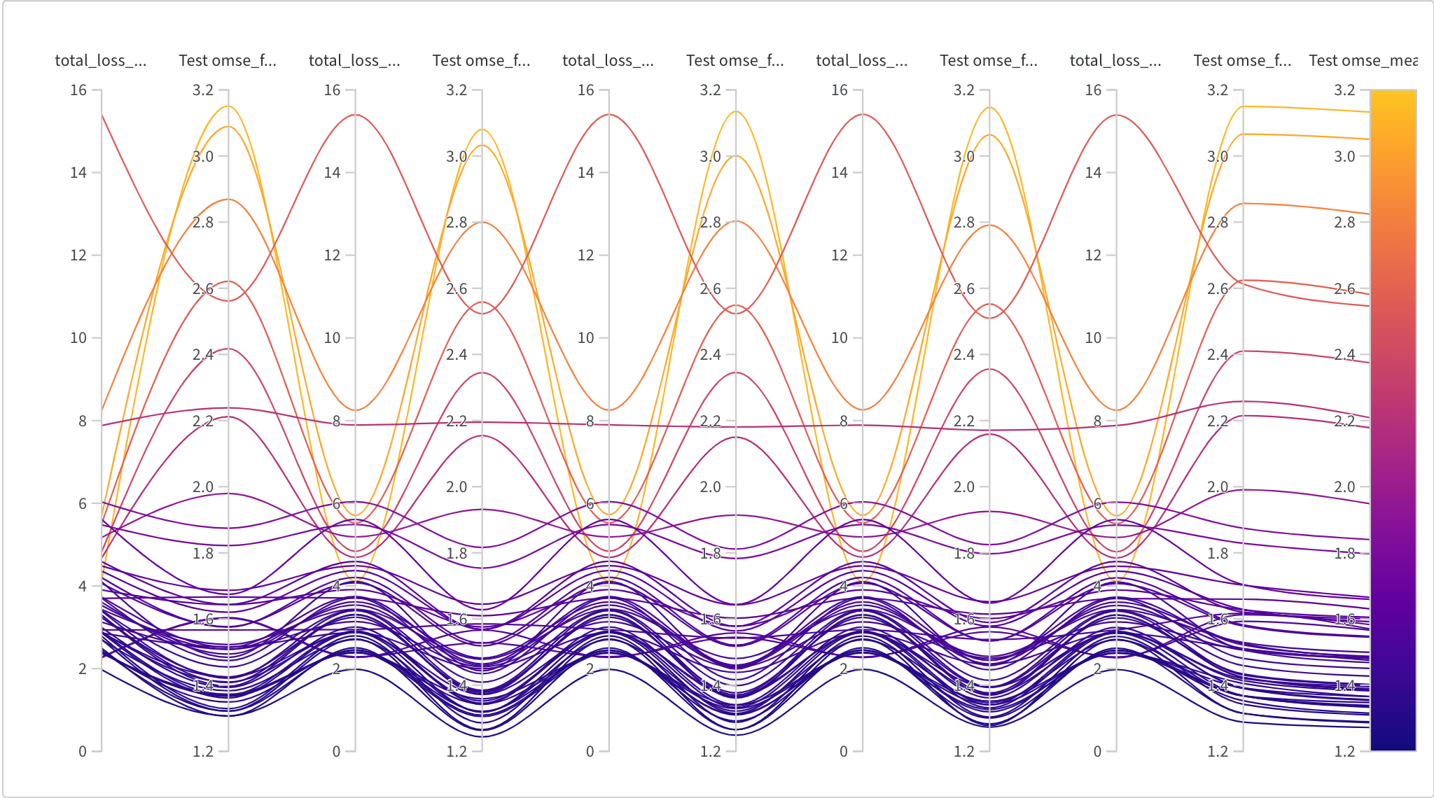
Figure 10-5. The loss during training

Next up, which choices of hyper-parameters have a strong effect on performance? In Figure 10-6 we have another parallel coordinates plot where the verticle axes correspond to different hyperparamaters. Generally we’re looking for which domains on the vertical axes correspond to low loss on the far right heatmap. We see that some of our hyperparameters like priors distribution and somewhat surprisingly ell_2 have virtually no effect. However, small embedding dimension and small gramian weight definitely do. A larger alpha also seems to correlate well with good performance.

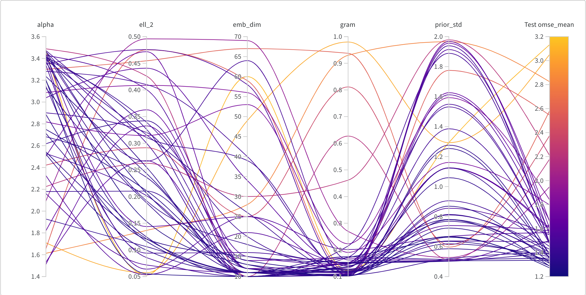
Figure 10-6. The loss during training

Finally, we see that as we do a Bayesian hyperparameter search, we really do improve our performance over time. The plot Figure 10-7, is a Pareto plot, where each dot in the scatter plot represents on run, and left to right is a time axis. The vertical axis is overall total loss, so lower is better, and it means that generally we’re converging towards better performance. The line inscribed along the bottom of the convex hull of the scatter points is the Pareto Frontier or “the best performance at that x value”. Since this is a time-series Pareto plot, this merely tracks the best performance in time. You may be wondering how and why we’re able to converge to better loss values in time. This is because we’ve conducted a Bayesian hyperparameter search, which means we select our hyperparameters from a independent Gaussians, and we update our priors for each parameter based on performance of previous runs; for an introduction to this method, this blog post covers it well. In a real setting, we’d see less monotonic behavior in this plot, but we’d be always hoping to improve.

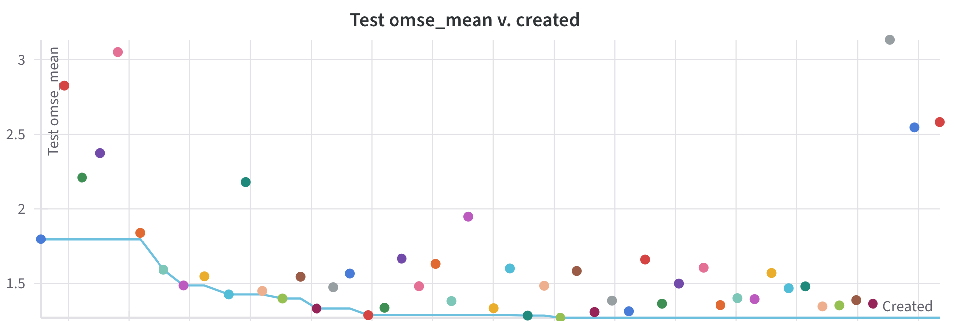
Figure 10-7. The loss during training

Pre-quential validation

If we were to put the above approach into practice, we would need to capture our trained models in a model registry for use in production.

Best practice is to establish a set of explicit evaluations to test a selection of models against. In your basic ML training, you’ve likely been encouraged to think about a validation dataset; these may take a lot of different forms, testing particular subsets of instances or features or even distributed across covariates in a known way.

One useful thing to do for recommendation systems, is to remember that they’re a fundamentally sequential dataset. With this in mind, let’s take another look at our ratings data. Later we will talk more about sequential recommenders, but while we’re talking about validation, it’s useful to mention how to take proper care.

Notice that all of our ratings have an associated timestamp. This means to build a proper validation set, it’s a good idea to take that from the end of our data.

However, you might be wondering: “when are different users active?” and “is it possible that the later timestamps are a biased selection of the ratings”. These are very important questions. To account this, we should do a holdout by user.

A simple way to generate this prequential dataset, a holdout-test dataset where the holdout is a contiguous series temporally after the holdout dataset, is to determine an approximate size you’d like for validation, say 10%, then group by user, then use rejection sampling with the rejection condition not largest timestamp.

Here’s a simple implementation for pandas using rejection sampling. This is not the most computationally efficient implementation, but it will get the job done:

def prequential_validation_set(df, holdout_perc=0.1):
    '''
    We utilize rejection sampling.

    Assign a probability to all observations, if they lie below the
    sample percentage AND they're the most recent still in the set, include.

    Otherwise return them and repeat.
    Each time, take no more than the remaining necessary to fill the count.
    '''
    count = int(len(df)*holdout_perc)
    sample = []
    while count >0:
      df['p'] = np.random.rand(len(df),1) #generate probabilities
      x = list(
          df.loc[~df.index.isin(sample)] # exclude already selected
          .sort_values(['unix_timestamp'], ascending=False) # sort by timestamp desc
          .groupby('user_id').head(1) # only allow the first in each group
          .query("p < @holdout_perc").index # grab the indices
      )
      rnd.shuffle(x) # make sure our previous sorting doesn't bias the users subset
      sample += x[:count] # add observations up to the remaining needed
      count -= len(x[:count]) # decrement the remaining needed

    df.drop(columns=['p'], inplace=True)

    test = df.iloc[sample]
    train = df[~df.index.isin(test.index)]
    return train, test

This is an effective and important validation scheme for inherently sequential datasets.

Dimension Reduction

Dimension reduction techniques are frequently employed in recommendation systems to decrease computational complexity and enhance the accuracy of recommendation algorithms. In this context, the primary concepts of dimension reduction for recommendation systems include:

Matrix factorization: The matrix factorization method decomposes the user-item interaction matrix $(A\in {ℝ}^{(m\times n)})$ into two lower-dimensional matrices, representing the user $(U\in {ℝ}^{(m\times r)})$ and item $(V\in {ℝ}^{(n\times r)})$ latent factors, respectively. This technique can reveal the underlying data structure and offer recommendations based on a user’s previous interactions. Mathematically, matrix factorization can be represented as:

Singular value decomposition (SVD): SVD is a linear algebra technique that decomposes a matrix (A) into three matrices - the left singular vectors (U), the singular values (Σ), and the right singular vectors (V). SVD can be utilized for matrix factorization in recommendation systems, where the user-item interaction matrix is decomposed into a smaller number of latent factors. The mathematical representation of SVD is:

In practice though, rather than using a mathematical library to find the eigenvectors, folks might use the Power Iteration Method to discover the eigenvectors approximately. This method is far more scalable than a full dense SVD solve that is optimized for correctness and dense vectors.

import jax
import jax.numpy as jnp


def power_iteration(a: jnp.ndarray) -> jnp.ndarray:
  """Returns an eigenvector of the matrix a.
  Args:
    a: a n x m matrix
  """
  key = jax.random.PRNGKey(0)
  x = jax.random.normal(key, shape=(a.shape[1], 1))
  for i in range(100):
    x = a @ x
    x = x / jnp.linalg.norm(x)
  return x.T

key = jax.random.PRNGKey(123)
A = jax.random.normal(key, shape=[4, 4])
print(A)
[[ 0.52830553  0.3722206  -1.2219944  -0.10314374]
 [ 1.4722222   0.47889313 -1.2940298   1.0449569 ]
 [ 0.23724185  0.3545859  -0.172465   -1.8011322 ]
 [ 0.4864215   0.08039388 -1.2540827   0.72071517]]
S, _, _ = jnp.linalg.svd(A)
print(S)
[[-0.375782    0.40269807  0.44086716 -0.70870167]
 [-0.753597    0.0482972  -0.65527284  0.01940039]
 [ 0.2040088   0.91405433 -0.15798494  0.31293103]
 [-0.49925917 -0.00250015  0.5927009   0.6320123 ]]
x1 = power_iteration(A)
print(x1.T)
[[-0.35423845]
 [-0.8332922 ]
 [ 0.16189891]
 [-0.39233655]]

Notice that the eigenvector returned by the power iteration is close to the first column of S but not quite. This is because the method is approximate. It relies on the fact that an eigenvector doesn’t change in direction when multiplied by the matrix. So by repeatedly multiplying by the matrix we eventually iterate onto an eigenvector. Also notice that we solved for column eigenvectors instead of the row eigenvectors. In this example, the columns are users and rows are items. It is important to play with transposed matrices as a lot of machine learning involves reshaping and transposing matrices, so getting used to them early is an important skill.

Next, we construct a recommendation for a user by creating a column and then taking the dot product with all the eigenvectors and finding the closest using the dot product. We then find all the highest scoring entries in the eigenvector that the user hasn’t seen and return them as recommendations. So in the example above, if the eigenvector x1 was the closest to the user column, then the best item to recommend would be item 3 because it is the largest component in the eigenvector and thus rated most highly if the user is closest to the eigenvector x_1. Here’s what this looks like in code:

import jax
import jax.numpy as jnp

def recommend_items(eigenvectors: jnp.ndarray, user:jnp.ndarray) -> jnp.ndarray:
  """Returns an ordered list of recommend items for the user.
  Args:
    eigenvectors: a nxm eigenvector matrix
    user: a user vector of size m.
  """
  score_eigenvectors = jnp.matmul(eigenvectors.T, user)
  which_eigenvector = jnp.argmax(score_eigenvectors)
  closest_eigenvector = eigenvectors.T[which_eigenvector]
  scores, items = jax.lax.top_k(closest_eigenvector, 3)
  return scores, items

S = jnp.array(
[[-0.375782,    0.40269807],
 [-0.753597,    0.0482972],
 [ 0.2040088,   0.91405433],
 [-0.49925917, -0.00250015]])
u = jnp.array([-1, -1, 0, 0]).reshape(4, 1)
scores, items = recommend_items(S, u)
print(scores)
[ 0.2040088  -0.375782   -0.49925917]
print(items)
[2 0 3]

In this example, we have a user who has downvoted item 0 and item 1. The closest column eigenvector is therefore column 0. We then select the closest eigenvector to the user and order the entries and recommend item 2 to the user which is the highest scoring entry that the user has not seen.

Two techniques that aim to extract the most relevant features from the user-item interaction matrix and reduce its dimensionality, which can improved performance.

• Principal component analysis (PCA): PCA is a statistical technique that transforms the original high-dimensional data into a lower-dimensional representation while retaining the most important information. PCA can be applied to the user-item interaction matrix to reduce the number of dimensions and improve the computational efficiency of the recommendation algorithm.

• Non-negative matrix factorization (NMF): NMF is a technique that decomposes the non-negative user-item interaction matrix $(A\in {ℝ}^{(m\times n)*+})$ into two non-negative matrices $(W\in {ℝ}^{(m\times r)*+}$ and $H\in {ℝ}^{{(r\times n)}_{+}})$. NMF can be utilized for dimension reduction in recommendation systems, where the latent factors are non-negative and interpretable. The mathematical representation of NMF is: $A\simeq W\times H$.

Matrix factorization techniques can be further extended to incorporate additional information, such as item content or user demographic data, through the use of side information. Side information can be employed to augment the user-item interaction matrix, allowing for more accurate and personalized recommendations.

Furthermore, matrix factorization models can be extended to handle implicit feedback data, where the absence of interaction data is not equivalent to the lack of interest. By incorporating additional regularization terms into the objective function, matrix factorization models can learn a more robust representation of the user-item interaction matrix, leading to better recommendations for implicit feedback scenarios.

Consider a recommendation system that employs matrix factorization to model the user-item interaction matrix. If the system comprises a large number of users and items, the resulting factor matrices can be high-dimensional and computationally expensive to process. However, by using dimension reduction techniques like SVD or PCA, the algorithm can reduce the dimensionality of the factor matrices while preserving the most important information about the user-item interactions. This enables the algorithm to generate more efficient and accurate recommendations, even for new users or items with limited interaction data.

Affinity and p-sale

As we’ve seen, Matrix factorization is a powerful dimension reduction technique that can yield an estimator for the probability of a sale (often shorted to p-sale). In matrix factorization, the goal has been to decompose this the historical data on user behavior and product sales matrix into two lower-dimensional matrices: one that represents user preferences and another that represents product characteristics. Now, let’s convert this MF model into an sale estimator.

Let $R\in {ℝ}^{\left(MxN\right)}$ be the historical data matrix, where m is the number of users and n is the number of products. The matrix factorization aims to find two matrices $U\in {ℝ}^{(M\times d)}$ and $V\in {ℝ}^{(N\times d)}$, where $d$ is the dimensionality of the latent space, such that:

The probability of a sale, or equivalently a read, watch, eat, or click, can be predicted using matrix factorization by first decomposing the historical data matrix into user and product matrices, and then calculating a score that represents the likelihood of a user purchasing a given product. This score can be calculated using the dot product of the corresponding row in the user matrix and column in the product matrix, followed by a logistic function to transform the dot product into a probability score.

Mathematically, the probability of a sale for a user u and a product p can be represented as:

where sigmoid is the logistic function that maps the dot product of the user and product vectors to a probability score between 0 and 1:

and $p^T$ represents the transpose of the product vector. The dot product of the user and product vectors is a measure of the similarity between the user’s preferences and the product’s characteristics, and the logistic function maps this similarity score to a probability score.

The user and product matrices can be trained on the historical data using various matrix factorization algorithms, such as singular value decomposition (SVD), non-negative matrix factorization (NMF), or alternating least squares (ALS). Once the matrices are trained, the dot product and logistic function can be applied to new user-product pairs to predict the probability of a sale. The predicted probabilities can then be used to rank and recommend products to the user.

It’s worth highlight that, since the loss function for ALS is convex (meaning there is a single global minimum) when one fixes either the user or item matrix, the convergence can be very fast. In this method, the user matrix is fixed and the item matrix is solved for. Then the item matrix is fixed and the user matrix is solved for. The method alternates between the two solves and because the loss is convex in this regime, the method converges very quickly.

The dot product of the corresponding row in the user matrix and column in the product matrix represents the affinity score between the user and the product, or how well the user’s preferences match the product’s characteristics. However, this score alone may not be a sufficient predictor of whether the user will actually purchase the product.

The logistic function applied to the dot product in the matrix factorization model transforms the affinity score into a probability score, which represents the likelihood of a sale. This transformation takes into account additional factors beyond just the user’s preferences and the product’s characteristics, such as the overall popularity of the product, the user’s purchasing behavior, and any other relevant external factors. By incorporating these additional factors, matrix factorization is able to better predict the probability of a sale, rather than just an affinity score.

A comparison library (however not in JAX) for computing latent embeddings linearly is Factorization Machines. The formulation for a Factorization Machine is very similar to a GloVe embedding in that it also models the interaction between two vectors but the dot product can be used for regression or binary classification tasks. The method can also be extended to recommend more than two kinds of items beyond user and item.

In summary, matrix factorization produces probabilities of sale instead of just affinity scores by incorporating additional factors beyond just the user’s preferences and the product’s characteristics, and transforming the affinity score into a probability score using a logistic function.

Propensity Weighting for Recommendation System Evaluation

As we’ve seen, recommendation systems are evaluated based on user feedback, which is collected from the deployed recommendation system. However, this data is causally influenced by the deployed system, creating a feedback loop that may bias the evaluation of new models. This feedback loop can lead to confounding variables, making it difficult to distinguish between user preferences and the influence of the deployed system. If this surprises you, let’s consider for a moment what would have to be true for a recommendation system to not causally influence the actions users take and/or the outcomes that result from those actions – that would require things like “the recommendations are completely ignored by the user” and “the system makes recommendations at random”. Propensity weighting can mitigate some of the worst effects of this problem.

The performance of a recommender system depends on many factors, including user-item characteristics, contextual information, and trends, which can affect the quality of the recommendations and the user engagement. However, the influence can be mutual: the user interactions influence the recommender and vice-versa. Evaluating the causal effect of a recommender system on user behavior and satisfaction is therefore a challenging task, as it requires controlling for potential confounding factors, ie things that may affect both the treatment assignment (i.e., the recommendation strategy) and the outcome of interest (i.e., the user’s response to the recommendations).

Causal inference provides a framework for addressing these challenges. In the context of recommender systems, causal inference can help answer questions such as:

• How does the choice of recommendation strategy affect user engagement, such as click-through rates, purchase rates, and satisfaction ratings?

• What is the optimal recommendation strategy for a given user segment, item category, or context?

• What are the long-term effects of a recommendation strategy on user retention, loyalty, and lifetime value?

We’ll round out this chapter by introducing one aspect of causal inference important to recommender systems, based on the concept of propensity score.

Summary

What a whirlwind! Latent spaces are one of the most important aspects of recommendation systems. They are the representations that we use to encode our users and items. Ultimately, latent spaces are about more than dimension reduction – they are about understanding a geometry in which measures of distance encode the meaning relevant to your ML task.

The world of embeddings and encoders runs deep. We’ve not had time to discuss CLIP embeddings (image + text), or the Poincare disk (naturally heirarchical distance measures). We didn’t dive deep into UMAP (a nonlinear density aware dimension reduction technique) or HNSW (a method for retrieval in latent spaces that respects local geometry well). Instead we point you at the (contemporaneously published) article by Vicki Boykis on embeddings, the essay and guide to constructing embeddings by Karel Minařík, or the beautiful visual guide to text embeddings by Meor Amer from Cohere.

We’re now equipped with representations, but next we need to optimize. We’re building personalized recommendation systems, so let’s define the metrics which measure our performance on our task.