
Money in the organization
5.1 Investment appraisal
Any investment made by a business has one aim – to earn more than it costs in as short a time as possible. This is irrespective of the type of investment. Designing a new product, purchasing a new machine, employing another person or launching an advertising campaign should all be subjected to the same criteria.
We will cover investment appraisal as the first aspect of money in business. The questions to be asked include:
• What are the benefits involved?
• How soon will we recover our spending?
Investment appraisal sets out to answer these and other questions.
Costs and benefits
As in any decision making, investment appraisal should be based on facts. Some of these will be hard facts, i.e. not in dispute, and some will be less certain. They all need to be identified, with any degree of uncertainty attached to them.
Costs are simply money spent and benefits are what is gained. Costs are normally tangible and usually can be measured in money. Benefits are sometimes less tangible, but should whenever possible also be expressed in money terms.
In a business, costs and benefits are classified as either capital or revenue.
• Capital items are those which are used within a business over a period longer than one year, i.e. the assets. They can be costs – such as purchasing and installation of new machinery, or development costs of a new product. They can also be benefits – such as the sale of plant or buildings.
• Revenue items are the normal day-to-day money flowing in and out of the business.
A complete checklist of possible costs and benefits is worth compiling when making an appraisal. There are several particular aspects which are worthwhile considering here and now.
Indirect costs
Many projects make use of functions such as design and development sections, production engineering and facility management. They are normally treated by accountants as overhead departments. If any such functions are used in a project, their actual costs should be included.
Overheads
The normal accountancy practice is to apportion onto direct costs an extra cost to cover overheads such as rent, rates, general lighting and heating, supervision, administration and sales which cannot be directly attributed to any product or process. When carrying out investment appraisal, only where a real change will occur in any of these items should the value of that change be included.
Financing costs
Almost all investment will involve an initial amount of money to be spent. As discussed in Chapter 1, this money may come from:
• Borrowing from a bank or investment house – costs involved are setting up the loan and repaying the capital and interest.
• Money already in the business – costs involved are the return on investment that could be made elsewhere in the business. At the least the money could be invested in an interest earning bank account.
• Extra issue of shares (borrowing from shareholders). Costs here are those involved in the share issue, and the future dividend expected by the investors. In addition there may be discounts or premiums involved in the share price which may have to be taken into account.
No matter which method is used, the cost of financing the project should be used to compare the possible returns.
Grants and subsidies
There are many grants and subsidies available for projects. These can be from EC, national or local sources. Some will be offset against capital purchases and others against revenue items such as recruitment and training.
Depreciation
This is covered in detail in Section 5.2 (page 223). It is sufficient now to say that when using the payback and average rates of returns methods, depreciation is not used as full repayment of the initial investment is made. In the discounted cash flow methods, however, depreciation charges are considered as they are an identifiable revenue cost affecting tax payable.
Investment appraisal techniques
All appraisals start with the preparation of a cash flow statement which lists all the incomings and outgoing money and when they occur. Figure 5.1.1 shows a detailed cash flow for the replacement of a machine showing the full range of actual spending incurred.

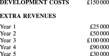
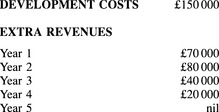
Figures 5.1.2 and 5.1.3 show simplified cash flows for the development of two new products – A and B. We shall use these simpler examples to compare the various techniques for a company which can only afford to invest £150000 at this point in time.
Payback period
This is the simplest and most commonly used technique. It basically calculates how long it takes to recover the initial investment. Taking the values in Figure 5.1.1, they come down to:
| Total outgoing | = | £109350 |
| Less sale of old machine | = | £3500 |
| Net investment | = | £105 850 |
| Savings | = | £33 500 |

This means that the investment will be paid back in three years and two months after the money starts to come in.
This method is often used as a hurdle with organizations, with management setting a minimum payback period – depending on the economic circumstances. In hard times, projects with more than a one year payback period could be rejected in many organizations.
Although this method is simple, it does suffer from several drawbacks:
Annual rate of return
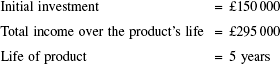
As can be seen in the payback examples, there can still be considerable benefits continuing after the payback period has been reached. To overcome the first of the drawbacks in the payback method, we have various methods. One way of comparing the total income over a project’s life against the investment is to calculate an annual rate of return. There are two ways to do this.
Average gross annual rate of return (AGARR)
The easiest way to demonstrate this is by working through the data for product A from Figure 5.1.2:

As can be seen the two products have different AGARR figures. Product A has a higher overall return, gives a higher AGARR, and is maintained for five years rather than the four years for product B.
It should be noted that product B has a higher initial recovery rate than product A. As we can surmise, high early returns are probably better than later returns, as later income can be reduced by unforeseen events, e.g. high inflation, new competition, drying up of supplies, etc. If we calculate a factor to take into account the time value of money, then the comparison between the investments may show up in different preferences. We will look at this after considering the other method of calculating annual rate of return:
As you can see the time period being considered makes a significant difference. The AGARR for product B now shows an even lower figure than that for product A as there is no income in the fifth year. The decision of what time to consider when comparing the two projects would depend on what happens at the end of product B’s life.
Average net annual rate of return (ANARR)
This method is similar to the AGARR method but with several key differences in calculating income and considering the investment. Again we will use the data for product A (from Figure 5.1.2) to show the process involved:

End value of investment = zero (no plant or equipment for resale)

The reason for taking an average for the investment is that the initial investment is being recovered, or paid back, by equal amounts each year. Therefore at the end of the product life the initial investment is fully paid back using this procedure.
Note that the ANARR is only slightly different than the AGARR value of 39.3% we calculated above in this example.
For product B, these ANARRs are significantly different from its AGARRs of 35% and 28% respectively. In this case, product A has a much better ANARR value of 38.7%. The ANARR method is a more severe method, especially when the net proceeds are small in relation to the initial investment.
However, both ANARR and AGARR ignore the time value of money.
Discounted cash flow (DCF) methods
When considering the value now of money earned or spent in the future, we can apply commonsense to see it will not be the same as the face value. What would you rather have − £1000 today, or £1000 next year?
How much extra would you wish to be paid one year from now in place of the £1000 today?
Obviously your answer would depend on a few factors such as how much you needed the £1000 today, how risky would it be to wait the year before payment, etc.
Businesses have the same problem – how much are future earnings worth today? The method they use to calculate the value of future earnings is called discounting. The discounting calculation is the inverse of the compounding calculation used for calculating the interest earned, or paid, on bank accounts, loans and mortgages.
Then discounting is the inverse of compounding:
Therefore if we wish to know what £1000 of next year’s money would be worth now if we discount at 10%, then:
Rather than have us calculate a discounting ratio each time, tables are produced to show a range of present values for different discount rates over a number of years. They are similar to that in Table 5.1.1 and are simple to use:

To find the present value of £1000 due in three years at a 10% discount rate, we look at the column headed 10% and move down it until we are on the three year row. We take that value – in this case 0.7513 – and multiply the future monetary value by it to find the present value:
We can see now how we discount future money to find present values. The only problem is ‘What do we select as the discount rate?’ The same hurdles are applied as with payback periods – high rates in hard times, easing when things look better.
To show the full process, let us again use the data for product A in Figure 5.1.2 with a discount factor or rate (DCF) of 20%. Where the flow is outward, i.e the initial investment, we use a negative value. Using a spreadsheet program such as Excel© to enter the data means it can easily be changed (see Figure 5.1.4).

Figure 5.1.4 shows a net present value (NPV) of £18 885.03, i.e. a positive value demonstrating that at a 20% discount rate the project would show a net profit of £18 885.03 at present values.
The calculation for product B shows a negative value which means it fails to show a profit in present value terms at the 20% discount rate. It would not proceed if 20% was the desired rate to be used for discounting.
Internal rate of return (IRR)
Using set rates of discount means that some projects can be rejected for failing to meet that criteria. It is probable that an organization could use different discount factors to take into consideration any risks involved. These discounted hurdle rates are often set arbitrarily.
There is, however, another method using discounting which can be employed. If we find the discount rate that would give exactly zero profit, we can compare different projects by using their equivalent discount rate. This rate where the discounted project returns zero is called the internal rate of return (IRR). The higher the IRR the better.
This rate can be found by a process of trial and error to find a rate that returns a net present value of zero.
A second way is to find an approximate value for the IRR by ratios. If we recalculate the net present value for product A (Figure 5.1.2) using a new discounted factor of 30%, we would arrive at a net present value of − £16 075.44. Therefore the IRR must lie between 20% and 30%.
If the relationship followed a straight line, then a graph showing the NPV between 20% and 30% DCF would cross the zero value in proportion to the differences:
Where ZV = point at which NPV = zero
Therefore IRR = 20% + 5.41 = 25.41%
The true line joining the NPV values is actually a concave curve – so the straight line taken is only approximate. By substituting the 25.41% into the CDF spreadsheet, we find a value of −£1519.76 showing that this approximate value is high.
The correct value is 24.97% found using the goal-seeking function in Excel© to discover the IRR (see Chapter 7 for this use of Excel©).
Both DCF and IRR are often a keystone in project appraisal.
Cash flow diagram
A good way to visualize the cash flow in a project is to draw a simple graph. Taking product A this would give a graph as shown in Figure 5.1.5.

Figure 5.1.5 Cash flow diagram for product A (Figure 5.1.2)
Looking at the graph it can be seen that the cash flow line crosses the x-axis at 2.75 years. This is the payback period or the breakeven point. The slope of the line shows how quickly the cash is flowing. Note, if you use the automatic Excel© graph function, it draws the line from the centre of each division and is therefore more difficult to read correctly.
Comparison between the appraisal techniques
As can be seen in Table 5.1.2, each technique gives a different judgement on the projects. Product B appears better in the payback period method, but product A gives better values for the remaining techniques, but not all to the same relative degree.

It is good practice to subject any appraisal figures to more than one process.
Integrating non-economic considerations into the selection process
Each of the projects can be compared under as many aspects as deemed desirable, perhaps by ranking them using the paired comparison technique (see Chapter 2 – page 93) to reduce them to the few main contenders.
The remaining contenders then need to be put through the organization’s economic appraisal system to determine their economic standing. There may be projects which require combining to determine their cross-effect on benefit and shared costs.
Once these stages have been completed, any remaining projects may need further ranking in priority. This can be carried out by producing a further matrix scoring each alternative on a scale from 1 (little impact) up to 10 (critical impact) under four or five significance criteria:
• Technical importance: Some projects must be completed before others can be advanced. This may be due to the lack of technical ability of the organization or a change in resources such as a new building or CAD systems.
• Financial investment: The full cost benefit analysis will show up the total amount of investment required. Here very high investment scores 1.
• Financial return: The time to pay back and total return can be judged here to determine future financial benefit.
• Competitive advantage: The impact on ability to deliver the order winning criteria demanded by our customer. These should tie in with the business plan.
• Intangible benefits: These could be factors such as staff turnover, public image, safety, environmental, etc. where the cash equivalent is difficult to determine. Scoring here could be on a perception basis.
All the criteria need not carry the same weighting. A survey of top management may decide at any one time that the criteria may be weighted as follows:

At another time they may increase the value of say, the financial investment to 2 because of cash flow problems.
From the scoring we can produce a priory grid as in Figure 5.1.6. The total in the second end column shows the total score against three projects under both weighted and non-weighted conditions. From these, the project with the highest weighted score would be selected for first priority – in this case alternative Y.

Time and other risks
It is important that a suitable time frame is selected to judge projects which do not have a clear life span.
If a short time frame is used then figures can be fairly accurately predicted. However, too short a frame can mean longer-term benefits could be missed. If too long a frame is used this increases the inaccuracy through uncertainty and risk due to unforeseen events, changing markets or changes in technology. Long term would also see plant deterioration, higher maintenance and even renewal.
There are other risks involved in any attempt to forecast markets (see Chapter 6, Section 6.2). These vary from changes in economic conditions, market behaviour, poor designs, competitors’ actions, war and natural disasters which may affect customers or suppliers.
Some allowance can be made for possible risks by scenario analysis (see Chapter 6, Section 6.4). It is also worthwhile to carry out a sensitivity analysis by varying some of the input information – such as plus or minus 10% on the sales figure, or the product life.
Non-financial factors
Although it is normally best to use monetary terms, these are sometimes difficult to determine, and resist attempts to express them in pure money terms. The benefits still need to be compared to the costs involved even if they cannot be quantified.
An example of this would be where new leading edge technology is being developed, but the actual improvements can be difficult to quantify initially. In Chapter 4, page 154, we examine one way of examining the overall effect of a project by considering the competitive advantage gained, the technical importance and other intangible benefits in addition to the financial value.
Perhaps the best question to ask in these circumstances is a simple one: ‘What happens if we do not make the investment?’
Problems 5.1.1
(1) Think about the last project you have been involved in. What were the benefits gained? Can you express all these benefits in money terms?
(2) Why do you think so many projects fail to make the returns envisaged in the case made for the investment?
(3) Why do you think that many companies request a payback period of less than one year for small capital projects?
(4) Do you think that all extra revenue spending, e.g. new product development, should be subjected to the same appraisal process as capital?
(5) Make out a case to justify spending your own money on a top-of-the-range personal computer for home use.
5.2 Cost determination
Management accounting is the name given to the allocation and control of internal costs within an organization. We need to understand how costs arise and vary to determine how to set them against products and services. For simplicity, we shall define services as being an intangible product.
As we mentioned in the previous section on investment appraisal, a business has one main aim – to earn more than it pays out over as short a time as possible. This applies especially to normal day-to-day running to accumulate profits which can then be used to fund investment and payback borrowings. No organization can survive unless it does make a profit. Even not-for-profit organizations such as charities cannot spend more than they receive in income, whatever the source.
The incoming revenue is based on the price we receive for products, or services. Profit is what is left after deducting all money spent.
Therefore to ensure that we do receive more money than we spend we have to ensure that prices more than cover all the costs involved. Prices themselves are difficult to control as they are often determined by what people will pay – not what a product costs. This leaves costs which are to be controlled. Unfortunately all the costs are not easy to set against particular products, or services.
Classifying costs
Costs can be described in two main ways.
Direct costs. This is a cost for any material or activity that is used directly in making the product. These costs include:
• Raw materials which go into the product.
• The labour operating machines, or assembling a product.
• Power and other consumables used up when making the product.
The easiest way to decide if a cost is direct is to ask the question – ‘If we make one more of this product, what actual money will need to be spent?’
There are other costs which are related to making a product such as machinery deterioration, maintenance, setting up the machine and inspection which we could perhaps try to classify as direct. This is often difficult and we shall return to how to set these against products later – for now, we shall treat these as indirect costs.
Indirect costs. These are all the costs which do not directly go into the making of the product. They include items such as supervision, general heating and lighting, administration, sales, etc. Note although these do not go directly into the making of a product, they are only there because the products are being made.
Behaviour of costs
Fixed costs. These do not vary as the amount of product made varies -at least in the short term as in Figure 5.2.1. In the long term they actually do vary – e.g. business rates change from year to year. Examples of these are rent and business rates, supervision, administration, etc. It should be obvious comparing this with indirect costs that fixed costs are in fact mainly indirect.

Variable costs. These should vary directly in relation to the products being made as in Figure 5.2.2. These can be seen as similar to direct costs.
Semi-variable costs. These are costs which do not vary in relation to slight variations in activity, but do in relation to significant changes. An example of this would be supervisors:
One supervisor may suffice to oversee 10 operatives, but if the number of operatives rose to 20, then an extra supervisor may have to be appointed. This behaviour is often stepped as in Figure 5.2.3.

What is slightly confusing is that many costs which are classified as variable can behave at times like a fixed cost, or behave in a less than directly proportional way. All supposedly fixed costs also vary – at least from year to year. We shall discuss this more later when looking at labour costs.
Costing
We shall now have a look at the way we set costs against products and services.
Labour
Labour costs are often thought of as easy. Just set the wages paid against product costs. In reality, it is more complex than that.
For example, it is difficult to employ part of an employee. We normally have to employ people for a set time period and may not have sufficient orders to keep them working for all the time we pay for. Their wage cost is then behaving as a fixed cost, or at least as a stepped cost.
Similarly an organization may have a human resource policy of not hiring and firing as trade fluctuates, making labour costs act very much like a fixed cost. Some organizations attempt to get round this by employing flexible part-time workers, but these are not always easy to find with the required skills.
Similarly the cost per hour of operatives can vary according to premiums for overtime, shift working and degree of skill. It is common within some industries to pay people a premium for having the capability of performing more than one skill e.g. being capable of operating more than one type of machine.
Labour cost elements
Labour costs must include more than just the basic pay that an employee receives. The extra costs involved are:
In addition, every minute of an employee’s time is not spent directly working on a product. There will be:
Everything done may not result in good products – some defective items will be produced involving either scrapping of work done, or reworking – which may be done by the same employee or a different one.
Finally there are overheads which are determined by the number of employees such as supervision, wages calculations, welfare and perhaps even recruitment if there is turnover of staff. However, let us leave these, to the discussion on overheads.
An example calculation is shown in Example 5.2.1.
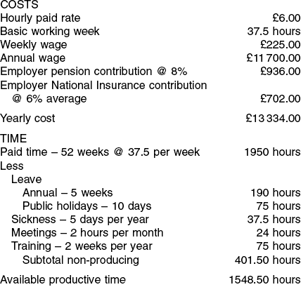
As we can see from Example 5.2.1, the actual cost rates per hour for employees are more than they are paid per hour. In this case, almost 44% more.
Note that this rate further assumes that all available time is actually spent on producing work. When allowing for non-productive time, cost per hour can readily approach double what an operative is paid for basic work time. If the employee in Example 5.2.1 was only 80% producing then the applied cost per hour would rise to £10.76–80% above his paid rate.
Controlling labour costs
From the above, it should be obvious that determining and controlling labour costs necessitates looking at a combination of factors:
• Premiums paid – for overtime, shifts, skills.
Being able to correctly identify the true cost rate means that product costs are accurate and decisions such as what product mix should be made or make-or-buy are based on reality.
Material costs
Similar to labour, at first sight determining material costs should be simple. Again, however, there are complications when we get down to details.
All material purchased does not leave the premises in the form of product:
• All processes have waste associated with them and this has to be included in any cost set against the product.
• There are losses due to scrap or reworking.
• Some materials are used in a process, but do not end up in the product – examples include emery powder (used for polishing), gas consumed in heat treatment and flux used in soldering.
In addition:
• Material which enters the premises causes other costs to arise such as receiving, handling, storage, stock-keeping, stock checking, deterioration, obsolescence, theft, etc.
• Money tied up in stock has a cost associated with it, e.g. interest.
• Even the purchase operation itself costs money to source the item, prepare an order, perhaps then to chase the order and, of course, eventually to pay the supplier.
Where possible therefore, we should determine all the associated costs and include them in the material cost when they happen.
Where material is ordered specifically for a job, then the cost of that material should be put against the job. This should happen even if there is material left over – that should only be excluded when it definitely will be used for another job or sold. In the latter instance the selling price of the material left over can be excluded. If reuse is only probable, then it cannot be excluded. If the material is thought not to be of use but is later sold, or used then it is a bonus.
An example of material bought for a particular job could be a 2 m by 1m sheet of 15 mm thick mild steel chequered plate (i.e. 2 m2). A rectangular piece measuring 1.23 m by 1 m is used (1.125 m2) leaving a piece measuring 0.25 m by 1 m. If there is no definite use for the off-cut then it must either be sold (and the price gained deducted from the initial material cost) or, if it cannot readily be sold, then the full amount of the material must be charged to the job.
In times when the prices of raw material fluctuate even determining the cost of standard stock material becomes more complex. This is because there are several methods of valuing stock material as it is withdrawn.
Even where materials are being used on a first-in-first-out basis, they can be valued in different ways. To demonstrate the differences, we shall look at the following material stock movements under four different valuation methods:
| 1 Jan | Zero stock |
| 2 Jan | Delivery: 1000 units @ £0.50 each |
| 9 Jan | Delivery: 1000 units @ £0.55 each |
| 11 Jan | Issue 800 units |
| 14 Jan | Issue 800 units |
| 16 Jan | Delivery: 1000 units @ £0.60 each |
| 18 Jan | Issue 800 units |
As the name implies, material usage is based on the earliest prices, until all material bought at that price is used up. It then moves onto the next price. The example is shown in Excel© format in Table 5.2.1.

As can be seen, the first received was 1000 units @ £0.50 each. These were the first to be issued for the 800 on 11 Jan – leaving 200 of the first receipt still in stock. When the next 800 were issued on 14 Jan only 200 units @ £0.50 each remained to be issued, the remaining 600 units had to be issued from the second receipt, i.e. @ £0.55 each.
Another receipt was on 16 Jan of 1000 units @ £0.60 each. For the issue on 18 Jan only 400 remained of that valued at £0.55. This left 400 to be issued at a value of £0.60. The stock remaining is all valued at £0.60 each.
This time value for the latest receipt is used for issues. The example is worked out in Table 5.2.2.

As can be seen, at the time of the first issue on 11 Jan, the last received were 1000 units @ £0.55 each. These were the first to be issued for the 800 on 11 Jan – leaving 200 of the next latest receipt still in stock. When the next 800 were issued on 14 Jan only 200 units @ £0.55 each remained to be issued, the remaining 600 units had to be issued from the first receipt, i.e. @ £0.50 each.
Another receipt was on 16 Jan of 1000 units @ £0.60 each. This value was used against the 800 issued on 18 Jan. The remaining stock consisted of 200 @ £0.60 and 400 @ £0.50.
In this method, the average price of the stock is recalculated after each receipt and this new average value is then used for any issues made before the next receipt (when average values need again be calculated). The example is shown in Table 5.2.3.

The two receipts on 2 and 9 Jan average out at a cost of £0.525. Note the Excel© sheet shown in Figure 5.2.3 has been set to show currency values to two places, but uses the true value to calculate values charged out.
This average figure is then used for issues until the receipt of 1000 units @ £0.60 each on 16 Jan when a recalculation of the average stock price has to be made. This new average price is then used for the material issued on 18 Jan.
In order to prevent recalculating an issue value each time an expected average, or standard, cost is often set at the beginning of a period for all issues. The example is shown in Table 5.2.4.

This time a standard issue cost of £0.55 was expected. Note that the actual cost of the material only agreed with the standard cost on one occasion. On the other two occasions, the actual price showed a variation from the standard set.
Comparison of methods
Table 5.2.5 shows the values of the issues out and of the remaining stock derived from the four methods. They are listed in order of issue value. No two have the same values. These differences will show up in the product cost calculation and the main profit and loss statement and the balance sheet.
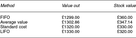
Any method can be decided on – as long as the organization always presents its information in the same way from one year to the next. It depends on whether the organization decides to make more emphasis on the items going as costs (value out) against profits or the valuation of its assets (stock value). In the long run, it does not matter too much as long as the method is clearly stated and consistently applied.
Controlling material costs
• Ensure all material, including waste and scrap is charged to the job.
• Determine true holding costs.
• Identify slow moving or obsolete stock.
The latter gives rise to systems such as material requirement planning (MRP) and just-in-time (JIT).
Process costs
We should build up a true picture of all the costs involved in operating an item of plant in a similar manner to that used to build up the cost of an operative-hour. First we have to determine what items of cost are caused by our operating that particular plant item. We then have to determine the monetary value to be set against the plant (see Example 5.2.2) for the budgeted number of running hours.
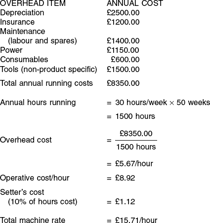
The overhead items of depreciation and insurance are independent of the running hours, but the remainder depend on the usage of the machine.
Note that the figure used for the operative rate was that calculated for the worker being available 100% of the time. However, only an 80% utilization has been used to calculate the overhead rate per hour. The remaining 20% could be set against a different cost area for control purposes. It should also be included in the machine hour rate, in which case this would rise to £18.93/hour.
Only 10% of a machine setter’s hourly cost rate has been set against the machine as that was calculated to be the amount of time the setter spent on the machine.
Where tooling is required specifically for a product then that cost should be set against the quantity to be produced by each tool.
Overheads
There are a multitude of activities which have to be carried out in a business which are difficult to directly attribute to a product, or process. These are the overheads in the business.
Allowing for ways to recover the cost of overheads is a major problem area in accounting. They must be covered for when deciding if a product is profitable or not at the price received.
If they are wrongly allowed for it could lead to incorrect decisions being made. Therefore it is always best to approach decision making on the same basis as investment appraisal, i.e. only consider overheads which will actually change when making decisions such as make-or-buy.
There are several ways to consider treating overheads.
Absorption costing
Under this method, we attempt to allocate all overheads to specific products, or processes. These overheads are then, in theory, recovered by producing products. This is sometimes referred to as full costing. The stages are:
(1) Select identifiable cost centres to collect and allocate costs from. This could be a particular group of machines or an indirect function such as maintenance.
(3) Allocate these overheads to cost centres where possible to identify their usage therein.
(4) Apportion unallocated costs using estimation of usage. This is often done arbitrarily.
(5) Apportion service departments into direct departments.
The absorption rates used vary considerably.
If a company had an overhead cost of £25 000 associated with a machine shop to be allocated it can choose from a variety of bases:
• Per unit produced: Cost centre overheads divided by number of units produced:
Example £25 000 over 100 000 units = £0.25 per unit
• Per labour hour: Cost centre overheads divided by direct labour hours.
Example £25 000 over 12 500 direct hours = £2.00 per hour
• Per machine hour: Cost centre overheads divided by direct machine hours.
Example £25 000 over 1000 machine hours = £25.00 per machine hour
• Per material usage: Cost centre overheads divided by direct material costs.
Example £25 000 over £50 000 material = £0.50 per £ material
• Floor space: Cost centre overheads divided by total floor area.
Only usage over time will dictate if the method selected is reasonable. Problems that arise are:
Marginal costing
Because of the problems of inaccuracy in overhead allocation, marginal costing is often used in decision making and determining the profitability of a product. In this method the variable costs, including accurately allocated overheads, are compared to the selling price. The difference is called the contribution.
The contribution has both to cover the unallocated overheads and add to the profit. This allows companies to gauge if there is a sufficient gap between selling price and variable costs.
As an example, if we sold 30 000 units of a product @ £3.50, which has £2.25 variable costs then:
If we have unallocated overheads of £25 000 then

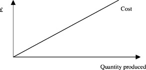
Marginal costing can be used to determine breakeven points. This is achieved by combining two costs (variable and overheads) into one graph and comparing it to the income against quantity produced as in Figure 5.2.4. Quite often this graph is used with fixed costs being used instead of overheads and as such it is similar to the cash flow diagram shown in Section 5.1.

However, as in absorption costing, marginal costing also has inherent complications:
Control of overhead costs
Overhead functions’ costs are not directly variable with units produced. They must still be controlled as they determine the profit left from the total contributions.
There are a few methods which are used to set initial budgets.
• Zero budgeting: This method is very similar to investment appraisal as in Section 5.1. Each overhead section has to justify its contribution towards profitability. In effect they have to prove that profits would be lower if they did not exist at certain levels.
• Activity based costing (ABC): It is recognized that different levels of activity result in cost level variations. ABC attempts to derive these causes, labelled cost drivers, so that the variations can be foreseen. An example of an activity would be salary and wage administration. Activity varies according to the number of people being paid and the wage systems employed.
The main activity after setting budgets is budgetary control.
Depreciation
When an organization purchases for use over several pieces of plant or equipment it does not put that cost in as a direct cost in the year of purchase. What it does is to assume that the plant’s value gets used up, or loses value, over a period of time. It therefore slowly feeds a part of that original cost into the direct cost over the plant life. This is termed depreciation.
Depreciation is a method used by accountants to transfer the loss in value of assets into an expense that is then transferred into the trading/profit and loss account. A similar approach can be taken to transfer development costs into the operating costs.
It is not like the other overhead costs as no actual money flows out of the company – that took place when the asset was purchased, or the development work took place.
There are several different methods for calculating depreciation within an organization, but only the two most commonly used methods are covered here – the straight line method and the reducing balance method.
The straight line method
This allows the same monetary value to be used each year.
For example, take an organization purchasing a new car for £20 000 and it plans to sell it in four years. It anticipates it will receive £10 000 for the car then:
If the same organization buys a new PC for £2400 that it estimates it will replace in 3 years with no resale potential then:
These examples are shown graphically in Figures 5.2.5 and 5.2.6 respectively.
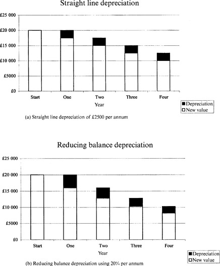

The reducing balance method
This allows a different value, i.e. a reducing amount, to be used each year.
If the same organization used the reducing balance method then if they decide that the car loses 20% per year, then they would have depreciation values as in Table 5.2.6.

In the case of the PC, if the company decides to use a 50% depreciation per annum factor then the depreciation in each year is as shown in Table 5.2.7.

As can be seen the closing values using the reducing value method are highly dependent on the factor used. In fact the residual value will never reach zero under this method. Graphs of these are also shown in Figures 5.2.5 and 5.2.6 which demonstrate the change in the depreciation from year to year.
The decision on which method to use is made by the organization itself. However, for tax purposes, a company is limited to the method, and values, laid down by government in what is termed capital allowances.
Typical UK government capital allowances are:
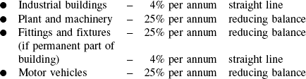
These are periodically subject to change and must be checked with the tax authorities each year. It is not uncommon for the values to be temporarily changed when a government wishes to encourage capital investment – for example, the UK government for the period 1999–2002 is allowing 100% capital allowances for IT investment, including developing E-commerce facilities.
Product costing
It is important when working out a product cost to agree beforehand the way overheads will be treated. This is very much down to company policy.
Probably it is best to use marginal costing with as many directly allocated overheads as possible in the calculation. Non-allocated overheads can be shown as a distinctly separate item if required.
The next is to ensure all costs are identified and how they will be applied to the costing. An important factor is the quantity to be produced as that will determine how items such as tooling, setting up and scrap allowance will be applied.
Detailed costings are required especially when considering different manufacturing processes.
If we take a one-off component as per Figure 5.2.7. There are many different ways to produce this. For this example let us assume it will be produced by machining from a 125 mm square bar.
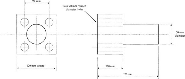
The first stage is to produce a process plan showing:
• What operations are required.
• What plant will be used to meet tolerance requirements.
• What time is involved for producing each one and for any set-up involved.
• Any special tooling required.
From these the costing can be done (see Table 5.2.8).
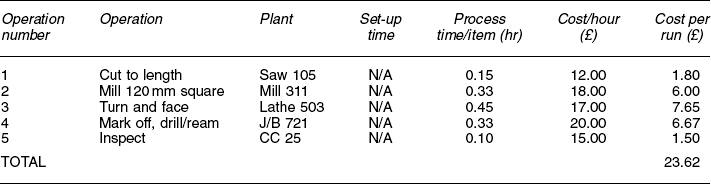
To this should be added the following costs:

As it is a one-off, then we should also consider extra costs such as raising the production order and the purchasing costs – say £30.
This means a direct cost of £23.62 + £9.50 + £3.50 + £30.00 = £66.62 to which should be added a mark-up percentage to contribute to non-allocated overheads and profits. This would probably mean a selling price of about £100 to cover all costs and give a reasonable profit.
It is worthwhile comparing what this cost would calculate as if we only used an average operator wage rate of £7.00 per hour. The total time involved is 1.03 hours. Multiplying by £7 gives £7.21. If we add material @ £9.50 a total of only £16.71 is arrived at. This is much less than the total arrived at when a detailed costing is carried out hence stressing the importance of carrying out a full costing.
Now what sort of change is involved when considering a large order quantity?
The first is that different processes would probably be selected and special tooling can be invested in.
This time we have a repeating order scheduled at 1000 off per month of the same component as per Figure 5.2.7. Let us assume this time it will be produced by machining from a special ordered 120 mm pre-finished square bar.
The first stage is again to produce a process plan from which the new costing can be done (see Table 5.2.9).

To this should be added the following costs:
• Raw material – bought in bars at £47.50 per metre. Required 250 mm finished length. Required length would be at least 250 mm plus an allowance for parting-off cutter and scrap at bar ends – say allow 280 mm per item. This gives a cost per item of £13.30, which is more than the one-off. This is because we have called for a special starting size, but it saves the operation of machining the 120 mm square.
• There is no allowance for inspection as this is considered to be an overhead in this case because 100% inspection is not necessary.
• Because it has moved operations (to higher producing machines which cost more per hour) we have to invest in special tooling. Special chuck jaws for the numerical controlled lathe and a drill jig for the multi-head drill machine. If these cost £2000 and £750 respectively there is a total tooling cost of £2750. We then have to decide how many units each tool will be written off against – in this case we shall use a year’s requirements of 12000 units. This gives a spread cost of £2750 divided by the 12000, i.e. 0.23 per unit.
• Delivery @ £0.50 each – because we have higher load usage, meaning lower cost.
• As it is a repeat order, we could also consider extra costs such as raising production order and purchasing costs as recoverable from the contribution. This means a direct cost of £2.90 + £13.30 + £0.50 + £0.23 = £16.93 to which should be added a slightly larger mark-up than in the case of the one-off mark-up percentage to contribute to the greater non-allocated overheads and profits. This would probably mean a selling price of around £30 to cover all costs and give a reasonable profit.
Problems 5.2.1
(1) What are the cost items which would be classified as direct costs when considering a car service at a garage?
(2) What is the cost rate per hour of overtime for the employee in Example 5.2.1, if a payment of 25% is made for overtime working? Hint: Only pension and National Insurance is added and there are no deductions for leave, etc. (£8.55)
(3) Compare the Automobile Association’s published figure of how much a small car costs per mile against a simple calculation of the cost of petrol used.
(4) How would you allow for recovery (payback) of the costs of developing a new product in the overhead costs?
(5) If you buy a new car, how much value does it lose in the first three years?
5.3 Producing the accounts
Financial accounting is the name given to the determination of the flow of money into, out of, and tracking what happens to this money inside, the organization. It measures the health of the organization.
There are three important documents which describe the financial health of the organization:
• The balance sheet – showing on one particular date where the money is within the organization and also what it is owed from and owed to the outside world. This is known as a snapshot of the financial position.
• The profit and loss account – showing over a set period the sales income, the cost to produce this, other operating expenses and the net profit. This shows the financial performance of the organization.
• Cash flow statement – showing the movement of money into and out of the organization.
Accounting standards
In order to ensure that potential suppliers and investors can examine all the company’s financial health in the same way, published accounts must conform to similar standards in presentation and content.
Legal requirements
The Companies Acts 1985 and 1989 prescribe that annually private companies must:
(a) Publish their profit and loss account.
(c) Adopt historical accounting rules (or permitted alternative).
(e) Publish Research and development activities.
(f) Publish a Source of increase or decrease in fixed assets, including revaluations.
Note: small and medium private companies need publish only limited information.
Accounts tend to follow recognized guidelines such as SSAP (Statement of Standard Accounting Practice) but this is not a legal requirement.
Concepts involved in financial accounting
• Money measurement: Only include items which are measured in monetary terms.
• Realization: When items are invoiced is normally the date used for determining when transactions have taken place. This means a cutoff date is selected to determine which account is credited/debited.
• Conservation or prudence – ‘Do not anticipate profits’ and ‘Provide for all possible losses’ are the guidelines. A good example is to allow for probable bad debts which will not be recovered.
• Matching: Accounts should show all money spent but only on activities carried out within the period.
– Accruals cover activities carried out, but not yet paid for, e.g. in arrears such as electricity.
– Prepayments are money paid in advance of future activity, e.g. rent.
• Consistency: Accounts must be calculated in same way from period to period.
• Disclosure: Any changes which have a significant effect on the accounts must be stated, e.g. a change in accounting practices.
• Objectivity: Endeavour to limit personal bias.
• Duality: The double entry principle. Every transaction is entered in two accounts – once as a debit and once as a credit.
• Verifiability: Accounts should be capable of being verified by independent auditors.
Cash flow statement
A very important day-to-day financial control that an organization carries out is over cash flow. More companies go out of business by running out of cash to pay their employees and suppliers than for being unprofitable.
Table 5.3.1 demonstrates a simple cash flow for a company in its second year of trading. Points to note are:
Table 5.3.1
Cash flow for year two of company. All values are shown in £s, unless otherwise stated. (Note figures in shaded background are paid in this year, but were incurred in the previous year and show up in the previous year’s profit and loss statement and balance sheet)
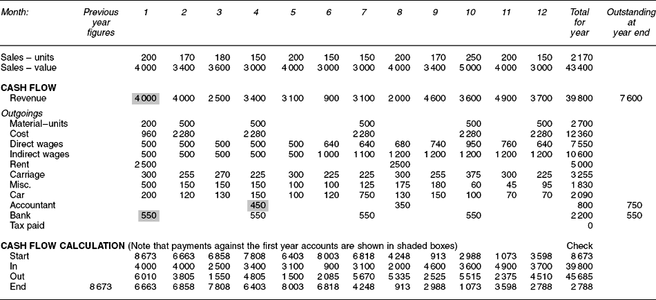
• All values are shown in £s, unless otherwise stated.
• Sales – shown in units (in italics) and value. Charged out at £20 each but paid for one month later (in arrears). The latter figure is shown in the Revenue row. This is when the cash is actually received and is the figure used when working out the cash flow.
• Materials – shown in units (in italics) and value. Purchased in quantities to make 500 units. Paid for @ £4.80 per unit on delivery.
• Premises are paid for six months in advance.
• Carriage is @ £1.50 per unit, paid in advance.
• The company borrowed £12 500 from the bank in the first year. Interest only is paid on this @ 16% per annum with bank charges of £50. Bank payments are made quarterly in arrears.
• Direct wages are paid to a part-time operator and include National Insurance.
• Indirect wages are the owner’s withdrawings as a salary and also include National Insurance.
• The following amounts are part of this year’s cash flow although they are items in the previous year’s profit and loss account and balance sheet (realization/matching concepts):
For simplicity, we are ignoring Value Added Tax (VAT), National Insurance Contribution (NIC) and pay-as-you-earn (PAYE) payments to government agencies. These were covered in Chapter 1 when dealing with external money transfers.
We can see from the cash flow figures that at all times a positive balance was maintained in cash.
Should this have become negative, then action would have to have been made. This could be arranging an overdraft or delaying some payment, but may be difficult to achieve in this example as most of the expenses had to be paid in advance due to little history of past successful trading by this organization. Companies with more history can normally arrange credit with their suppliers.
It is vital to make a budgeted cash flow for the future to determine when spending will occur and ensure that sufficient funds are available to cover it. Otherwise you would have to arrange an overdraft rather urgently.
The profit and loss account and the balance sheet
Using the data in Table 5.3.1, we will prepare these two interconnected accounting documents. The format we will use is called the vertical as all figures are complete in the one set of columns.
We require some further information on present material and product stocks, depreciation, and some information from last year’s balance sheet.
Stock and material usage
In this case we have no product stock. A similar calculation would have to be made if there was.
Note that the closing stock figure is entered into the balance sheet as a current asset.
Depreciation
This is calculated as shown in Figure 5.3.1 as part of the balance sheet and then transferred to the profit and loss account. In this case, the calculations have all been made on the basis of 25% of the old value. The new value of the asset is shown in the balance sheet.

Preparation of the profit and loss account
This proceeds using the above figures and the remaining information is transferred from the cash flow statement and shown in Figure 5.3.2. This gives two important values:

Figure 5.3.2 Preparation of balance sheet from cash flow statement. All values are shown in £s, unless otherwise stated
Note: no tax is due as no profit was made – the loss can be carried forward to set against any future profits.
We shall examine how well the company is doing by evaluating some key ratios in Section 5.4 later.
Completion of the balance sheet
This is completed by transferring data from the cash flow statement and the profit and loss accounts and is shown in Figure 5.3.1.
Net working capital shows the difference between short-term liabilities and short-term assets. The short-term liabilities include what is owed, but not paid. Net working capital should be positive to show that, in the short term, the business can repay its short-term liabilities through its short-term assets.
The reason for the balance sheet being so named is simple – it shows that the organization has a monetary balance between what it owns (the net short-term and long-term, or fixed, assets) and what it owes (the long-term liabilities, i.e. the capital employed made up of the owner’s investment and long-term loans). There should be no difference, i.e. they are in balance.
Any profit produced belongs to the owner – so any loss must also be borne by the owner, up to the limit of his liability. The reserve heading shown under owner investment denotes profit which has been retained in the business (i.e. not paid out as dividends, but still owed to the owners). It is produced by adding this year’s profit (or loss) retained to the previous year’s reserves.
In this case both the previous year’s and the current values have negative values. This means the net owner’s investment is decreasing –this is fairly common in a new company but requires careful monitoring so that a profitable stage is reached soon.
On the good side, there has been a positive cash flow over the last four months.
Some common items which have not occurred in this particular profit and loss account and balance sheet, but may in other companies, include:
• Allowance for bad debt. Some of the money owed may not be recovered because of customers going out of business, or fraud. This must come off the sales figure in the profit and loss account.
– Goodwill – an amount paid for another business over and above the physical value of the assets gained – this is depreciated just as a fixed asset.
– Intellectual property such as patents – sometimes difficult to value, but may be a source of earnings, or may be sold off to another business.
– Prepayment and accruals: If any made, or due to be paid then this should be entered. Prepayments would appear under current assets and accruals under current liabilities. Tax due could come under these headings, as could rent paid in advance.
– Revaluations: Where carried out, it must be described in accompanying notes with the basis of that revaluation.
Keeping the books
The process of book-keeping is one which often gives people problems in understanding. The basic process itself is simple – anyone who has a bank account should be able to understand entries. The difficulty comes in the multitude of different books and ledgers used, identifying which money flows where and making the many entries. Thankfully, modern accounting packages mean that the computer does most of the detailed entries.
Using the same data as in the cash flow shown in Table 5.3.1, the process is as follows.
The books
There are a multitude of separate accounts called books and ledgers (as that is what they once physically were). All transactions are recorded in them:
• Cash books: A book of first entry. Records cash and bank transactions.
• Day books: Also a book of first entry. Records cash and credit sales and purchases.
• Ledgers: Used to store and accumulate accounting information:
Meaningful classification of financial information is fundamental to its eventual usefulness. There are four basic types of accounts:
• Expenses and sales: These are normally used during the accounting period. They will be closed off and transferred to the trading, profit and loss account at the end of a trading period. They will restart in the next period with no entries.
• Assets and liabilities: These remain open at the end of a period as they normally have a residual value that will continue to be used by the organization in the future. They will be balanced and then their value will be copied to the balance sheet. This balance remains in these accounts to start off the next period.
The double entry system
Every financial transaction is listed in these accounts and involves an exchange of equal value shown as two associated entries – in different accounts. This is the double entry system.
• Whatever comes into the business is debited to an appropriate account.
• Whatever is going out of the business is credited to an appropriate account.
• Transferred amounts between accounts are shown as a debit entry and a corresponding credit entry.
You may think that accountants do the books in a mirror image to what you are used to seeing in your bank statements. This is because we are used to interpreting our bank balance from our viewpoint. The statement is correctly prepared looking at matters from the bank’s viewpoint. It is our definition of credit and debit that is different to those used in accounting. The problem is that our definition is becoming the norm outside accountancy – which causes problems when we first examine book-keeping.
Your deposit coming in is a debit on the bank’s cash book and this must have a corresponding credit entry in another account – yours. It is a liability on the bank to pay you. It sounds confusing; you may want to read these paragraphs again after we work through some examples.
It is important that you think of the terms debit and credit in the opposite way to that when you read your bank statement. This is the key to understanding book-keeping. Any money going in is a debit and money coming out is a credit.
Book and ledger accounts
If we take the data shown in the balance sheet (Figure 5.3.1), then we would have the following accounts. We will identify them, give them a code and classify them under the four headings.

The codes are to ease identification and reduce writing within the accounts when completing them. The terms used are historic and do not signify any real difference today. The codes used are:
CL = capital ledger – where long-term liabilities are recorded.
CA = capital asset – where long-term, i.e. fixed, assets are recorded.
CB = cash book – money in the bank.
PL = purchase ledger – purchases made.
SL = stock ledger – records of the value of stock (inventory).
There will also be other accounts such as tax due and dividend paid which are not activated yet. Later in the company’s life there could also be further accounts, or some accounts such as equipment could be split into transport, office and process plant.
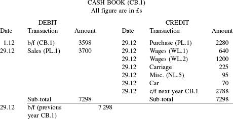
It will take some time to prepare full detailed accounts, so let’s start right at the beginning to show what happens with the initial money in the bank, i.e. the cash book. We shall assume that money flows take place on the last working day of the month:
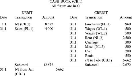
These entries should balance against each other at the end of January. The last entry on the credit side of £6662 is required to give this balance. Where there is a credit entry there must be an equal debit entry. That is made to reopen the cash book at the beginning of February. The terms c/f and b/f are abbreviations for carry forward and brought forward respectively.
All the credit entries above would have a corresponding entry in the noted account, for example:
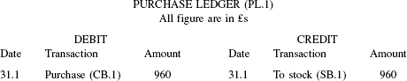
The value of the purchases are immediately transferred over to the stock account, which is a special account supplying information for both the balance sheet and the profit and loss account. It appears as a debit entry.
At the end of the accounting year, the b/f figure in the asset and liability accounts is copied into the balance sheet, but remains in the account as that b/f value:
This value opens the next year’s cash book account and is also copied (note – not transferred) to the balance sheet where it appears as a debit.
The stock account is actually an asset account and is the source for the stock figure copied to the balance sheet. However, it must contain a transaction to show the material usage.
If we look at this account, we find that up until the year end only the value of the opening stock and the purchases appear (in the debit column) to give a sub-total of £13 464. This is not the value that we have as physical stock as much of it has been used in manufacturing products.
At the year end, a physical stock check finds the actual closing stock to be £1710. The difference of £11 754 is attributed to the material used up in the manufacturing process.
Therefore on the credit side we show the closing stock value and an entry which is transferred to the profit and loss account, where it appears as a debit entry – remember double entry principle.
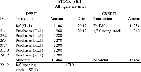
The opening/closing stock value is copied to the balance sheet.
This time we will use the credit/debit format to display the results. All asset accounts will appear on the debit side under long- or short-term headings. Liabilities appear as credit entries:
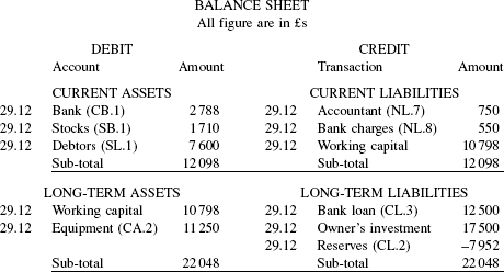
Both sides are in balance.
The working capital is the balancing value in the current assets and its double entry appears on the debit side in the long-term capital and liability section.
Similarly, we produce the profit and loss account by closing off all sales and expense accounts and transferring their balances to the profit and loss account, leaving them empty ready for the start of the new year’s trading.
Taking the direct wages account, we have:

Note: the sub-total for the debit entries has been transferred to the profit and loss account leaving a debit balance of zero to start off the next year.
The completed profit and loss account looks like:
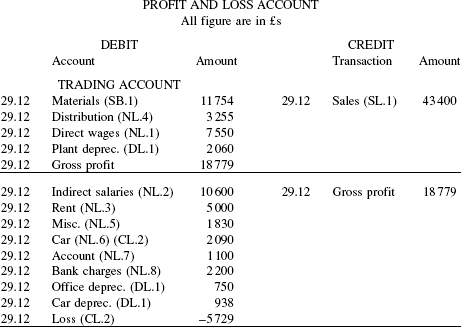
Again the totals balance.
The flow of the written transactions is shown in Figure 5.3.3.

In order to check during the financial year that all entries are being made correctly, many organizations carry out a trial balance (sheet) at other times than the year end. This is just a check process, it does not go into an end of year statement. Again with the increase in computer-based accounts this can be done speedily.
Problems 5.3.1
(1) What do you think will be a bank manager’s attitude if you suddenly had to seek an overdraft in the middle of your trading year?
(2) Can you think of other separate accounts that a company may wish to keep to add to the list on page 236?
(3) Try to complete the equipment account yourself. (Hint: use values already shown in Figure 5.3.1 for start values and depreciation.)
(4) Complete entries for another expense account – such as the indirect salary. (Hint: you can check your answer by looking at the balance sheet in Figure 5.3.1.)
(5) Get a public company’s published account and see if you can follow the cash flow over the year that produced the new balance sheet.
5.4 Budgeting and the interpretation of results
Once operations have been completed, it is possible to analyse how effective they have been in financial terms. This involves first developing a standard, or budget, breakdown of the expected costs and analysing why differences have occurred.
Everyone has personal experience of having to spend within a set budget. We have a finite income and many things we would like to buy, but we cannot buy all of them, as our money does not go far enough.
Every organization has the exact same problem as individuals do. Pressure to spend on items which will make life easier, more prestigious or more enjoyable, but a limited income. Every section has something they would like to spend money on – such as more people or a new computer.
We discussed in Section 5.1 techniques for justifying expenditure. These are difficult and time consuming to apply to every small decision that is made. We need another method that will enable managers, and increasingly other employees, to know how much they can spend and what they should be spending that money on. This is what budgeting is all about.
As when we produce a manpower plan (see Chapter 2, Section 2.1), we have to look at the future business plan for the organization. We then have to look at each department and section to see what resources are considered necessary to meet that plan. We cost these resources to produce a budgeted cash flow of the outgoing expenses and capital spending for each section (see Figure 5.4.1).

From these sections’ cash flows and the incoming money, we calculate what the overall resultant profit and loss will be. This is a long, and fairly tedious but necessary, task, which requires the involvement of all managers as this review sets what resources will be available during the budget period.
Only if the anticipated end result meets the business plan, can we say that we are relatively happy with the budget. Should the anticipated cash flow not meet the business plan then the budgets need to be revised until it does.
However, that is not the end of the story, we need to be continually comparing the actual cash flow with the budgeted cash flow to ensure that the targeted performance is met.
Preparing the budget
The best way to demonstrate this is to build a complete budget. We will take as our example the business that we showed the actual results for in Section 5.3. We will go back to the year before and build up a budget for the business.
Sales budget
The owner anticipated the annual sales would be 2400 @ £20 each. These he broke down into the following monthly figures:
Associated with these were materials, carriage and labour:
Labour was a little more problematic. The owner himself had been producing the units, but he was finding it difficult to find time to make them, sell them and spend time on developing a new product. He considered himself capable of making four units per hour. He planned to take on a part-time worker to train to manufacture the product. This would release the owner for selling and development.
This part-time operative was planned to be taken on in the fourth month. An initial allowance of £500 per month was made to cover 50 hours per month. This would start as a training budget and would reduce as the operative gradually came up to speed over a period of four months.
It was decided to make the standard labour cost of producing the sales figure £2.50 per unit. This was based on an expected cost of £10 per hour for the operative during which four units would be produced. The owner’s salary initially would be split using this figure with the remainder going into indirect wage cost. As the operative came up to speed, the portion set against the owner’s salary would reduce until by the eighth month it reduced to zero.
The owner then prepared a cash flow budget as in Table 5.4.1. The figures for miscellaneous and car expenses were estimated and spread over the year. The bank charges were considered to be the same as the first year and the accountant’s cost expected to be a little more.
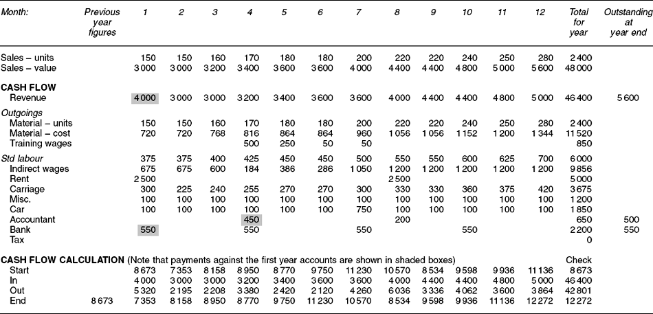
This produced a budgeted profit of £1399 (see Figure 5.4.2) which, although low, was reasonable as it was the business’s second year and the owner anticipated drawing £13 200 as a salary in addition. Although a profit was expected, no allowance was made for tax as the first year’s losses (£2223) could be offset against the anticipated year’s profits.

Analysing the results
Unfortunately, as we saw in Figure 5.3.2, the anticipated profits turned out to be a loss of £5729 − a difference of £7128 less than that budgeted for.
The anticipated figures are termed as the standard values. The differences we call variances and it is important that we analyse these variances and take action to rectify them, or make allowance for them if they are not changeable. To do this we should break the variance down into constituent causes:
There are different control formulae which can be used to analyse variances, i.e. the difference from that budgeted for:
These are the key ratios which we should keep our eye on to ensure that we are working efficiently and making effective use of our facilities on a time basis:
• Productivity performance: A measure of how effective our people are actually working. See appendix to Chapter 3 for further discussion on how to determine this. A suitable measure is:
• Capacity usage: This looks at how much of our people’s time we actually used in relation to what we set out to do in the budget. A suitable measure is:
• Volume index: Although this looks like the same as the productivity measure, it is using the hours that we originally set out to work as the base. It indicates how successful we were at bringing in work for them to do. A suitable measure is:
Note that these measures connect as follows:
• Sales revenue variance = (actual price/unit × actual sold) – (standard price/unit × budgeted sales)
• Selling price variance = (actual price – standard price)/unit × actual sold
• Sales effectiveness = (actual sold – budgeted sales) × standard price/unit
Note: Sales revenue variance = selling price variance + sales effectiveness.
These indicate the reason for having a revenue different to that anticipated. Was it the quantity sold, i.e. the sales effectiveness, or the price that was charged, i.e. the selling price variance.
• Material cost variance = (actual price/unit × actual usage) – (standard price/unit × standard for number produced)
• Purchase price variance = (actual price paid – standard price)/unit × actual usage
• Material usage variance = (actual usage – standard usage for number produced) × standard price/unit
Note: Material cost variance = purchase price variance + material usage variance.
These indicate the reason for having a material cost different to that anticipated. Was it the price paid for the material, i.e. the material price variance, or the amount of material used, i.e. the material usage variance?
• Labour cost variance = (actual hourly rate × actual hours) – (standard hourly rate × standard hours for units made)
• Labour rate variance = (actual hourly rate – standard hourly rate) × actual hours
• Labour efficiency = (actual hours – standard hours for number produced) × standard hourly rate
Note: Labour cost variance = labour rate variance + labour efficiency.
These indicate the reason for having a labour expense different to that anticipated. Was it how well we used the labour, i.e. the labour efficiency, or the hourly rate they were paid, i.e. the labour rate variance.
These formulae allow us to look beyond the straight variance and find underlying reasons. It enables us separate numerical and cost/price causes.
Let us go back to the example and compare the items in the actual profit and loss account against those budgeted for (see Figure 5.4.3).

When we see so many figures it can easily become a little confusing. What are the reasons for all these variations? For example, this analysis shows a favourable variance for distribution – is this good? Initially the answer may be yes, but as less was sold than budgeted for, we would expect a drop in spending on distribution.
To adjust those items which should vary with output, we can produce what is termed a flexed budget. This is simply adjusting the variable costs in line with sales by multiplying by the ratio of actual unit sales to the budgeted unit sales. We take units rather than monetary value, as we may have sold items at less than the standard price:
Most of the items going into the manufacturing costs can be taken as variable. If we apply the above calculation to them, we can then produce a variance analysis of flexed budget against actual costs as in Figure 5.4.4. The plant depreciation is left the same as budgeted for as this will not change.

Looking at this we can see that the distribution costs are in line with the actual sales. The revenue is also in line, hence price gained per item was as budgeted. However, materials and direct labour variances are even worse than they appeared before flexing. This needs further analysis, which will need more information than the cash flow statement and the profit and loss account figures show.
There were three reasons for the direct labour adverse variance of £1356 in the flexed budget comparison:
• The part-time operative was taken on in January rather than in April. However, the hourly cost for this was as expected – therefore no rate variance needs to be calculated.
• The training took longer than expected. This gave an adverse variance of £250.
• The expected output of four units per hour was not achieved -therefore we had an adverse efficiency variance of £1106 (based on the flexed budget figures). Probably the estimate of four units per hour made no allowance for break times, reworking and other lost time – it requires checking.
This may be slightly confusing as the unflexed direct labour variance is only an adverse one of £700. The difference in the figures is due to a favourable variance from the original budget of £656 due to lower actual sales. The latter only appears favourable because it is less than that original budgeted for.
When we look into the material costs, we find that two changes from the budget basis have taken place. More materials were used – but some were bought at a cheaper price. This calls for some examination of units used and prices paid per unit before we do the detailed variance calculations.
• Products produced were 2170.
• Budgeted material cost per unit was £4.80.
• After January’s purchases of 200 units, the owner started buying in bulk which gained him a discount of 5%, making the new cost of £4.56.
• Opening stock was £1104 valued at £4.80 each giving a unit stock of 230 (£1104 ÷ £4.80).
• Closing stock was £1710 valued at £4.56 each giving a unit stock of 375 (£1710 ÷ £4.56).
• Total units purchased was 2700 (200 at £4.80 and 2500 at £4.56).
Therefore we have a gain through buying cheaper (after the initial 200) but this has been offset by using more material. If we exclude the 200 bought at the budgeted cost, we can now see the monetary effect of these changes, using the following basis:
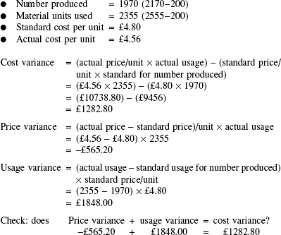


We can see that there was a favourable variance of £565.20 due to a lower purchasing price. This was not sufficient to offset the adverse variance of £1848.00 due to excess usage. Again this needs checking as it is about 20% extra usage which is a high figure. Perhaps some was consumed during early training which had not been allowed for.
Looking at the remaining expenses, the amount budgeted looks as if it may have been optimistic – but again this needs to be examined and explained.
Interpreting company accounts
In accountancy there are a number of ratios that are used to judge the effectiveness of an organization’s operations. These are worked out from the figures contained in the profit and loss account and the balance sheet.
The ratios normally require two consecutive years’ figures to work out an average over a company’s financial year. However, we shall use the one year’s result contained in Figures 5.3.2 and 5.3.2 for simplicity.
Return on investment
In any investment, there is an associated risk. Normally the possibility of a high return is linked to a high risk of getting considerably less – perhaps even losing the initial investment.
In the accounts the return is the net profit after all deductions for items such as depreciation and tax but before any dividend is paid. We need to divide this by the capital employed – however, there are several figures we can use as the divisor. Remember always check what figures are being used.
One way is to use the shareholder’s funds as the bottom line. Using the figures from our data, we have:

This means that the shareholders’ funds would be reduced to zero in just under three years if losses continued at this rate.
We could also use net assets, but we have to ensure that if a long-term loan is included in the funding then we add back onto the net profit any interest charges incurred by that loan.
The bank, however, will not let matters approach a point where their investment is too much at risk. They are liable to call in their loan before a further year has passed unless returns substantially increased.
Liquidity
If we examine the working capital of a company, we can see how quickly it can convert the current assets into cash to pay off the current liabilities. If we have a minus figure as working capital it demonstrates that we cannot meet our immediate needs and we are in trouble unless we can quickly find more cash.

Therefore,

Although both ratios are high, this is not necessarily a good indication. For example, if we could immediately convert our stocks and debtors into cash we could pay off 75% of our bank loan and save £1500 in interest charges.
We need to know the reason behind the figures and see if they can be changed to advantage:
• Being a new company, most of the purchasing is paid for in cash. We do not have credit with our supplier, as yet. If supplier credit could be obtained this would immediately reduce the need for cash, which could help to reduce the bank loan. Better to use our supplier’s money than our own.
• Customers should be paying for the goods after one month. The figure shown as owing indicates that they are taking longer and this puts pressure on cash flow. If they could be persuaded to pay early, even on delivery, again this would reduce the need for borrowing. Excess pressure to pay may lose us business and is a negative aspect we need to watch for.
• Raw material stocks represent almost two months’ supply –reducing these and only having enough to meet current needs would reduce this figure. It may be more costly buying more frequently, however.
Margins and mark-ups
In commercial terms margins can be expressed in two ways. It is important that we know exactly which figures are being used:
• Margins are based on the selling price – can look at gross and/or net figures.
• Mark-ups are based on costs (buying price or manufacturing) -again can look at gross or net figures.
Both are usually expressed as percentages.
Value added is another way of expressing mark-ups, and could be expressed as a monetary value.
In our examples, we have the following figures.

We could alternatively express the third of these items as gross profit = 76% mark-up on manufacturing costs. Similarly we could express the fourth item, Overheads, as being 99.5% of manufacturing costs.
Therefore to find the sales breakeven point, we need to apply the concept we used in Section 5.2 (page 222).
These figures are useful in letting us know by how much, if any, we can adjust prices when under customer pressure to do so to increase sales.
Turnover ratios
Turnover simply means the number of times in a period that an average item is used up and replaced. There are three important ratios relating to debtors, creditors and stock:
Debtor ratios. Only includes sales made on credit. In our example, no sales were for cash.
Therefore the customers are taking over twice as long to pay as the terms allow. Extra effort is required to shorten this time, but this may make our customers less eager to deal with us.
Creditor ratios. In our data, suppliers were paid on delivery. If, however, we assume that one month’s credit was allowed then:

This figure is a little misleading as the business does not purchase every month, but gives an idea of what levels can easily be attained to counteract debtors taking a long time to pay. Organizations should use creditors to balance the effect on cash flow of debtors.
Stock ratios. We can base this particular example on the cost of raw material only as no product stock is held. Where work-in-progress or product stock is held, we need to include it at the cost of manufacture – note not anticipated selling price.

As we mentioned when looking at the current ratio, this is high and should be reduced to release cash.
Gearing ratios
These indicate how the long-term funding of the company is supplied – loans or owners’ capital (shares and reserves). In the example at the end of year 2:

This indicates that currently the bank has a higher investment than the owner. This will make it difficult for the owner to ignore any suggestion made by the bank.
Share price ratios
The last set of ratios we are going to look at are related to share prices. Up until now we have not considered shares as our example has been based on a single owner.
In Chapter 1, we looked at the various patterns of ownership, and concluded that most of the large companies are funded by the issue of ordinary shares. These shares, once issued, are bought and sold in stock markets by their individual owners.
The shareholders are the owners of the company and as such can, and often do, have considerable influence on the management. The shareholders’ primal concern is not so much the present net value of the company assets but more the value of their shares. These two values can be considerably different.
Share prices can change considerably over a short period of time. The price is based on immediate factors and a mixture of other aspects regarding their future potential. We will not attempt here to value a business, just to describe how various ratios connected with shares are worked out.
To do this, we will need a new set of data, for a different organization. Again this has been simplified for ease of understanding:
• Issued shares: 5 million @ £1, equal to £5 million.
• Net profit after tax, but before payment of dividend: £1.2 million.
• Declared dividend for year: £0.12 per £1 share, giving a payout of £0.6 million.
The various concerns are:
Share price growth and stability
The P/E ratio of 9.37 represents the number of years to recoup the present share price based on present profits.
The actual share price will be affected by results from the organization and this must be taken into account when setting a strategy.
Problems 5.4.1
(1) Set down what your weekly income is and what your outgoings are. Are they the same? What can you do if your spending is more than your income?
(2) Compare the individual items in the actual profit and loss against that budgeted for in Figure 5.4.3. Why are some of the items up and some down. Is every figure bad?
(3) Is the drop in distribution costs in Figure 5.4.3 in line with the drop in sales from that budgeted for?
(4) Work out the percentage sales increase required to achieve breakeven, assuming no extra overhead spending is incurred. (31%)
(5) Get the published account of two public companies and see if you can explain the reason why the share prices are different.