
Chapter 4 Source Models
Most accidents in chemical plants result in spills of toxic, flammable, and explosive materials.
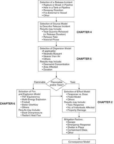
Source models are an important part of the consequence modeling procedure shown in Figure 4-1. More details are provided elsewhere.1 Accidents begin with an incident, which usually results in the loss of containment of material from the process. The material has hazardous properties, which might include toxic properties and energy content. Typical incidents might include the rupture or break of a pipeline, a hole in a tank or pipe, runaway reaction, or fire external to the vessel. Once the incident is known, source models are selected to describe how materials are discharged from the process. The source model provides a description of the rate of discharge, the total quantity discharged (or total time of discharge), and the state of the discharge (that is, solid, liquid, vapor, or a combination). A dispersion model is subsequently used to describe how the material is transported downwind and dispersed to some concentration levels. For flammable releases fire and explosion models convert the source model information on the release into energy hazard potentials, such as thermal radiation and explosion over-pressures. Effect models convert these incident-specific results into effects on people (injury or death) and structures. Environmental impacts could also be considered, but we do not do so here. Additional refinement is provided by mitigation factors, such as water sprays, foam systems, and sheltering or evacuation, which tend to reduce the magnitude of potential effects in real incidents.
1Guidelines for Consequence Analysis of Chemical Releases (New York: American Institute of Chemical Engineers, 1999).
Figure 4-1 Consequence analysis procedure. Adapted from Guidelines for Consequence Analysis for Chemical Releases (New York: American Institute of Chemical Engineers, 1999).
4-1 Introduction to Source Models
Source models are constructed from fundamental or empirical equations representing the physicochemical processes occurring during the release of materials. For a reasonably complex plant many source models are needed to describe the release. Some development and modification of the original models is normally required to fit the specific situation. Frequently the results are only estimates because the physical properties of the materials are not adequately characterized or because the physical processes themselves are not completely understood. If uncertainty exists, the parameters should be selected to maximize the release rate and quantity. This ensures that a design is on the safe side.
Release mechanisms are classified into wide and limited aperture releases. In the wide aperture case a large hole develops in the process unit, releasing a substantial amount of material in a short time. An excellent example is the overpressuring and explosion of a storage tank. For the limited aperture case material is released at a slow enough rate that upstream conditions are not immediately affected; the assumption of constant upstream pressure is frequently valid.
Limited aperture releases are conceptualized in Figure 4-2. For these releases material is ejected from holes and cracks in tanks and pipes, leaks in flanges, valves, and pumps, and severed or ruptured pipes. Relief systems, designed to prevent the overpressuring of tanks and process vessels, are also potential sources of released material.
Figure 4-2 Various types of limited aperture releases.
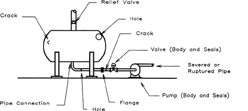
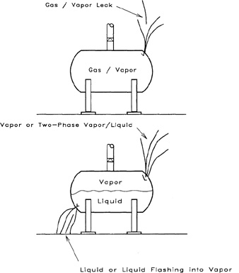
Figure 4-3 shows how the physical state of the material affects the release mechanism. For gases or vapors stored in a tank, a leak results in a jet of gas or vapor. For liquids a leak below the liquid level in the tank results in a stream of escaping liquid. If the liquid is stored under pressure above its atmospheric boiling point, a leak below the liquid level will result in a stream of liquid flashing partially into vapor. Small liquid droplets or aerosols might also form from the flashing stream, with the possibility of transport away from the leak by wind currents. A leak in the vapor space above the liquid can result in either a vapor stream or a two-phase stream composed of vapor and liquid, depending on the physical properties of the material.
Figure 4-3 Vapor and liquid are ejected from process units in either single- or two-phase states.
There are several basic source models that are used repeatedly and will be developed in detail here. These source models are
• flow of liquid through a hole,
• flow of liquid through a hole in a tank,
• flow of liquids through pipes,
• flow of vapor through holes,
• flow of gases through pipes,
• flashing liquids, and
• liquid pool evaporation or boiling.
Other source models, specific to certain materials, are introduced in subsequent chapters.
4-2 Flow of Liquid through a Hole
A mechanical energy balance describes the various energy forms associated with flowing fluids:
(4-1)
![]()
where
P is the pressure (force/area),
ρ is the fluid density (mass/volume),
ū is the average instantaneous velocity of the fluid (length/time),
gc is the gravitational constant (length mass/force time2),
α is the unitless velocity profile correction factor with the following values:
α = 0.5 for laminar flow, α = 1.0 for plug flow, and α → 1.0 for turbulent flow,
g is the acceleration due to gravity (length/time2),
z is the height above datum (length),
F is the net frictional loss term (length force/mass),
Ws is the shaft work (force length), and
m is the mass flow rate (mass/time).
The Δ function represents the final minus the initial state.
For incompressible liquids the density is constant, and
(4-2)
![]()
Consider a process unit that develops a small hole, as shown in Figure 4-4. The pressure of the liquid contained within the process unit is converted to kinetic energy as the fluid escapes through the leak. Frictional forces between the moving liquid and the wall of the leak convert some of the kinetic energy of the liquid into thermal energy, resulting in a reduced velocity.
Figure 4-4 Liquid escaping through a hole in a process unit. The energy of the liquid resulting from its pressure in the vessel is converted to kinetic energy, with some frictional flow losses in the hole.
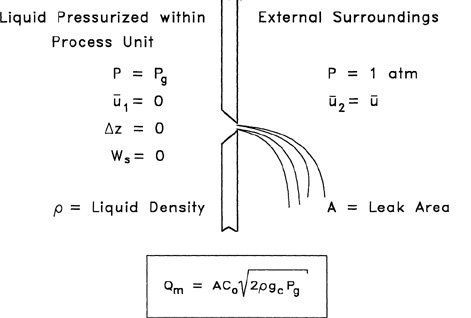
For this limited aperture release, assume a constant gauge pressure Pg, within the process unit. The external pressure is atmospheric; so ΔP = Pg. The shaft work is zero, and the velocity of the fluid within the process unit is assumed negligible. The change in elevation of the fluid during the discharge through the hole is also negligible; so Δz = 0. The frictional losses in the leak are approximated by a constant discharge coefficient Cl, defined as
(4-3)
![]()
The modifications are substituted into the mechanical energy balance (Equation 4-1) to determine ū, the average discharge velocity from the leak:
(4-4)
![]()
A new discharge coefficient Co, is defined as
(4-5)
![]()
The resulting equation for the velocity of fluid exiting the leak is
(4-6)
![]()
The mass flow rate Qm resulting from a hole of area A is given by
(4-7)
![]()
The total mass of liquid spilled depends on the total time that the leak is active.
The discharge coefficient Co is a complicated function of the Reynolds number of the fluid escaping through the leak and the diameter of the hole. The following guidelines are suggested:2
2Frank P. Lees, Loss Prevention in the Process Industries, 2d ed. (London: Butterworths, 1996); p. 15/7.
• For sharp-edged orifices and for Reynolds numbers greater than 30,000, Co approaches the value 0.61. For these conditions the exit velocity of the fluid is independent of the size of the hole.
• For a well-rounded nozzle the discharge coefficient approaches 1.
• For short sections of pipe attached to a vessel (with a length-diameter ratio not less than 3), the discharge coefficient is approximately 0.81.
• When the discharge coefficient is unknown or uncertain, use a value of 1.0 to maximize the computed flows.
More details on discharge coefficients for these types of liquid discharges are provided elsewhere.3
3Robert H. Perry and Don W. Green, Perry’s Chemical Engineers Handbook, 7th ed. (New York: McGraw-Hill, 1997), pp. 10–16.
Example 4-1
At 1 P.M. the plant operator notices a drop in pressure in a pipeline transporting benzene. The pressure is immediately restored to 100 psig. At 2:30 P.M. a 1/4-in-diameter leak is found in the pipeline and immediately repaired. Estimate the total amount of benzene spilled. The specific gravity of benzene is 0.8794.
Solution
The drop in pressure observed at 1 P.M. is indicative of a leak in the pipeline. The leak is assumed to be active between 1 P.M. and 2:30 P.M., a total of 90 minutes. The area of the hole is
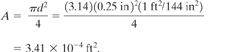
The density of the benzene is
![]()
The leak mass flow rate is given by Equation 4-7. A discharge coefficient of 0.61 is assumed for this orifice-type leak:
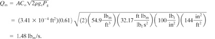
The total quantity of benzene spilled is
(1.48 lbm/s)(90 min)(60 s/min) = 7990 lbm 1090gal.
4-3 Flow of Liquid through a Hole in a Tank
A storage tank is shown in Figure 4-5. A hole develops at a height hL below the fluid level. The flow of liquid through this hole is represented by the mechanical energy balance (Equation 4-1) and the incompressible assumption, as shown in Equation 4-2.
Figure 4-5 An orifice-type leak in a process vessel. The energy resulting from the pressure of the fluid height above the leak is converted to kinetic energy as the fluid exits through the hole. Some energy is lost because of frictional fluid flow.
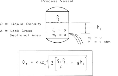
The gauge pressure on the tank is Pg, and the external gauge pressure is atmospheric, or 0. The shaft work Ws is zero, and the velocity of the fluid in the tank is zero.
A dimensionless discharge coefficient Cl, is defined as
(4-8)
![]()
The mechanical energy balance (Equation 4-1) is solved for the average instantaneous discharge velocity from the leak:
(4-9)
![]()
where hL is the liquid height above the leak. A new discharge coefficient Co is defined as
(4-10)
![]()
The resulting equation for the instantaneous velocity of fluid exiting the leak is
(4-11)
![]()
The instantaneous mass flow rate Qm resulting from a hole of area A is given by
(4-12)
![]()
As the tank empties, the liquid height decreases and the velocity and mass flow rate decrease.
Assume that the gauge pressure Pg on the surface of the liquid is constant. This would occur if the vessel was padded with an inert gas to prevent explosion or was vented to the atmosphere. For a tank of constant cross-sectional area At, the total mass of liquid in the tank above the leak is
(4-13)
![]()
The rate of change of mass within the tank is
(4-14)
![]()
where Qm is given by Equation 4-12. By substituting Equations 4-12 and 4-12 into Equation 4-14 and by assuming constant tank cross-section and liquid density, we can obtain a differential equation representing the change in the fluid height:
(4-15)
![]()
Equation 4-15 is rearranged and integrated from an initial height hLo to any height hL:
(4-16)
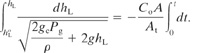
This equation is integrated to
(4-17)
![]()
Solving for hL, the liquid level height in the tank, yields
(4-18)
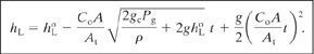
Equation 4-18 is substituted into Equation 4-12 to obtain the mass discharge rate at any time t :
(4-19)
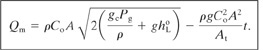
The first term on the right-hand side of Equation 4-19 is the initial mass discharge rate at hL = hoL
The time te for the vessel to empty to the level of the leak is found by solving Equation 4-18 for t after setting hL = 0:
(4-20)
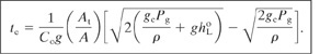
If the vessel is at atmospheric pressure, Pg 0 and Equation 4-20 reduces to
(4-21)
![]()
Example 4-2
A cylindrical tank 20 ft high and 8 ft in diameter is used to store benzene. The tank is padded with nitrogen to a constant regulated pressure of 1 atm gauge to prevent explosion. The liquid level within the tank is presently at 17 ft. A 1-in puncture occurs in the tank 5 ft off the ground because of the careless driving of a forklift truck. Estimate (a) the gallons of benzene spilled, (b) the time required for the benzene to leak out, and (c) the maximum mass flow rate of benzene through the leak. The specific gravity of benzene at these conditions is 0.8794.
Solution
The density of the benzene is
![]()
The area of the tank is
![]()
The area of the leak is
![]()
The gauge pressure is
![]()
a. The volume of benzene above the leak is
![]()
This is the total benzene that will leak out.
b. The length of time for the benzene to leak out is given by Equation 4-20:
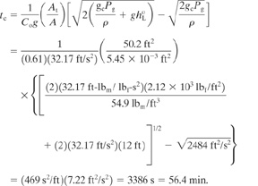
This appears to be more than adequate time to stop the leak or to invoke an emergency procedure to reduce the impact of the leak. However, the maximum discharge occurs when the hole is first opened.
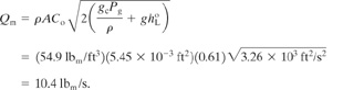
c. The maximum discharge occurs at t = 0 at a liquid level of 17.0 ft. Equation 4-19 is used to compute the mass flow rate:
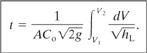
A general equation to represent the draining time for any vessel of any geometry is developed as follows. Assume that the head space above the liquid is at atmospheric pressure; then combining Equations 4-12 and 4-12, we get
(4-22)
![]()
By rearranging and integrating, we obtain
(4-23)
![]()
which results in the general equation for the draining time for any vessel:
(4-24)
Equation 4-24 does not assume that the hole is at the bottom of the vessel.
For a vessel with the shape of a vertical cylinder, we have
(4-25)
![]()
By substituting into Equation 4-24, we obtain
(4-26)
![]()
If the hole is at the bottom of the vessel, then Equation 4-26 is integrated from h = 0 to h = ho. Equation 4-26 then provides the emptying time for the vessel:
(4-27)
![]()
which is the same result as Equation 4-21.
4-4 Flow of Liquids through Pipes
A pipe transporting liquid is shown in Figure 4-6. A pressure gradient across the pipe is the driving force for the movement of liquid. Frictional forces between the liquid and the wall of the pipe convert kinetic energy into thermal energy. This results in a decrease in the liquid velocity and a decrease in the liquid pressure.
Figure 4-6 Liquid flowing through a pipe. The frictional flow losses between the fluid and the pipe wall result in a pressure drop across the pipe length. Kinetic energy changes are frequently negligible.
Flow of incompressible liquids through pipes is described by the mechanical energy balance (Equation 4-1) combined with the incompressible fluid assumption (Equation 4-2). The net result is
(4-28)
![]()
The frictional loss term F in Equation 4-28 represents the loss of mechanical energy resulting from friction and includes losses resulting from flow through lengths of pipe; fittings such as valves, elbows, orifices; and pipe entrances and exits. For each frictional device a loss term of the following form is used:
(4-29)
![]()
where
Kf is the excess head loss due to the pipe or pipe fitting (dimensionless) and
u is the fluid velocity (length/time).
For fluids flowing through pipes the excess head loss term Kf is given by
(4-30)
![]()
where
f is the Fanning friction factor (unitless),
L is the flow path length (length), and
d is the flow path diameter (length).
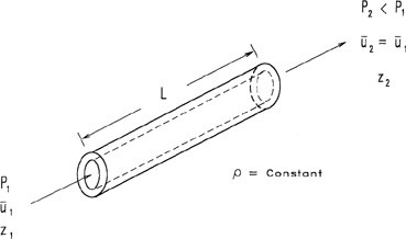
The Fanning friction factor f is a function of the Reynolds number Re and the roughness of the pipe ε. Table 4-1 provides values of ε for various types of clean pipe. Figure 4-7 is a plot of the Fanning friction factor versus Reynolds number with the pipe roughness, ε/d, as a parameter.
Table 4-1 Roughness Factor ε for Clean Pipes1
1Selected from Octave Levenspiel, Engineering Flow and Heat Exchange (New York: Plenum Press, 1984), p. 22.
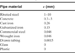
Figure 4-7 Plot of Fanning friction factor f versus Reynolds number. Source: Octave Levenspiel, Engineering Flow and Heat Exchange (New York: Plenum Press, 1984), p. 20. Reprinted by permission.
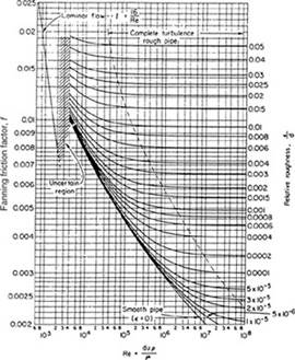
For laminar flow the Fanning friction factor is given by
(4-31)
![]()
For turbulent flow the data shown in Figure 4-7 are represented by the Colebrook equation:
(4-32)
![]()
An alternative form of Equation 4-32, useful for determining the Reynolds number from the friction factor f, is
(4-33)
![]()
For fully developed turbulent flow in rough pipes, f is independent of the Reynolds number, as shown by the nearly constant friction factors at high Reynolds number in Figure 4-7. For this case Equation 4-33 is simplified to
(4-34)
![]()
For smooth pipes, ε = 0 and Equation 4-32 reduces to
(4-35)
![]()
For smooth pipe with a Reynolds number less than 100,000 the following Blasius approximation to Equation 4-35 is useful:
(4-36)
![]()
A single equation has been proposed by Chen4 to provide the friction factor f over the entire range of Reynolds numbers shown in Figure 4-7. This equation is
4N. H. Chen, Industrial Engineering and Chemistry Fundamentals (1979), 18: 296.
(4-37)
![]()
where
![]()
2-K Method
For pipe fittings, valves, and other flow obstructions the traditional method has been to use an equivalent pipe length Lequiv in Equation 4-30. The problem with this method is that the specified length is coupled to the friction factor. An improved approach is to use the 2-K method,5,6 which uses the actual flow path length in Equation 4-30 — equivalent lengths are not used — and provides a more detailed approach for pipe fittings, inlets, and outlets. The 2-K method defines the excess head loss in terms of two constants, the Reynolds number and the pipe internal diameter:
5W. B. Hooper, Chemical Engineering, (Aug. 24, 1981), pp. 96–100.
6W. B. Hooper, Chemical Engineering, (Nov. 7, 1988), pp. 89–92.
(4-38)
![]()
where
Kf is the excess head loss (dimensionless),
Kl and K∞ are constants (dimensionless),
Re is the Reynolds number (dimensionless), and
IDinches is the internal diameter of the flow path (inches).
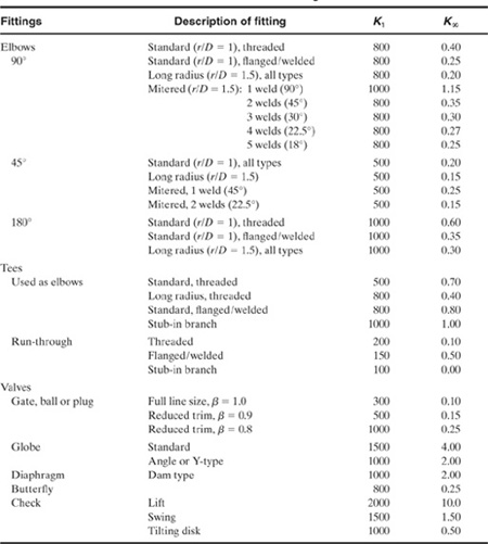
Table 4-2 contains a list of K values for use in Equation 4-38 for various types of fittings and valves.
Table 4-2 2-K Constants for Loss Coefficients in Fittings and Valves1
1William B. Hooper, Chemical Engineering, (Aug. 24, 1981), p. 97.
For pipe entrances and exits Equation 4-38 is modified to account for the change in kinetic energy:
(4-39)
![]()
For pipe entrances, K1 = 160 and K∞ = 0.50 for a normal entrance and K∞ = 1.0 for a Borda-type entrance. For pipe exits, K1 = 0 and K∞ = 1.0. The K factors for the entrance and exit effects account for the changes in kinetic energy through these piping changes, so no additional kinetic energy terms in the mechanical energy balance must be considered. For high Reynolds numbers (that is, Re > 10,000) the first term in Equation 4-39 is negligible and Kf = K∞. For low Reynolds numbers (that is, Re < 50) the first term dominates and Kf = K1/Re.
Equations are also available for orifices7 and for changes in pipe sizes.8
7W. B. Hooper, Chemical Engineering, (Aug. 24, 1981), pp. 96–100.
8W. B. Hooper, Chemical Engineering, (Nov. 7, 1988), pp. 89–92.
The 2-K method also represents liquid discharge through holes. From the 2-K method an expression for the discharge coefficient for liquid discharge through a hole can be determined. The result is
(4-40)
![]()
where ∑ Kf is the sum of all excess head loss terms, including entrances, exits, pipe lengths, and fittings, provided by Equations 4-30, 4-38, and 4-39. For a simple hole in a tank with no pipe connections or fittings the friction is caused only by the entrance and exit effects of the hole. For Reynolds numbers greater than 10,000, Kf = 0.5 for the entrance and Kf = 1.0 for the exit. Thus ∑ Kf = 1.5, and from Equation 4-40, Co = 0.63, which nearly matches the suggested value of 0.61.
The solution procedure to determine the mass flow rate of discharged material from a piping system is as follows:
1. Given: the length, diameter, and type of pipe; pressures and elevation changes across the piping system; work input or output to the fluid resulting from pumps, turbines, etc.; number and type of fittings in the pipe; properties of the fluid, including density and viscosity.
2. Specify the initial point (point 1) and the final point (point 2). This must be done carefully because the individual terms in Equation 4-28 are highly dependent on this specification.
3. Determine the pressures and elevations at points 1 and 2. Determine the initial fluid velocity at point 1.
4. Guess a value for the velocity at point 2. If fully developed turbulent flow is expected, then this is not required.
5. Determine the friction factor for the pipe using Equations 4-31 through 4-37.
6. Determine the excess head loss terms for the pipe (using Equation 4-30), for the fittings (using Equation 4-38), and for any entrance and exit effects (using Equation 4-39). Sum the head loss terms, and compute the net frictional loss term using Equation 4-29. Use the velocity at point 2.
7. Compute values for all the terms in Equation 4-28, and substitute into the equation. If the sum of all the terms in Equation 4-28 is zero, then the computation is completed. If not, go back to step 4 and repeat the calculation.
8. Determine the mass flow rate using the equation ![]()
If fully developed turbulent flow is expected, the solution is direct. Substitute the known terms into Equation 4-28, leaving the velocity at point 2 as a variable. Solve for the velocity directly.
Example 4-3
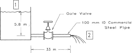
Water contaminated with small amounts of hazardous waste is gravity-drained out of a large storage tank through a straight commercial steel pipe, 100 mm ID (internal diameter). The pipe is 100 m long with a gate valve near the tank. The entire pipe assembly is mostly horizontal. If the liquid level in the tank is 5.8 m above the pipe outlet, and the pipe is accidently severed 33 m from the tank, compute the flow rate of material escaping from the pipe.
Solution
The draining operation is shown in Figure 4-8. Assuming negligible kinetic energy changes, no pressure changes, and no shaft work, the mechanical energy balance (Equation 4-28) applied between points 1 and 2 reduces to
![]()
Figure 4-8 Draining geometry for example 4-3.
For water
μ = 1.0 10-3 kg/m s,
p = 1000 kg/m3.
The K factors for the entrance and exit effects are determined using Equation 4-39. The K factor for the gate valve is found in Table 4-2, and the K factor for the pipe length is given by Equation 4-30. For the pipe entrance,
![]()
For the gate valve,
![]()
For the pipe exit,
Kf = 1.0
For the pipe length,
![]()
Summing the K factors gives
![]()
For Re > 10,000 the first term in the equation is small. Thus
![]()
and it follows that
![]()
The gravitational term in the mechanical energy equation is given by
![]()
Because there is no pressure change and no pump or shaft work, the mechanical energy balance (Equation 2-28) reduces to
![]()
Solving for the exit velocity and substituting for the height change gives
![]()
The Reynolds number is given by
![]()
For commercial steel pipe, from Table 4-1, ε = 0.0046 mm and
![]()
Because the friction factor f and the frictional loss term F are functions of the Reynolds number and velocity, the solution is found by trial and error. The trial and error solution is shown in the following table:
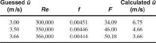
Thus the velocity of the liquid discharging from the pipe is 3.66 m/s. The table also shows that the friction factor f changes little with the Reynolds number. Thus we can approximate it using Equation 4-34 for fully developed turbulent flow in rough pipes. Equation 4-34 produces a friction factor value of 0.0041. Then
![]()
By substituting and solving, we obtain
This result is close to the more exact trial and error solution.
The cross-sectional area of the pipe is
![]()
The mass flow rate is given by
Qm = ρ![]() A = (1000 kg/m3)(3.66 m/s)(0.00785 m2) = 28.8kg/s
A = (1000 kg/m3)(3.66 m/s)(0.00785 m2) = 28.8kg/s
This represents a significant flow rate. Assuming a 15-min emergency response period to stop the release, a total of 26,000 kg of hazardous waste will be spilled. In addition to the material released by the flow, the liquid contained within the pipe between the valve and the rupture will also spill. An alternative system must be designed to limit the release. This could include a reduction in the emergency response period, replacement of the pipe by one with a smaller diameter, or modification of the piping system to include additional control valves to stop the flow.
4-5 Flow of Vapor through Holes
For flowing liquids the kinetic energy changes are frequently negligible and the physical properties (particularly the density) are constant. For flowing gases and vapors these assumptions are valid only for small pressure changes (P1/P2 < 2) and low velocities (< 0.3 times the speed of sound in gas). Energy contained within the gas or vapor as a result of its pressure is converted into kinetic energy as the gas or vapor escapes and expands through the hole. The density, pressure, and temperature change as the gas or vapor exits through the leak.
Gas and vapor discharges are classified into throttling and free expansion releases. For throttling releases the gas issues through a small crack with large frictional losses; little of the energy inherent to the gas pressure is converted to kinetic energy. For free expansion releases most of the pressure energy is converted to kinetic energy; the assumption of isentropic behavior is usually valid.
Source models for throttling releases require detailed information on the physical structure of the leak; they are not considered here. Free expansion release source models require only the diameter of the leak.
A free expansion leak is shown in Figure 4-9. The mechanical energy balance (Equation 4-1) describes the flow of compressible gases and vapors. Assuming negligible potential energy changes and no shaft work results in a reduced form of the mechanical energy balance describing compressible flow through holes:
Figure 4-9 A free expansion gas leak. The gas expands isentropically through the hole. The gas properties (ρ, T) and velocity change during the expansion.
(4-41)
![]()
A discharge coefficient Cl, is defined in a similiar fashion to the coefficient defined in section 4-2:
(4-42)
![]()
Equation 4-42 is combined with Equation 4-41 and integrated between any two convenient points. An initial point (denoted by subscript “o”) is selected where the velocity is zero and the pressure is Po. The integration is carried to any arbitrary final point (denoted without a subscript). The result is
(4-43)
![]()
For any ideal gas undergoing an isentropic expansion,
(4-44)
![]()
where γ is the ratio of the heat capacities, γ = Cρ/Cv. Substituting Equation 4-44 into Equation 4-43, defining a new discharge coefficient Co identical to that in Equation 4-5, and integrating results in an equation representing the velocity of the fluid at any point during the isentropic expansion:
(4-45)
![]()
The second form incorporates the ideal gas law for the initial density ρo. Rg is the ideal gas constant, and To is the temperature of the source. Using the continuity equation
(4-46)
![]()
and the ideal gas law for isentropic expansions in the form
(4-47)
![]()
results in an expression for the mass flow rate:
(4-48)
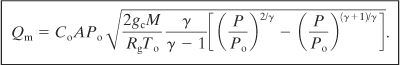
Equation 4-48 describes the mass flow rate at any point during the isentropic expansion.
For many safety studies the maximum flow rate of vapor through the hole is required. This is determined by differentiating Equation 4-48 with respect to P/Po and setting the derivative equal to zero. The result is solved for the pressure ratio resulting in the maximum flow:
(4-49)
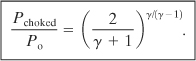
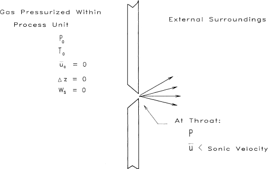
The choked pressure Pchoked is the maximum downstream pressure resulting in maximum flow through the hole or pipe. For downstream pressures less than Pchoked the following statements are valid: (1) The velocity of the fluid at the throat of the leak is the velocity of sound at the prevailing conditions, and (2) the velocity and mass flow rate cannot be increased further by reducing the downstream pressure; they are independent of the downstream conditions. This type of flow is called choked, critical, or sonic flow and is illustrated in Figure 4-10.
Figure 4-10 Choked flow of gas through a hole. The gas velocity is sonic at the throat. The mass flow rate is independent of the downstream pressure.
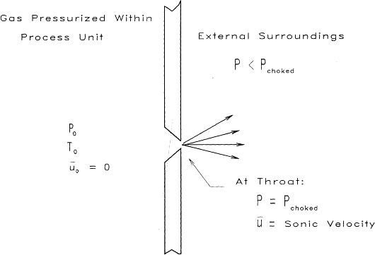
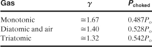
An interesting feature of Equation 4-49 is that for ideal gases the choked pressure is a function only of the heat capacity ratio γ. Thus:
For an air leak to atmospheric conditions (Pchoked = 14.7 psia), if the upstream pressure is greater than 14.7/0.528 = 27.8 psia, or 13.1 psig, the flow will be choked and maximized through the leak. Conditions leading to choked flow are common in the process industries.
The maximum flow is determined by substituting Equation 4-49 into Equation 4-48:
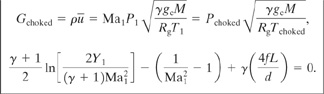
(4-50)
where
M is the molecular weight of the escaping vapor or gas,
To is the temperature of the source, and
Rg is the ideal gas constant.
For sharp-edged orifices with Reynolds numbers greater than 30,000 (and not choked), a constant discharge coefficient Co of 0.61 is indicated. However, for choked flows the discharge coefficient increases as the downstream pressure decreases.9 For these flows and for situations where Co is uncertain, a conservative value of 1.0 is recommended.
9Robert H. Perry and Cecil H. Chilton, Chemical Engineers Handbook, 7th ed. (New York: McGraw-Hill, 1997), pp. 10–16.
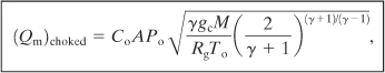
Values for the heat capacity ratio γ for a variety of gases are provided in Table 4-3.
Table 4-3 Heat Capacity Ratios γ for Selected Gases1
1Crane Co., Flow of Fluids Through Valves, Fittings, and Pipes, Technical Paper 410 (New York: Crane Co., 1986).
Example 4-4
A 0.1-in hole forms in a tank containing nitrogen at 200 psig and 80°F. Determine the mass flow rate through this leak.
Solution
From Table 4-3, for nitrogen γ = 1.41. Then from Equation 4-49
![]()
Thus
![]()
An external pressure less than 113.1 psia will result in choked flow through the leak. Because the external pressure is atmospheric in this case, choked flow is expected and Equation 4-50 applies. The area of the hole is
![]()
The discharge coefficient Co is assumed to be 1.0. Also,
Then, using Equation 4-50,
4-6 Flow of Gases through Pipes
Vapor flow through pipes is modeled using two special cases: adiabatic and isothermal behavior. The adiabatic case corresponds to rapid vapor flow through an insulated pipe. The isothermal case corresponds to flow through an uninsulated pipe maintained at a constant temperature; an underwater pipeline is an excellent example. Real vapor flows behave somewhere between the adiabatic and isothermal cases. Unfortunately, the real case is difficult to model and no generalized and useful equations are available.
For both the isothermal and adiabatic cases it is convenient to define a Mach (Ma) number as the ratio of the gas velocity to the velocity of sound in the gas at the prevailing conditions:
(4-51)
![]()
where a is the velocity of sound. The velocity of sound is determined using the thermodynamic relationship
(4-52)
![]()
which for an ideal gas is equivalent to
(4-53)
![]()
which demonstrates that for ideal gases the sonic velocity is a function of temperature only. For air at 20°C the velocity of sound is 344 m/s (1129 ft/s).
Adiabatic Flows
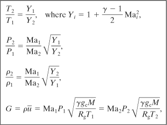
An adiabatic pipe containing a flowing vapor is shown in Figure 4-11. For this particular case the outlet velocity is less than the sonic velocity. The flow is driven by a pressure gradient across the pipe. As the gas flows through the pipe, it expands because of a decrease in pressure. This expansion leads to an increase in velocity and an increase in the kinetic energy of the gas. The kinetic energy is extracted from the thermal energy of the gas; a decrease in temperature occurs. However, frictional forces are present between the gas and the pipe wall. These frictional forces increase the temperature of the gas. Depending on the magnitude of the kinetic and frictional energy terms, either an increase or a decrease in the gas temperature is possible.
Figure 4-11 Adiabatic nonchoked flow of gas through a pipe. The gas temperature might increase or decrease, depending on the magnitude of the frictional losses.
The mechanical energy balance (Equation 4-1) also applies to adiabatic flows. For this case it is more conveniently written in the form
(4-54)
![]()
The following assumptions are valid for this case:
![]()
is valid for gases. Assuming a straight pipe without any valves or fittings, Equations 4-29 and 4-30 can be combined and then differentiated to result in
![]()
Because no mechanical linkages are present,
![]()
An important part of the frictional loss term is the assumption of a constant Fanning friction factor f across the length of the pipe. This assumption is valid only at high Reynolds numbers.
A total energy balance is useful for describing the temperature changes within the flowing gas. For this open steady flow process the total energy balance is given by
(4-55)
![]()
where h is the enthalpy of the gas and q is the heat. The following assumptions are invoked:
dh = C pdT for an ideal gas,
g/gcdz = 0 is valid for gases,
dq = 0 because the pipe is adiabatic,
dWs = 0 because no mechanical linkages are present.
These assumptions are applied to Equations 4-55 and 4-54. The equations are combined, integrated (between the initial point denoted by subscript “o” and any arbitrary final point), and manipulated to yield, after considerable effort,10
10Octave Levenspiel, Engineering Flow and Heat Exchange (New York: Plenum Press, 1986), p. 43.
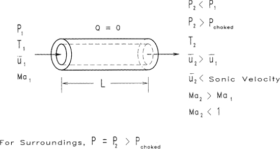
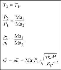
(4-56)
(4-57)
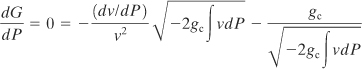
(4-58)
(4-59)
where G is the mass flux with units of mass/(area time) and
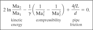
(4-60)
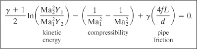
Equation 4-60 relates the Mach numbers to the frictional losses in the pipe. The various energy contributions are identified. The compressibility term accounts for the change in velocity resulting from the expansion of the gas.
Equations 4-59 and 4-60 are converted to a more convenient and useful form by replacing the Mach numbers with temperatures and pressures, using Equations 4-56 through 4-58:
(4-61)
(4-62)
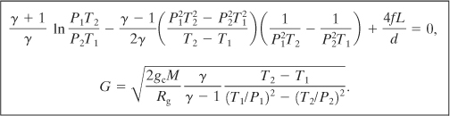
For most problems the pipe length (L), inside diameter (d), upstream temperature (T1) and pressure (P1), and downstream pressure (P2) are known. To compute the mass flux G, the procedure is as follows:
1. Determine pipe roughness ε from Table 4-1. Compute ε/d.
2. Determine the Fanning friction factor f from Equation 4-34. This assumes fully developed turbulent flow at high Reynolds numbers. This assumption can be checked later but is normally valid.
3. Determine T2 from Equation 4-61.
4. Compute the total mass flux G from Equation 4-62.
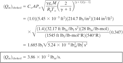
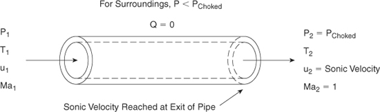
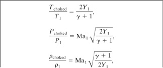
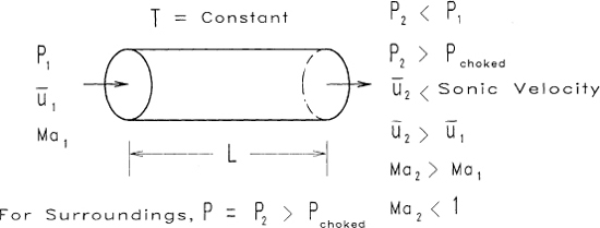
For long pipes or for large pressure differences across the pipe the velocity of the gas can approach the sonic velocity. This case is shown in Figure 4-12. When the sonic velocity is reached, the gas flow is called choked. The gas reaches the sonic velocity at the end of the pipe. If the upstream pressure is increased or if the downstream pressure is decreased, the gas velocity at the end of the pipe remains constant at the sonic velocity. If the downstream pressure is decreased below the choked pressure Pchoked, the flow through the pipe remains choked and constant, independent of the downstream pressure. The pressure at the end of the pipe will remain at Pchoked even if this pressure is greater than the ambient pressure. The gas exiting the pipe makes an abrupt change from Pchoked to the ambient pressure. For choked flow Equations 4-56 through 4-60 are simplified by setting Ma2 = 1.0. The results are
Figure 4-12 Adiabatic choked flow of gas through a pipe. The maximum velocity is reached at the end of the pipe.
(4-63)
(4-64)
(4-65)
(4-66)
(4-67)
Choked flow occurs if the downstream pressure is less than Pchoked. This is checked using Equation 4-64.
For most problems involving choked adiabatic flows the pipe length (L), inside diameter (d), and upstream pressure (P1) and temperature (T1) are known. To compute the mass flux G, the procedure is as follows:
1. Determine the Fanning friction factor f using Equation 4-34. This assumes fully developed turbulent flow at high Reynolds numbers. This assumption can be checked later but is normally valid.
2. Determine Ma1 from Equation 4-67.
3. Determine the mass flux Gchoked from Equation 4-66.
4. Determine Pchoked from Equation 5-64 to confirm operation at choked conditions.
Equations 4-63 through 4-67 for adiabatic pipe flow can be modified to use the 2-K method discussed previously by substituting Σ Kf for 4fL/d.
The procedure can be simplified by defining a gas expansion factor Yg. For ideal gas flow the mass flow for both sonic and nonsonic conditions is represented by the Darcy formula:11
11Crane Co., Flow of Fluids Thriugh Values, Fittings, and Pipes, Technical Report 410 (New York, Crane Co., 1986).
(4-68)
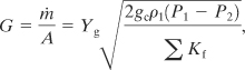
where
G is the mass flux (mass/area-time),
m is the mass flow rate of gas (mass/time),
A is the area of the discharge (length2),
Yg is a gas expansion factor (unitless),
gc is the gravitational constant (force/mass-acceleration),
ρ1 is the upstream gas density (mass/volume),
P1 is the upstream gas pressure (force/area),
P2 is the downstream gas pressure (force/area), and
ΣKf are the excess head loss terms, including pipe entrances and exits, pipe lengths, and fittings (unitless).
The excess head loss terms ∑ Kf are found using the 2-K method presented earlier in section 4-4. For most accidental discharges of gases the flow is fully developed turbulent flow. This means that for pipes the friction factor is independent of the Reynolds number and that for fittings Kf = K∞ and the solution is direct.
The gas expansion factor Yg in Equation 4-68 depends only on the heat capacity ratio of the gas γ and the frictional elements in the flow path ∑ Kf. An equation for the gas expansion factor for choked flow is obtained by equating Equation 4-68 to Equation 4-66 and solving for Yg. The result is
(4-69)
![]()
where Ma1 is the upstream Mach number.
The procedure to determine the gas expansion factor is as follows. First, the upstream Mach number Ma1 is determined using Equation 4-67. Kf must be substituted for 4fL/d to include the effects of pipes and fittings. The solution is obtained by trial and error, by guessing values of the upstream Mach number and determining whether the guessed value meets the equation objectives. This can be easily done using a spreadsheet.
The next step in the procedure is to determine the sonic pressure ratio. This is found from Equation 4-64. If the actual ratio is greater than the ratio from Equation 4-64, then the flow is sonic or choked and the pressure drop predicted by Equation 4-64 is used to continue the calculation. If less than the ratio from Equation 4-64, then the flow is not sonic and the actual pressure drop ratio is used.
Finally, the expansion factor Yg is calculated from Equation 4-69.
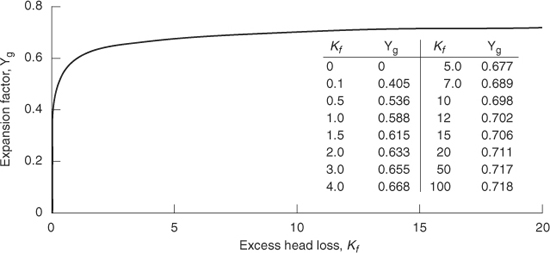
The calculation to determine the expansion factor can be completed once γ and the frictional loss terms ∑ Kf are specified. This computation can be done once and for all with the results shown in Figures 4-13 and 4-14. As shown in Figure 4-13, the pressure ratio (P1−P 2)/P1 is a weak function of the heat capacity ratio γ. The expansion factor Yg has little dependence on γ, with the value of Yg varying by less than 1% from the value at γ = 1.4 over the range from γ = 1.2 to γ = 1.67. Figure 4-14 shows the expansion factor for γ = 1.4.
Figure 4-13 Sonic pressure drop for adiabatic pipe flow for various heat capacity ratios. From AICHE/CCPS, Guidelines for Consequence Analysis of Chemical Releases (New York: American Institute of Chemical Engineers, 1999).
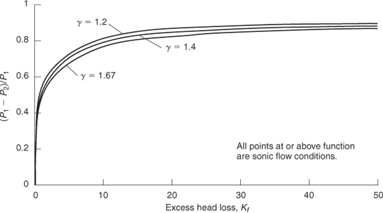
Figure 4-14 The expansion factor γ = Yg for adiabatic pipe flow for γ = 1.4. From AICHE/CCPS, Guidelines for Consequence Analysis of Chemical Releases (New York: American Institute of Chemical Engineers, 1999).
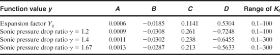
The functional results of Figures 4-13 and 4-14 can be fitted using an equation of the form ln Yg = A (ln Kf)3 + B (ln Kf)2 + C (ln Kf) + D, where A, B, C, and D are constants. The results are shown in Table 4-4 and are valid for the Kf ranges indicated, within 1%.
Table 4-4 Correlations1 for the Expansion Factor Yg, and the Sonic Pressure Drop Ratio (P1−P 2)/P1, as a Function of the Excess Head Loss Kf2
1The correlations are within 1% of the actual value in the specified range.
2The equation used to fit the expansion factor and the sonic pressure drop ratio is of the form
The procedure to determine the adiabatic mass flow rate through a pipe or hole is as follows:
1. Given: γ based on the type of gas; pipe length, diameter, and type; pipe entrances and exits; total number and type of fittings; total pressure drop; upstream gas density.
2. Assume fully developed turbulent flow to determine the friction factor for the pipe and the excess head loss terms for the fittings and pipe entrances and exits. The Reynolds number can be calculated at the completion of the calculation to check this assumption. Sum the individual excess head loss terms to get ∑ Kf.
ln Yg = A (ln Kf)3 + B (ln Kf)2 + C (ln Kf) 2 + D.
3. Calculate (P1 – P 2)/P1 from the specified pressure drop. Check this value against Figure 4-13 to determine whether the flow is sonic. All areas above the curves in Figure 4-13 represent sonic flow. Determine the sonic choking pressure P2 by using Figure 4-13 directly, interpolating a value from the table, or using the equations provided in Table 4-4.
4. Determine the expansion factor from Figure 4-14. Either read the value off of the figure, interpolate it from the table, or use the equation provided in Table 4-4.
5. Calculate the mass flow rate using Equation 4-68. Use the sonic choking pressure determined in step 3 in this expression.
This method is applicable to gas discharges through piping systems and holes.
Isothermal Flows
Isothermal flow of gas in a pipe with friction is shown in Figure 4-15. For this case the gas velocity is assumed to be well below the sonic velocity of the gas. A pressure gradient across the pipe provides the driving force for the gas transport. As the gas expands through the pressure gradient, the velocity must increase to maintain the same mass flow rate. The pressure at the end of the pipe is equal to the pressure of the surroundings. The temperature is constant across the entire pipe length.
Figure 4-15 Isothermal nonchoked flow of gas through a pipe.
Isothermal flow is represented by the mechanical energy balance in the form shown in Equation 4-54. The following assumptions are valid for this case:
![]()
is valid for gases, and, by combining Equations 4-29 and 4-30 and differentiating,
![]()
assuming constant f, and
δWs = 0
because no mechanical linkages are present. A total energy balance is not required because the temperature is constant.
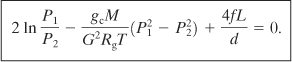
By applying the assumptions to Equation 4-54 and manipulating them considerably, we obtain 12
12Levenspiel, Engineering Flow, p. 46.
(4-70)
(4-71)
(4-72)
(4-73)
where G is the mass flux with units of mass/(area time), and
(4-74)
The various energy terms in Equation 4-74 have been identified.
A more convenient form of Equation 4-74 is in terms of pressure instead of Mach numbers. This form is achieved by using Equations 4-70 through 4-72. The result is
(4-75)
A typical problem is to determine the mass flux G given the pipe length (L), inside diameter (d), and upstream and downstream pressures (P1 and P2). The procedure is as follows:
1. Determine the Fanning friction factor f using Equation 4-34. This assumes fully developed turbulent flow at high Reynolds numbers. This assumption can be checked later but is usually valid.
2. Compute the mass flux G from Equation 4-75.
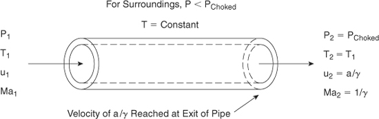
Levenspiel13 showed that the maximum velocity possible during the isothermal flow of gas in a pipe is not the sonic velocity, as in the adiabatic case. In terms of the Mach number the maximum velocity is
13Levenspiel, Engineering Flow, p. 46.
(4-76)
![]()
This result is shown by starting with the mechanical energy balance and rearranging it into the following form:
(4-77)
![]()
The quantity −(dP/dL)∞→ when Ma ∞ 1/![]() . Thus for choked flow in an isothermal pipe, as shown in Figure 4-16, the following equations apply:
. Thus for choked flow in an isothermal pipe, as shown in Figure 4-16, the following equations apply:
Figure 4-16 Isothermal choked flow of gas through a pipe. The maximum velocity is reached at the end of the pipe.
(4-78)
(4-79)
(4-80)
(4-81)
(4-82)
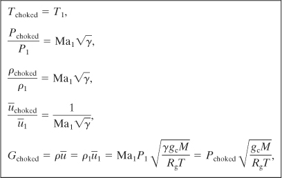
where Gchoked is the mass flux with units of mass/(area time), and
(4-83)
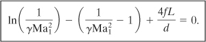
For most typical problems the pipe length (L), inside diameter (d), upstream pressure (P1), and temperature (T) are known. The mass flux G is determined using the following procedure:
1. Determine the Fanning friction factor using Equation 4-34. This assumes fully developed turbulent flow at high Reynolds numbers. This assumption can be checked later but is usually valid.
2. Determine Ma1 from Equation 4-83.
3. Determine the mass flux G from Equation 4-82.
For gas releases through pipes the issue of whether the release occurs adiabatically or isothermally is important. For both cases the velocity of the gas increases because of the expansion of the gas as the pressure decreases. For adiabatic flows the temperature of the gas may increase or decrease, depending on the relative magnitude of the frictional and kinetic energy terms. For choked flows the adiabatic choking pressure is less than the isothermal choking pressure. For real pipe flows from a source at a fixed pressure and temperature, the actual flow rate is less than the adiabatic prediction and greater than the isothermal prediction. Example 4-5 shows that for pipe flow problems the difference between the adiabatic and the isothermal results is generally small. Levenspiel14 showed that the adiabatic model always predicts a flow larger than the actual flow, provided that the source pressure and temperature are the same. The Crane Co.15 reported that “when compressible fluids discharge from the end of a reason ably short pipe of uniform cross-sectional area into an area of larger cross section, the flow is usually considered to be adiabatic.” Crane supported this statement with experimental data on pipes having lengths of 130 and 220 pipe diameters discharging air to the atmosphere. Finally, under choked sonic flow conditions isothermal conditions are difficult to achieve practically because of the rapid speed of the gas flow. As a result, the adiabatic flow model is the model of choice for compressible gas discharges through pipes.
14Levenspiel, Engineering Flow, p. 45.
15Crane Co., Flow of Fluids.
Example 4-5
The vapor space above liquid ethylene oxide (EO) in storage tanks must be purged of oxygen and then padded with 81-psig nitrogen to prevent explosion. The nitrogen in a particular facility is supplied from a 200-psig source. It is regulated to 81-psig and supplied to the storage vessel through 33 ft of commercial steel pipe with an internal diameter of 1.049 in.
In the event of a failure of the nitrogen regulator, the vessel will be exposed to the full 200-psig pressure from the nitrogen source. This will exceed the pressure rating of the storage vessel. To prevent rupture of the storage vessel, it must be equipped with a relief device to vent this nitrogen. Determine the required minimum mass flow rate of nitrogen through the relief device to prevent the pressure from rising within the tank in the event of a regulator failure.
Determine the mass flow rate assuming (a) an orifice with a throat diameter equal to the pipe diameter, (b) an adiabatic pipe, and (c) an isothermal pipe. Decide which result most closely corresponds to the real situation. Which mass flow rate should be used?
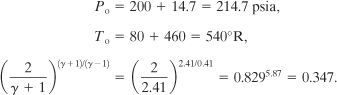
Solution.
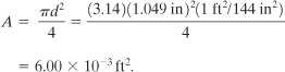
a. The maximum flow rate through the orifice occurs under choked conditions. The area of the pipe is
The absolute pressure of the nitrogen source is
Po = 200 + 14.7 = 214.7 psia = 3.09 × 10⁴ lbf/ft2.
The choked pressure from Equation 4-49 is, for a diatomic gas,
Pchoked = (0.528) (214.7 psia) = 113.4 psia
= 1.63 × 10⁴ lbf/ft2.
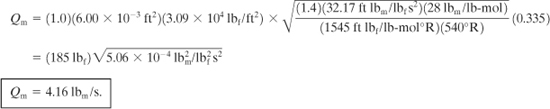
Choked flow can be expected because the system is venting to atmospheric conditions. Equation 4-50 provides the maximum mass flow rate. For nitrogen, γ = 1.4 and
![]()
The molecular weight of nitrogen is 28 lbm/lb-mol. Without any additional information, assume a unit discharge coefficient Co = 1.0. Thus
b. Assume adiabatic choked flow conditions. For commercial steel pipe, from Table 4-1, ε = 0.046 mm. The diameter of the pipe in millimeters is (1.049 in) (25.4 mm/in) = 26.6 mm. Thus
![]()
From Equation 4-34
For nitrogen, γ = 1.4.
The upstream Mach number is determined from Equation 4-67:
![]()
with Y1 given by Equation 4-56. Substituting the numbers provided gives
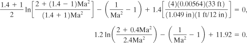
This equation is solved by trial and error for the value of Ma. The results are tabulated as follows:
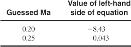
This last guessed Mach number gives a result close to zero. Then from Equation 4-56
![]()
and from Equations 4-63 and 4-64
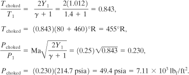
The pipe outlet pressure must be less than 49.4 psia to ensure choked flow. The mass flux is computed using Equation 4-66:
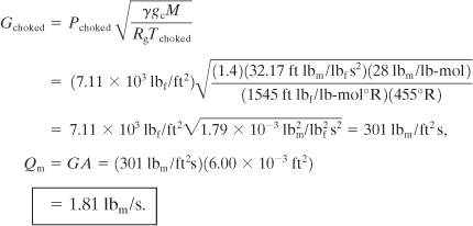
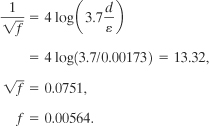
The simplified procedure with a direct solution can also be used. The excess head loss resulting from the pipe length is given by Equation 4-30. The friction factor f has already been determined:
![]()
For this solution only the pipe friction will be considered and the exit effects will be ignored. The first consideration is whether the flow is sonic. The sonic pressure ratio is given in Figure 4-13 (or the equations in Table 4-4). For γ = 1.4 and Kf = 8.56
![]()
It follows that the flow is sonic because the downstream pressure is less than 49.4 psia. From Figure 4-14 (or Table 4-4) the gas expansion factor Yg = 0.69. The gas density under the upstream conditions is
![]()
By substituting this value into Equation 4-68 and using the choking pressure determined for P2, we obtain
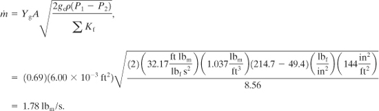
This result is essentially identical to the previous result, although with a lot less effort.
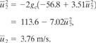
c. For the isothermal case the upstream Mach number is given by Equation 4-83. Substituting the numbers provided, we obtain
![]()
The solution is found by trial and error:
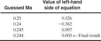
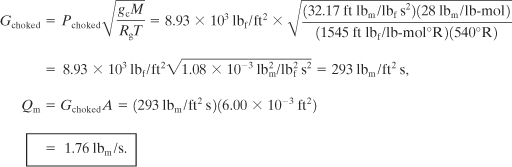
The choked pressure is, from Equation 4-79,
![]()
The mass flow rate is computed using Equation 4-82:
The results are summarized in the following table:
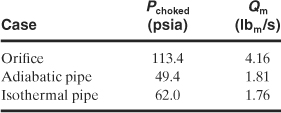
A standard procedure for these types of problems is to represent the discharge through the pipe as an orifice. The results show that this approach results in a large result for this case. The orifice method always produces a larger value than the adiabatic pipe method, ensuring a conservative safety design. The orifice calculation, however, is easier to apply, requiring only the pipe diameter and the upstream supply pressure and temperature. The configurational details of the piping are not required, as in the adiabatic and isothermal pipe methods.
Also note that the computed choked pressures differ for each case, with a substantial difference between the orifice and the adiabatic/isothermal cases. A choking design based on an orifice calculation might not be choked in reality because of high downstream pressures.
Finally, note that the adiabatic and isothermal pipe methods produce results that are reasonably close. For most real situations the heat transfer characteristics cannot be easily determined. Thus the adiabatic pipe method is the method of choice; it will always produce the larger number for a conservative safety design.
4-7 Flashing Liquids
Liquids stored under pressure above their normal boiling point temperature present substantial problems because of flashing. If the tank, pipe, or other containment device develops a leak, the liquid will partially flash into vapor, sometimes explosively.
Flashing occurs so rapidly that the process is assumed to be adiabatic. The excess energy contained in the superheated liquid vaporizes the liquid and lowers the temperature to the new boiling point. If m is the mass of original liquid, Cp the heat capacity of the liquid (energy/mass deg), To the temperature of the liquid before depressurization, and Tb the depressurized boiling point of the liquid, then the excess energy contained in the superheated liquid is given by
(4-84)
![]()
This energy vaporizes the liquid. If Δ Hv is the heat of vaporization of the liquid, the mass of liquid vaporized mv is given by
(4-85)
![]()
The fraction of the liquid vaporized is
(4-86)
Equation 4-86 assumes constant physical properties over the temperature range To to Tb. A more general expression without this assumption is derived as follows.
The change in liquid mass m resulting from a change in temperature T is given by
(4-87)
![]()
Equation 4-87 is integrated between the initial temperature To (with liquid mass m) and the final boiling point temperature Tb (with liquid mass m – mv):
(4-88)
![]()
(4-89)
![]()
where and ![]() ,
, ![]() are the mean heat capacity and the mean latent heat of vaporization, respectively, over the temperature range To to Tb. Solving for the fraction of the liquid vaporized, fv = mv/m, we obtain
are the mean heat capacity and the mean latent heat of vaporization, respectively, over the temperature range To to Tb. Solving for the fraction of the liquid vaporized, fv = mv/m, we obtain
(4-90)
![]()
Example 4-6
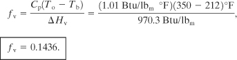
One lbm of saturated liquid water is contained in a vessel at 350°F. The vessel ruptures and the pressure is reduced to 1 atm. Compute the fraction of material vaporized using (a) the steam tables, (b) Equation 4-86, and (c) Equation 4-90.
Solution
a. The initial state is saturated liquid water at To = 350°F. From the steam tables
P = 134.6 psia,
H = 321.6 Btu/lbm.
The final temperature is the boiling point at 1 atm, or 212°F. At this temperature and under saturated conditions
Hvapor = 1150.4 Btu/lbm,
Hliquid = 180.07 Btu/lbm.
Because the process occurs adiabatically, Hfinal = Hinitial and the fraction of vapor (or quality) is computed from

that is, 14.59% of the mass of the original liquid is vaporized.
b. For liquid water at 212°F
Cp = 1.01 Btu/lbm °F,
ΔHv = 970.3 Btu/lbm.
From Equation 4-86
c. The mean properties for liquid water between To and Tb are
![]() = 1.04 Btu/ibm °F
= 1.04 Btu/ibm °F
![]() = 920.7 Btu/Ibm.
= 920.7 Btu/Ibm.
Substituting into Equation 4-90 gives
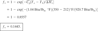
Both expressions work about as well compared to the actual value from the steam table.
For flashing liquids composed of many miscible substances, the flash calculation is complicated considerably, because the more volatile components flash preferentially. Procedures are available to solve this problem.16
16J. M. Smith and H. C. Van Ness, Introduction to Chemical Engineering Thermodynamics, 4th ed. (New York: McGraw-Hill, 1987), p. 314.
Flashing liquids escaping through holes and pipes require special consideration because two-phase flow conditions may be present. Several special cases need consideration.17 If the fluid path length of the release is short (through a hole in a thin-walled container), nonequi-librium conditions exist, and the liquid does not have time to flash within the hole; the fluid flashes external to the hole. The equations describing incompressible fluid flow through holes apply (see section 4-2).
17Hans K. Fauske, “Flashing Flows or: Some Practical Guidelines for Emergency Releases,” Plant/Operations Progress (July 1985), p. 133.
If the fluid path length through the release is greater than 10 cm (through a pipe or thick-walled container), equilibrium flashing conditions are achieved and the flow is choked. A good approximation is to assume a choked pressure equal to the saturation vapor pressure of the flashing liquid. The result will be valid only for liquids stored at a pressure higher than the saturation vapor pressure. With this assumption the mass flow rate is given by
(4-91)
![]()
where
A is the area of the release,
Co is the discharge coefficient (unitless),
ρf is the density of the liquid (mass/volume),
P is the pressure within the tank, and
Psat is the saturation vapor pressure of the flashing liquid at ambient temperature.
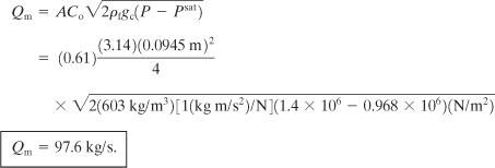
Example 4-7
Liquid ammonia is stored in a tank at 24°C and a pressure of 1.4 × 10⁶ Pa. A pipe of diameter 0.0945 m breaks off a short distance from the vessel (the tank), allowing the flashing ammonia to escape. The saturation vapor pressure of liquid ammonia at this temperature is 0.968 × 10⁶ Pa, and its density is 603 kg/m3. Determine the mass flow rate through the leak. Equilibrium flashing conditions can be assumed.
Solution
Equation 4-91 applies for the case of equilibrium flashing conditions. Assume a discharge coefficient of 0.61. Then
For liquids stored at their saturation vapor pressure, P = Psat, and Equation 4-91 is no longer valid. A much more detailed approach is required. Consider a fluid that is initially quiescent and is accelerated through the leak. Assume that kinetic energy is dominant and that potential energy effects are negligible. Then, from a mechanical energy balance (Equation 4-1), and realizing that the specific volume (with units of volume/mass) v = 1/ρ, we can write
(4-92)
![]()
A mass velocity G with units of mass/(area time) is defined by
(4-93)
![]()
Combining Equation 4-93 with Equation 4-92 and assuming that the mass velocity is constant results in
(4-94)
![]()
Solving for the mass velocity G and assuming that point 2 can be defined at any point along the flow path, we obtain
(4-95)
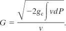
Equation 4-95 contains a maximum, at which choked flow occurs. Under choked flow conditions, dG/dP = 0. Differentiating Equation 4-95 and setting the result equal to zero gives
(4-96)
(4-97)
![]()
Solving Equation 4-97 for G, we obtain
(4-98)
The two-phase specific volume is given by
(4-99)
![]()
where
vfg is the difference in specific volume between vapor and liquid,
vf is the liquid specific volume, and
fv is the mass fraction of vapor.
Differentiating Equation 4-99 with respect to pressure gives
(4-100)
![]()
But, from Equation 4-86,
(4-101)
![]()
and from the Clausius-Clapyron equation, at saturation
(4-102)
![]()
Substituting Equations 4-102 and 4-101 into Equation 4-100 yields
(4-103)
![]()
The mass flow rate is determined by combining Equation 4-103 with Equation 4-98:
(4-104)
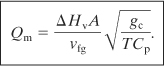
Note that the temperature T in Equation 4-104 is the absolute temperature from the Clausius-Clapyron equation and is not associated with the heat capacity.
Small droplets of liquid also form in a jet of flashing vapor. These aerosol droplets are readily entrained by the wind and transported away from the release site. The assumption that the quantity of droplets formed is equal to the amount of material flashed is frequently made.18
18Trevor A. Kletz, “Unconfined Vapor Cloud Explosions,” in Eleventh Loss Prevention Symposium (New York: American Institute of Chemical Engineers, 1977).
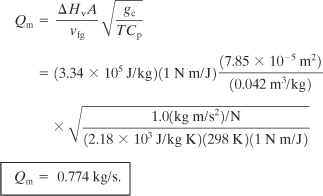
Example 4-8
Propylene is stored at 25°C in a tank at its saturation pressure. A 1-cm-diameter hole develops in the tank. Estimate the mass flow rate through the hole under these conditions for propylene:
ΔHv = 3.34 × 10⁵ J/kg,
vfg = 0.042 m3/kg,
Psat = 1.15 × 10⁶ Pa,
Cp = 2.18 × 10³ J/kg K.
Solution
Equation 4-104 applies to this case. The area of the leak is
![]()
Using Equation 4-104, we obtain
4-8 Liquid Pool Evaporation or Boiling
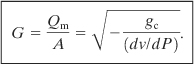
The case for evaporation of a volatile from a pool of liquid has already been considered in chapter 3. The total mass flow rate from the evaporating pool is given by Equation 3-12:
(3-12)
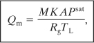
where
Qm is the mass vaporization rate (mass/time),
M is the molecular weight of the pure material,
K is the mass transfer coefficient (length/time),
A is the area of exposure,
Psat is the saturation vapor pressure of the liquid,
Rg is the ideal gas constant, and
TL is the temperature of the liquid.
For liquids boiling from a pool the boiling rate is limited by the heat transfer from the surroundings to the liquid in the pool. Heat is transferred (1) from the ground by conduction, (2) from the air by conduction and convection, and (3) by radiation from the sun and/or adjacent sources such as a fire.
The initial stage of boiling is usually controlled by the heat transfer from the ground. This is especially true for a spill of liquid with a normal boiling point below ambient temperature or ground temperature. The heat transfer from the ground is modeled with a simple one-dimensional heat conduction equation, given by
(4-105)
![]()
where
qg is the heat flux from the ground (energy/area-time),
ks is the thermal conductivity of the soil (energy/length-time-degree),
Tg is the temperature of the soil (degree),
T is the temperature of the liquid pool (degree),
αs is the thermal diffusivity of the soil (area/time), and
t is the time after spill (time).
Equation 4-105 is not considered conservative.
The rate of boiling is determined by assuming that all the heat is used to boil the liquid. Thus
(4-106)
![]()
where
Qm is the mass boiling rate (mass/time),
qg is the heat transfer for the pool from the ground, determined by Equation 4-105 (energy/area-time),
A is the area of the pool (area), and
Δ Hv is the heat of vaporization of the liquid in the pool (energy/mass).
At later times, solar heat fluxes and convective heat transfer from the atmosphere become important. For a spill onto an insulated dike floor these fluxes may be the only energy contributions. This approach seems to work adequately for liquefied natural gas (LNG) and perhaps for ethane and ethylene. The higher hydrocarbons (C3 and above) require a more detailed heat transfer mechanism. This model also neglects possible water freezing effects in the ground, which can significantly alter the heat transfer behavior. More details on boiling pools is provided elsewhere.19
19Guidelines for Consequence Analysis of Chemical Releases (1999).
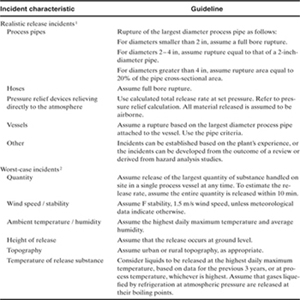
4-9 Realistic and Worst-Case Releases
Table 4-5 lists a number of realistic and worst-case releases. The realistic releases represent the incident outcomes with a high probability of occurring. Thus, rather than assuming that an entire storage vessel fails catastrophically, it is more realistic to assume that a high probability exists that the release will occur from the disconnection of the largest pipe connected to the tank.
Table 4-5 Guidelines for Selection of Process Incidents
1Dow’s Chemical Exposure Index Guide (New York: American Institute of Chemical Engineers, 1994).
2US EPA, RMP Offsite Consequence Analysis Guidance (Washington, DC: US Environmental Protection Agency, 1996).
The worst-case releases are those that assume almost catastrophic failure of the process, resulting in near instantaneous release of the entire process inventory or release over a short period of time.
The selection of the release case depends on the requirements of the consequence study. If an internal company study is being completed to determine the actual consequences of plant releases, then the realistic cases would be selected. However, if a study is being completed to meet the requirements of the EPA Risk Management Plan, then the worst-case releases must be used.
4-10 Conservative Analysis
All models, including consequence models, have uncertainties. These uncertainties arise because of (1) an incomplete understanding of the geometry of the release (that is, the hole size), (2) unknown or poorly characterized physical properties, (3) a poor understanding of the chemical or release process, and (4) unknown or poorly understood mixture behavior, to name a few.
Uncertainties that arise during the consequence modeling procedure are treated by assigning conservative values to some of these unknowns. By doing so, a conservative estimate of the consequence is obtained, defining the limits of the design envelope. This ensures that the resulting engineering design to mitigate or remove the hazard is overdesigned. Every effort, however, should be made to achieve a result consistent with the demands of the problem.
For any particular modeling study several receptors might be present that require different decisions for conservative design. For example, dispersion modeling based on a ground-level release will maximize the consequence for the surrounding community but will not maximize the consequence for plant workers at the top of a process structure.
To illustrate conservative modeling, consider a problem requiring an estimate of the gas discharge rate from a hole in a storage tank. This discharge rate is used to estimate the downwind concentrations of the gas, with the intent of estimating the toxicological impact. The discharge rate depends on a number of parameters, including (1) the hole area, (2) the pressure within and outside the tank, (3) the physical properties of the gas, and (4) the temperature of the gas, to name a few.
The reality of the situation is that the maximum discharge rate of gas occurs when the leak first occurs, with the discharge rate decreasing as a function of time as the pressure within the tank decreases. The complete dynamic solution to this problem is difficult, requiring a mass discharge model cross-coupled to a material balance on the contents of the tank. An equation of state (perhaps nonideal) is required to determine the tank pressure given the total mass. Complicated temperature effects are also possible. A modeling effort of this detail is not necessarily required to estimate the consequence.
A much simpler procedure is to calculate the mass discharge rate at the instant the leak occurs, assuming a fixed temperature and pressure within the tank equal to the initial temperature and pressure. The actual discharge rate at later times will always be less, and the down-wind concentrations will always be less. In this fashion a conservative result is ensured.
For the hole area a possible decision is to consider the area of the largest pipe connected to the tank, because pipe disconnections are a frequent source of tank leaks. Again, this maximizes the consequence and ensures a conservative result. This procedure is continued until all the model parameters are specified.
Unfortunately, this procedure can result in a consequence that is many times larger than the actual, leading to a potential overdesign of the mitigation procedures or safety systems. This occurs, in particular, if several decisions are made during the analysis, with each decision producing a maximum result. For this reason, consequence analysis should be approached with intelligence, tempered with a good dose of reality and common sense.
Suggested Reading
Consequence Modeling
AICHE/CCPS, Guidelines for Consequence Analysis of Chemical Releases (New York: American Institute of Chemical Engineers, 1999).
AICHE/CCPS, Guidelines for Chemical Process Quantitative Risk Analysis (New York: American Institute of Chemical Engineers, 2000).
Flow of Liquid through Holes
Frank P. Lees, Loss Prevention in the Process Industries, 2d ed. (London: Butterworths, 1996), p. 15/6.
Flow of Liquid through Pipes
Octave Levenspiel, Engineering Flow and Heat Exchange (New York: Plenum Press, 1984), ch. 2. Warren L. McCabe, Julian C. Smith, and Peter Harriott, Unit Operations of Chemical Engineering, 6th ed. (New York: McGraw-Hill, 2001), ch. 5.
Flow of Vapor through Holes
Lees, Loss Prevention, p. 15/10.
Levenspiel, Engineering Flow, pp. 48–51.
Flow of Vapor through Pipes
Levenspiel, Engineering Flow, ch. 3.
Flashing Liquids
Steven R. Hanna and Peter J. Drivas, Guidelines for Use of Vapor Dispersion Models, 2d ed. (New York: American Institute of Chemical Engineers, 1996), pp. 24–32.
Lees, Loss Prevention, p. 15/22.
Liquid Pool Evaporation and Boiling
Hanna and Drivas, Guidelines, pp. 31, 39.
Problems
4-1. A 0.20-in hole develops in a pipeline containing toluene. The pressure in the pipeline at the point of the leak is 100 psig. Determine the leakage rate. The specific gravity of toluene is 0.866.
4-2. A 100-ft-long horizontal pipeline transporting benzene develops a leak 43 ft from the high-pressure end. The diameter of the leak is estimated to be 0.1 in. At the time, the upstream pressure in the pipeline is 50 psig and the downstream pressure is 40 psig. Estimate the mass flow rate of benzene through the leak. The specific gravity of benzene is 0.8794.
4-3. The TLV-TWA for hydrogen sulfide gas is 10 ppm. Hydrogen sulfide gas is stored in a tank at 100 psig and 80°F. Estimate the diameter of a hole in the tank leading to a local hydrogen sulfide concentration equal to the TLV. The local ventilation rate is 2000 ft3/min and is deemed average. The ambient pressure is 1 atm.
4-4. A tank contains pressurized gas. Develop an equation describing the gas pressure as a function of time if the tank develops a leak. Assume choked flow and a constant tank gas temperature of To.
4-5. For incompressible flow in a horizontal pipe of constant diameter and without fittings or valves show that the pressure is a linear function of pipe length. What other assumptions are required for this result? Is this result valid for nonhorizontal pipes? How will the presence of fittings, valves, and other hardware affect this result?
4-6. A storage tank is 10 m high. At a particular time the liquid level is 5 m high within the tank. The tank is pressurized with nitrogen to 0.1 bar gauge to prevent a flammable atmosphere within the tank. The liquid in the tank has a density of 490 kg/m3.
a. If a 10-mm hole forms 3 m above the ground, what is the initial mass discharge rate of liquid (in kg/s)?
b. Estimate the distance from the tank the stream of liquid will hit the ground. Determine whether this stream will be contained by a 1-m-high dike located 1 m from the tank wall.
Hint: For a freely falling body the time to reach the ground is given by
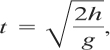
where t is the time, h is the initial height above the ground, and g is the acceleration due to gravity.
4-7. Water is pumped through a 1-in schedule 40 pipe (internal diameter = 1.049 in) at 400 gal/hr. If the pressure at one point in the pipe is 103 psig and a small leak develops 22 ft downstream, compute the fluid pressure at the leak. The pipe section is horizontal and without fittings or valves. For water at these conditions the viscosity is 1.0 centipoise and the density is 62.4 lbm/ft3.
4-8. If a globe valve is added to the pipe section of Problem 4-7, compute the pressure assuming that the valve is wide open.
4-9. A 31.5% hydrochloric acid solution is pumped from one storage tank to another. The power input to the pump is 2 kW and is 50% efficient. The pipe is plastic PVC pipe with an internal diameter of 50 mm. At a certain time the liquid level in the first tank is 4.1 m above the pipe outlet. Because of an accident, the pipe is severed between the pump and the second tank, at a point 2.1 m below the pipe outlet of the first tank. This point is 27 m in equivalent pipe length from the first tank. Compute the flow rate (in kg/s) from the leak. The viscosity of the solution is 1.8 × 10⁻³ kg/m s, and the density is 1600 kg/m3.
4-10. The morning inspection of the tank farm finds a leak in the turpentine tank. The leak is repaired. An investigation finds that the leak was 0.1 in in diameter and 7 ft above the tank bottom. Records show that the turpentine level in the tank was 17.3 ft before the leak occurred and 13.0 ft after the leak was repaired. The tank diameter is 15 ft. Determine (a) the total amount of turpentine spilled, (b) the maximum spill rate, and (c) the total time the leak was active. The density of turpentine at these conditions is 55 lb/ft3.
4-11. Compute the pressure in the pipe at the location shown on Figure 4-17. The flow rate through the pipe is 10,000 L/hr. The pipe is commercial steel pipe with an internal diameter of 50 mm. The liquid in the pipe is crude oil with a density of 928 kg/m3 and a viscosity of 0.004 kg/m s. The tank is vented to the atmosphere.
Figure 4-17 Process configuration for Problem 4-11.

4-12. A tank with a drain pipe is shown in Figure 4-18. The tank contains crude oil, and there is concern that the drain pipe might shear off below the tank, allowing the tank contents to leak out.
Figure 4-18 Tank draining process for Problem 4-12
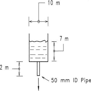
a. If the drain pipe shears 2 meters below the tank, and the oil level is 7 m at the time, estimate the initial mass flow rate of material out of the drain pipe.
b. If the pipe shears off at the tank bottom, leaving a 50-mm hole, estimate the initial mass flow rate.
The crude oil has a density of 928 kg/m3 and a viscosity of 0.004 kg/m s.
4-13. A cylinder in the laboratory contains nitrogen at 2200 psia. If the cylinder falls and the valve is sheared off, estimate the initial mass flow rate of nitrogen from the tank. Assume a hole diameter of 0.5 in. What is the force created by the jet of nitrogen?
4-14. A laboratory apparatus uses nitrogen at 250 psig. The nitrogen is supplied from a cylinder, through a regulator, to the apparatus through 15 ft of 0.25-in (internal diameter) drawn-copper tubing. If the tubing separates from the apparatus, estimate the flow of nitrogen from the tubing. The nitrogen in the tank is at 75°F.
4-15. Steam is supplied to the heating coils of a reactor vessel at 125 psig, saturated. The coils are 0.5-in schedule 80 pipe (internal diameter = 0.546 in). The steam is supplied from a main header through similar pipe with an equivalent length of 53 ft. The heating coils consist of 20 ft of the pipe wound in a coil within the reactor.
If the heating coil pipe shears accidently, the reactor vessel will be exposed to the full 125-psig pressure of the steam, exceeding the vessel’s pressure rating. As a result, the reactor must be equipped with a relief system to discharge the steam in the event of a coil shear. Compute the maximum mass flow rate of steam from the sheared coils using two approaches:
a. Assuming the leak in the coil is represented by an orifice.
b. Assuming adiabatic flow through the pipe.
4-16. A home hot water heater contains 40 gal of water. Because of a failure of the heat control, heat is continuously applied to the water in the tank, increasing the temperature and pressure. Unfortunately, the relief valve is clogged and the pressure rises past the maxi mum pressure of the vessel. At 250 psig the tank ruptures. Estimate the quantity of water flashed.
4-17. Calculate the mass flux (kg/m2 s) for the following tank leaks given that the storage pressure is equal to the vapor pressure at 25°C:
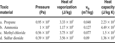
4-18. Large storage tanks need a breather vent (technically called a conservation vent) to allow air to move into and out of the tank as a result of temperature and pressure changes and a change in the tank liquid level. Unfortunately, these vents also allow volatile materials to escape, resulting in potential worker exposures.
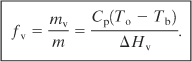
An expression that can be used to estimate the volatile emission rate in a storage tank resulting from a single change in temperature is given by
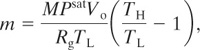
where m is the total mass of volatile released, M is the molecular weight of the volatile, Psat is the saturation vapor pressure of the liquid, Vo is the vapor volume of the tank, Rg is the ideal gas constant, TL is the initial low absolute temperature, and TH is the final absolute temperature.
A storage tank is 15 m in diameter and 10 m tall. It is currently half full of toluene (M = 92, Psat = 36.4 mm Hg). If the temperature changes from 4°C to 30°C over a period of 12 hr,
a. Derive the equation for m.
b. Estimate the rate of emission of toluene (in kg/s).
c. If a worker is standing near the vent, estimate the concentration (in ppm) of toluene in the air. Use an average temperature and an effective ventilation rate of 3000 ft3/min. Is the worker overexposed?
4-19. A tank 100 ft in diameter and 20 ft tall is filled with crude oil to within 2 ft of the top of the tank. One accident scenario is that a 6-in-diameter line connected to the bottom of the tank might break loose from the tank, allowing crude oil to drain out. If a 30-min emergency response time is required to stop the leak, estimate the maximum amount of crude oil (in gallons) leaked. The tank is vented to the atmosphere, and the specific gravity of crude oil is 0.9.
4-20. One accident mitigation procedure is called emergency material transfer, in which the material is transported away from the accident site before it becomes involved. We plan on mitigating a crude oil tank fire scenario by pumping the tank empty in 1 hr total time.
The crude oil storage tank is 30 m in diameter, and the crude oil is typically at a level of 9 m.
The transfer will be accomplished by pumping the crude oil through a 200-mm (internal diameter) commercial steel pipe to another tank 40 m in diameter and 10 m high. The pipeline represents 50 m of equivalent pipe.
a. Estimate the minimum pump size (in HP) required to pump the entire tank empty in 1 hr. Assume a pump efficiency of 80%.
b. If a 100-HP pump (80% efficient) is available, how long will it take to empty the tank?
c. What conclusions can be drawn about the viability of this approach?
The density of the crude oil is 928 kg/m3 with a viscosity of 0.004 kg/m s.
4-21. A storage tank contains water contaminated with a small quantity of a soluble hazardous waste material. The tank is 3 m in diameter and 6 m high. At the current time the liquid height is within 1 m of the top of the tank.
a. If a 3-cm (internal diameter) feed pipe at the bottom of the tank breaks off, how much liquid (in m3) is spilled if an emergency response procedure requires 30 min to stop the flow?
b. What is the final liquid level (in m)?
c. What is the maximum spill rate of liquid (in kg/s)?
Assume that the tank is vented.
4-22. A 3-cm (internal diameter) pipe has broken off of a 1-ton pig (or tank) of nitrogen. Estimate the maximum mass flow rate (in kg/s) of the gas if the initial pressure in the tank is 800 kPa gauge. The temperature is 25°C, and the ambient pressure is 1 atm.
4-23. A storage tank is vented to the atmosphere. If a hole develops in the tank, the liquid level hL is given by the following differential equation:
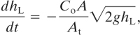
where hL is the liquid level height above the leak, Co is the constant discharge coefficient (=0.61), A is the cross-sectional area of the leak, At is the cross-sectional area of the tank, and g is the acceleration due to gravity.
a. Integrate the equation to determine an expression for the liquid level height as a function of time. Assume an initial liquid level above the leak of ![]() .
.
b. What is the driving force that pushes the water out of the hole in the tank?
c. If the cross-sectional area of the tank is increased, does the liquid level change faster, slower, or the same?
d. If the liquid level is increased, does the liquid level change faster, slower, or the same?
e. A cylindrical tank 10 ft high and 20 ft in diameter is used to store water. The liquid level in the tank is initially at 7 ft. If a 1-in puncture occurs 2 ft off the bottom of the tank, how long will it take for the water to drain down to the leak? What is the total amount of liquid (in gallons) discharged?
f. What would be the significance of the leak if the liquid were flammable? toxic?
4-24. Use a mechanical energy balance to show that the pump work required to pump a liquid through a pipe from one tank to another is given by
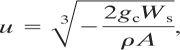
where Ws is the work input to the pump, f is the Fanning friction factor, L is the length of the pipe, ![]() is the mass flow rate, d is the diameter of the pipe, ρ is the density of the liquid, and A is the cross-sectional area of the pipe. Be sure to list clearly your assumptions!
is the mass flow rate, d is the diameter of the pipe, ρ is the density of the liquid, and A is the cross-sectional area of the pipe. Be sure to list clearly your assumptions!
4-25. In Example 4-5 the maximum flow through the nitrogen line was determined in order to size the relief device.
An important concept in process safety is inherent safety. This means that the process is designed in such a fashion as to prevent hazards from resulting in an accident.
Suppose that the reactor of Example 4-5 is equipped with a relief device capable of relieving nitrogen from the reactor vessel at the rate of 0.5 lbm/s. This is not enough to prevent overpressuring of the reactor in the event of a regulator failure. One inherently safer design method is to install an orifice in the nitrogen supply line to limit the flow of nitrogen.
a. Calculate the orifice diameter required to reduce the flow from the nitrogen line to 0.5 lbm/s.
b. What new safety or operational problems might arise as a result of installing the orifice?
4-26. A 10-m-diameter round tank sits on the ground within a 20-m-square diked area. The tank contains a hazardous material dissolved in mostly water. The tank is vented to the atmosphere.
A leak occurred in the tank because a 0.1-m-diameter pipe located 1 m above the bottom of the tank was accidentally disconnected. By the time the liquid flow was stopped, the liquid level in the diked area had reached a height of 0.79 m.
a. Estimate the total amount of liquid spilled (in m3 and in kg).
b. If the liquid level in the tank at the end of the spill was 8.5 m above the tank bottom, estimate the length of time for the leak.
c. What was the original liquid level in the tank?
4-27. a. Show that for any pump the maximum liquid discharge velocity is given by
where u is the maximum liquid discharge velocity, Ws is the pump shaft work, r is the density of the liquid, and A is the pump outlet discharge area. Make sure you list your assumptions in your solution.
b. A 1-kW pump discharges water through a 50-mm (internal diameter) pump outlet. What is the maximum velocity of the liquid from this pump? What is the maximum discharge rate (in kg/s)?
4-28. Consider an oil well drilled to a depth of 1000 ft and connected to the surface with 4-in (internal diameter) commercial steel pipe. If the pressure in the well reservoir is a constant 500 psig, what is the expected flow rate of liquid oil (in barrels per day) at the surface if the surface pipe is open to the atmosphere? Assume 1000 ft of equivalent pipe and no gas flow with the oil. The specific gravity of the oil is 0.93, and its viscosity is 0.4 centipoise. Make sure that you clearly state and justify any assumptions! Remember, an oil barrel is 42 gal.
4-29. Pumps can be blocked in by closing valves on the inlet and outlet sides of the pump. This can lead to a rapid increase in the temperature of the liquid blocked inside the pump.
A pump contains 4 kg of water. If the pump is rated at 1 HP, what is the maximum temperature increase expected in the water in °C/hr? Assume a constant heat capacity for the water of 1 kcal/kg°C. What will happen if the pump continues to operate?
4-30. Calculate the number of liters per year of liquid that can be transported through the following pipe sizes, assuming a constant liquid velocity of 1 m/s:
a. 3 cm internal diameter.
b. 5 cm internal diameter.
c. 25 cm internal diameter.
d. 50 cm internal diameter.
Comment on the magnitude of the result and the necessity for large pipe sizes in a chemical plant.
4-31. Calculate the number of kilograms per year of ideal gas that can be transported through the following pipe sizes, assuming a gas velocity of 3 m/s, a pressure of 689 kPa gauge, a temperature of 25°C, and a molecular weight of 44:
a. 3 cm internal diameter.
b. 5 cm internal diameter.
c. 25 cm internal diameter.
d. 50 cm internal diameter.
Comment on the magnitude of the result and the necessity for large pipe sizes in a chemical plant.
4-32. The strip chart in Figure 4-19 displays the history of a leak in a storage tank. No other pumping or filling operations occur during this time. The tank is 10 m high and 10 m in diameter, and it contains a liquid with a specific gravity of 0.9.
Figure 4-19 Strip chart data for Problem 4-32.
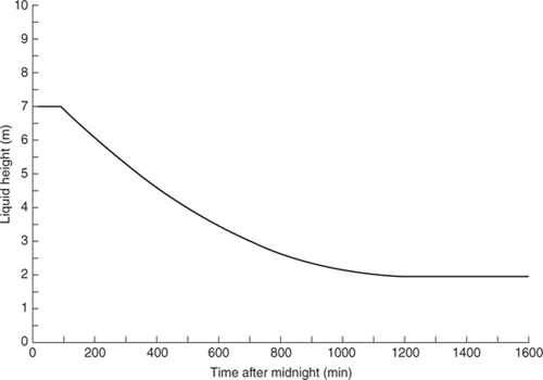
a. When did the leak start, and about how long did it last?
b. At what height is the leak?
c. What is the total quantity (in kg) leaked?
d. Estimate the maximum discharge rate of the fluid (in kg/s).
e. Estimate the leak hole diameter (in cm).
4-33. A storage vessel containing carbon tetrachloride (CCl4) is contained within a diked area with dimensions of 10 m × 10 m. The storage tank is in a horizontal bullet configuration with legs to raise the vessel well above the dike floor. The temperature of the liquid is 35°C, and the ambient pressure is 1 atm. The atomic weight of chlorine is 35.4.
a. What spill rate (in kg/s) from the storage vessel is required to completely fill the floor of the dike with liquid?
b. If one of the accident scenarios for this vessel results in a leak with a discharge rate of 1 kg/s, estimate the CCl4 vapor concentration near the vessel (in ppm), assuming an effective ventilation rate for the outdoors of 3000 ft3/min.
4-34. Show that for a spherical storage vessel containing liquid at an initial height ho the time for the liquid to drain from a hole in the bottom of the sphere is given by
where D is the inside diameter of the sphere, A is the area of the hole, Co is the discharge coefficient, and g is the acceleration due to gravity.
4-35. Estimate the vaporization rate resulting from heating from the ground at 10 s after the instantaneous spill of 1500 m3 of liquefied natural gas (LNG) into a rectangular concrete dike of dimensions 7 m by 10 m. You will need the following data:
Thermal diffusivity of soil: 4.16×10⁻⁷ m2/s
Thermal conductivity of soil: 0.92 W/m K
Temperature of liquid pool: 109 K
Temperature of soil: 293 K
Heat of vaporization of pool: 498 kJ/kg at 109 K