
Chapter 5 Toxic Release and Dispersion Models
During an accident, process equipment can release toxic materials quickly and in significant enough quantities to spread in dangerous clouds throughout a plant site and the local community. A few examples are explosive rupture of a process vessel as a result of excessive pressure caused by a runaway reaction, rupture of a pipeline containing toxic materials at high pressure, rupture of a tank containing toxic material stored above its atmospheric boiling point, and rupture of a train or truck transportation tank following an accident.
Serious accidents (such as Bhopal) emphasize the importance of planning for emergencies and of designing plants to minimize the occurrence and consequences of a toxic release. Toxic release models are routinely used to estimate the effects of a release on the plant and community environments.
An excellent safety program strives to identify problems before they occur. Chemical engineers must understand all aspects of toxic release to prevent the existence of release situations and to reduce the impact of a release if one occurs. This requires a toxic release model.
Toxic release and dispersion models are an important part of the consequence modeling procedure shown in Figure 4-1. The toxic release model represents the first three steps in the consequence modeling procedure. These steps are
1. identifying the release incident (what process situations can lead to a release? This was described in sections 4-9 and 4-10),
2. developing a source model to describe how materials are released and the rate of release (this was detailed in chapter 4), and
3. estimating the downwind concentrations of the toxic material using a dispersion model (once the downwind concentrations are known, several criteria are available to estimate the impact or effect, as discussed in section 5-4).
Various options are available, based on the predictions of the toxic release model, for example, (1) developing an emergency response plan with the surrounding community, (2) developing engineering modifications to eliminate the source of the release, (3) enclosing the potential release and adding appropriate vent scrubbers or other vapor removal equipment, (4) reducing inventories of hazardous materials to reduce the quantity released, and (5) adding area monitors to detect incipient leaks and providing block valves and engineering controls to eliminate hazardous levels of spills and leaks. These options are discussed in more detail in section 5-6 on release mitigation.
5-1 Parameters Affecting Dispersion
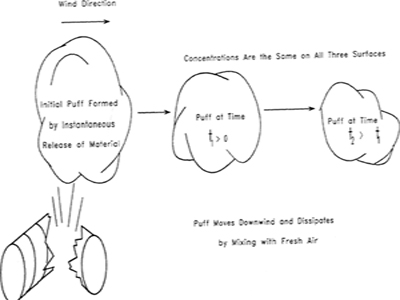
Dispersion models describe the airborne transport of toxic materials away from the accident site and into the plant and community. After a release the airborne toxic material is carried away by the wind in a characteristic plume, as shown in Figure 5-1, or a puff, as shown in Figure 5-2. The maximum concentration of toxic material occurs at the release point (which may not be at ground level). Concentrations downwind are less, because of turbulent mixing and dispersion of the toxic substance with air.
Figure 5-1 Characteristic plume formed by a continuous release of material.
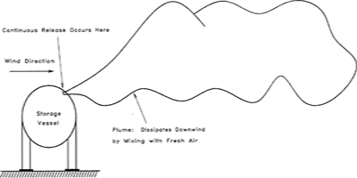
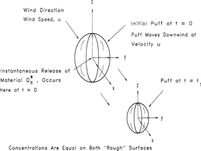
Figure 5-2 Puff formed by near instantaneous release of material.
A wide variety of parameters affect atmospheric dispersion of toxic materials:
• wind speed,
• atmospheric stability,
• ground conditions (buildings, water, trees),
• height of the release above ground level,
• momentum and buoyancy of the initial material released.
As the wind speed increases, the plume in Figure 5-1 becomes longer and narrower; the substance is carried downwind faster but is diluted faster by a larger quantity of air.
Atmospheric stability relates to vertical mixing of the air. During the day, the air temperature decreases rapidly with height, encouraging vertical motions. At night the temperature decrease is less, resulting in less vertical motion. Temperature profiles for day and night situations are shown in Figure 5-3. Sometimes an inversion occurs. During an inversion, the temperature increases with height, resulting in minimal vertical motion. This most often occurs at night because the ground cools rapidly as a result of thermal radiation.
Figure 5-3 Air temperature as a function of altitude for day and night conditions. The temperature gradient affects the vertical air motion. Adapted from D. Bruce Turner, Workbook of Atmospheric Dispersion Estimates (Cincinnati: US Department of Health, Education, and Welfare, 1970), p. 1.

Atmospheric stability is classified according to three stability classes: unstable, neutral, and stable. For unstable atmospheric conditions the sun heats the ground faster than the heat can be removed so that the air temperature near the ground is higher than the air temperature at higher elevations, as might be observed in the early morning hours. This results in unstable stability because air of lower density is below air of greater density. This influence of buoyancy enhances atmospheric mechanical turbulence. For neutral stability the air above the ground warms and the wind speed increases, reducing the effect of solar energy input, or insolation. The air temperature difference does not influence atmospheric mechanical turbulence. For stable atmospheric conditions the sun cannot heat the ground as fast as the ground cools; therefore the temperature near the ground is lower than the air temperature at higher elevations. This condition is stable because the air of higher density is below air of lower density. The influence of buoyancy suppresses mechanical turbulence.
Ground conditions affect the mechanical mixing at the surface and the wind profile with height. Trees and buildings increase mixing, whereas lakes and open areas decrease it. Figure 5-4 shows the change in wind speed versus height for a variety of surface conditions.
Figure 5-4 Effect of ground conditions on vertical wind gradient. Adapted from D. Bruce Turner, Workbook of Atmospheric Dispersion Estimates, (Cincinnati: US Department of Health, Education, and Welfare, 1970), p. 2.

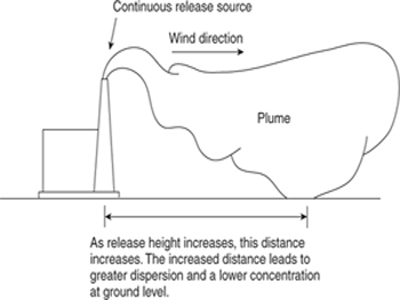
The release height significantly affects ground-level concentrations. As the release height increases, ground-level concentrations are reduced because the plume must disperse a greater distance vertically. This is shown in Figure 5-5.
Figure 5-5 Increased release height the ground concentration
The buoyancy and momentum of the material released change the effective height of the release. Figure 5-6 demonstrates these effects. The momentum of a high-velocity jet will carry the gas higher than the point of release, resulting in a much higher effective release height. If the gas has a density less than air, the released gas will initially be positively buoyant and will lift upward. If the gas has a density greater than air, then the released gas will initially be negatively buoyant and will slump toward the ground. The temperature and molecular weight of the released gas determine the gas density relative to that of air (with a molecular weight of 28.97). For all gases, as the gas travels downwind and is mixed with fresh air, a point will eventually be reached where the gas has been diluted adequately to be considered neutrally buoyant. At this point the dispersion is dominated by ambient turbulence.
Figure 5-6 The initial acceleration and buoyancy of the released material affects the plume character. The dispersion models discussed in this chapter represent only ambient turbulence. Adapted from Steven R. Hanna and Peter J. Drivas, Guidelines for Use of Vapor Cloud Dispersion Models (New York: American Institute of Chemical Engineers, 1987), p. 6.

5-2 Neutrally Buoyant Dispersion Models
Neutrally buoyant dispersion models are used to estimate the concentrations downwind of a release in which the gas is mixed with fresh air to the point that the resulting mixture is neutrally buoyant. Thus these models apply to gases at low concentrations, typically in the parts per million range.
Two types of neutrally buoyant vapor cloud dispersion models are commonly used: the plume and the puff models. The plume model describes the steady-state concentration of material released from a continuous source. The puff model describes the temporal concentration of material from a single release of a fixed amount of material. The distinction between the two models is shown graphically in Figures 5-1 and 5-2. For the plume model a typical example is the continuous release of gases from a smokestack. A steady-state plume is formed downwind from the smokestack. For the puff model a typical example is the sudden release of a fixed amount of material because of the rupture of a storage vessel. A large vapor cloud is formed that moves away from the rupture point.
The puff model can be used to describe a plume; a plume is simply the release of continuous puffs. However, if steady-state plume information is all that is required, the plume model is recommended because it is easier to use. For studies involving dynamic plumes (for instance, the effect on a plume of a change in wind direction), the puff model must be used.
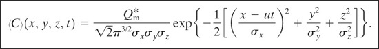
Consider the instantaneous release of a fixed mass of material, ![]() , into an infinite expanse of air (a ground surface will be added later). The coordinate system is fixed at the source. Assuming no reaction or molecular diffusion, the concentration C of material resulting from this release is given by the advection equation
, into an infinite expanse of air (a ground surface will be added later). The coordinate system is fixed at the source. Assuming no reaction or molecular diffusion, the concentration C of material resulting from this release is given by the advection equation
(5-1)
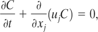
where uj is the velocity of the air and the subscript j represents the summation over all coordinate directions x, y, and z. If the velocity uj in Equation 5-1 is set equal to the average wind velocity and the equation is solved, we would find that the material disperses much faster than predicted. This is due to turbulence in the velocity field. If we could specify the wind velocity exactly with time and position, including the effects resulting from turbulence, Equation 5-1 would predict the correct concentration. Unfortunately, no models are currently available to adequately describe turbulence. As a result, an approximation is used. Let the velocity be represented by an average (or mean) and stochastic quantity
(5-2)
![]()
where
〈uj〉is the average velocity and ![]() is the stochastic fluctuation resulting from turbulence.
is the stochastic fluctuation resulting from turbulence.
It follows that the concentration C will also fluctuate as a result of the velocity field; so
(5-3)
![]()
where
〈C〉 is the mean concentration and
C′ is the stochastic fluctuation.
Because the fluctuations in both C and uj are around the average or mean values, it follows that
(5-4)

Substituting Equations 5-2 and 5-3 into Equation 5-1 and averaging the result over time yields
(5-5)
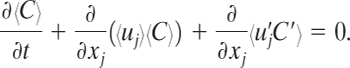
The terms 〈ujC′ and ![]() are zero when averaged (〈〈ujC′〉 = 〈uj〈C′〉 = 0), but the turbulent flux term
are zero when averaged (〈〈ujC′〉 = 〈uj〈C′〉 = 0), but the turbulent flux term ![]() is not necessarily zero and remains in the equation.
is not necessarily zero and remains in the equation.
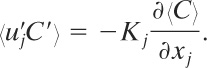
An additional equation is required to describe the turbulent flux. The usual approach is to define an eddy diffusivity Kj (with units of area/time) such that
(5-6)
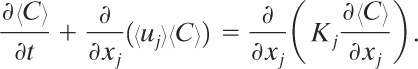
Substituting Equation 5-6 into Equation 5-5 yields
(5-7)
If the atmosphere is assumed to be incompressible, then
(5-8)

and Equation 5-7 becomes
(5-9)
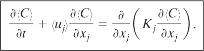
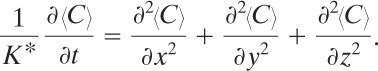
Equation 5-9 together with appropriate boundary and initial conditions forms the fundamental basis for dispersion modeling. This equation will be solved for a variety of cases.
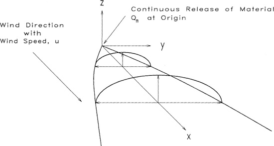
The coordinate system used for the dispersion models is shown in Figures 5-7 and 5-8. The x axis is the centerline directly downwind from the release point and is rotated for different wind directions. The y axis is the distance off the centerline, and the z axis is the elevation above the release point. The point (x, y, z) = (0, 0, 0) is at the release point. The coordinates (x, y, 0) are level with the release point, and the coordinates (x, 0, 0) are along the centerline, or x axis.
Figure 5-7 Steady-state continuous point source release with wind. Note the coordinate system: x is downwind direction, y is off-wind direction, and z is vertical direction.

Figure 5-8 Puff with wind. After the initial instantaneous release, the puff moves with the wind.
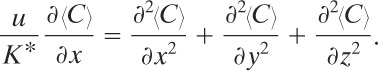
Case 1: Steady-State Continuous Point Release with No Wind
The applicable conditions are
• constant mass release rate (Qm = constant),
• no wind (〈uj〉 = 0)
• steady state (∂〈C/∂t = 0), and
• constant eddy diffusivity (Kj = K* in all directions).
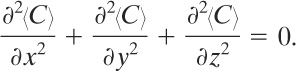
For this case Equation 5-9 reduces to the form
(5-10)
Equation 5-10 is more tractable by defining a radius as r2 = x2 + y2 + z 2. Transforming Equation 5-10 in terms of r yields
(5-11)

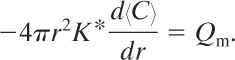
For a continuous steady-state release the concentration flux at any point r from the origin must equal the release rate Qm (with units of mass/time). This is represented mathematically by the following flux boundary condition:
(5-12)
The remaining boundary condition is
(5-13)
![]()
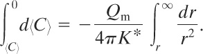
Equation 5-12 is separated and integrated between any point r and r = ∞:
(5-14)
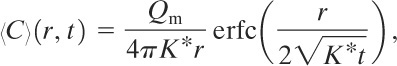
Solving Equation 5-14 for 〈C〉 yields
(5-15)

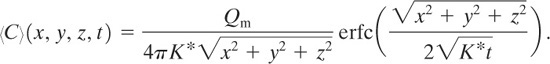
It is easy to verify by substitution that Equation 5-15 is also a solution to Equation 5-11 and thus a solution to this case. Equation 5-15 is transformed to rectangular coordinates to yield
(5-16)

Case 2: Puff with No Wind
The applicable conditions are
• puff release, that is, instantaneous release of a fixed mass of material ![]() (with units of mass),
(with units of mass),
• no wind (〈uj〉 = 0), and
• constant eddy diffusivity (Kj = K* in all directions).
Equation 5-9 reduces for this case to
(5-17)
The initial condition required to solve Equation 5-17 is
(5-18)
![]()
The solution to Equation 5-17 in spherical coordinates1 is
1H. S. Carslaw and J. C. Jaeger, Conduction of Heat in Solids (London: Oxford University Press, 1959), p. 256.
(5-19)

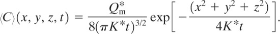
and in rectangular coordinates it is
(5-20)
Case 3: Non-Steady-State Continuous Point Release with No Wind
The applicable conditions are
• constant mass release rate (Qm = constant),
• no wind and (〈uj〉 = 0), and
• constant eddy diffusivity (Kj = K* in all directions).
For this case Equation 5-9 reduces to Equation 5-17 with the initial condition expressed by Equation 5-18 and the boundary condition expressed by Equation 5-13. The solution is found by integrating the instantaneous solution (Equation 5-19 or 5-20) with respect to time. The result in spherical coordinates2 is
2Carslaw and Jaeger, Conduction of Heat, p. 261.
(5-21)
and in rectangular coordinates it is
(5-22)
As t → ∞, Equations 5-21 and 5-22 reduce to the corresponding steady-state solutions (Equations 5-15 and 5-16).
Case 4: Steady-State Continuous Point Source Release with Wind
This case is shown in Figure 5-7. The applicable conditions are
• continuous release (Qm = constant),
• wind blowing in x direction only (〈uj〉 = 〈ux〉 = u = constant), and
• constant eddy diffusivity (Kj = K* in all directions).
For this case Equation 5-9 reduces to
(5-23)
Equation 5-23 is solved together with boundary conditions expressed by Equations 5-12 and 5-13. The solution for the average concentration at any point3 is
3Carslaw and Jaeger, Conduction of Heat, p. 267.
(5-24)

If a slender plume is assumed (the plume is long and slender and is not far removed from the x axis), that is,
(5-25)
![]()
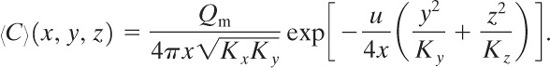
then by using ![]() , Equation 5-24 is simplified to
, Equation 5-24 is simplified to
(5-26)
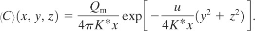
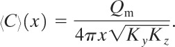
Along the centerline of this plume, y = z = 0, and
(5-27)

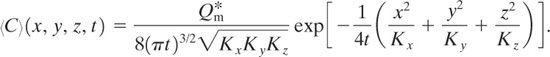
Case 5: Puff with No Wind and Eddy Diffusivity Is a Function of Direction
This case is the same as case 2 but with eddy diffusivity a function of direction. The applicable conditions are
• puff release (![]() = constant),
= constant),
• no wind and (〈uj = 0), and
• each coordinate direction has a different but constant eddy diffusivity (Kx, Ky, and Kz).
Equation 5-9 reduces to the following equation for this case:
(5-28)
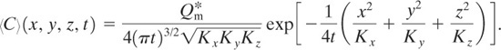
The solution is4
4Frank P. Lees, Loss Prevention in the Process Industries, 2d ed. (London: Butterworths, 1996), p. 15/106.
(5-29)
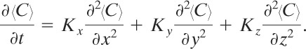
Case 6: Steady-State Continuous Point Source Release with Wind and Eddy Diffusivity Is a Function of Direction
This case is the same as case 4 but with eddy diffusivity a function of direction. The applicable conditions are
• continuous release (Qm = constant),
• steady-state (∂〈C〉/∂t = 0),
• wind blowing in x direction only (〈uj〉 = 〈ux〉 = u = constant),
• each coordinate direction has a different but constant eddy diffusivity (Kx, Ky, and Kz), and
• slender plume approximation (Equation 5-25).
Equation 5-9 reduces to
(5-30)

The solution is5
5Lees, Loss Prevention, p. 15/107.
(5-31)
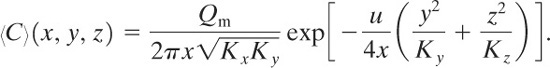
Along the centerline of this plume, y = z = 0, and the average concentration is given by
(5-32)
Case 7: Puff with Wind
This case is the same as case 5 but with wind. Figure 5-8 shows the geometry. The applicable conditions are
• puff release (![]() = constant),
= constant),
• wind blowing in x direction only (〈uj〉 = 〈ux〉 = u = constant), and
• each coordinate direction has a different but constant eddy diffusivity (Kx, Ky, and Kz).
The solution to this problem is found by a simple transformation of coordinates. The solution to case 5 represents a puff fixed around the release point. If the puff moves with the wind along the x axis, the solution to this case is found by replacing the existing coordinate x by a new coordinate system, x – ut , that moves with the wind velocity. The variable t is the time since the release of the puff, and u is the wind velocity. The solution is simply Equation 5-29, transformed into this new coordinate system:
(5-33)

Case 8: Puff with No Wind and with Source on Ground
This case is the same as case 5 but with the source on the ground. The ground represents an impervious boundary. As a result, the concentration is twice the concentration in case 5. The solution is 2 times Equation 5-29:
(5-34)
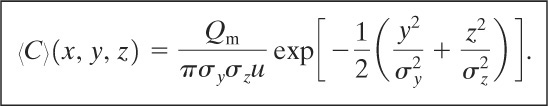
Case 9: Steady-State Plume with Source on Ground
This case is the same as case 6 but with the release source on the ground; as shown in Figure 5-9. The ground represents an impervious boundary. As a result, the concentration is twice the concentration in case 6. The solution is 2 times Equation 5-31:
Figure 5-9 Steady-state plume with source at ground level. The concentration is twice the concentration of a plume without the ground.
(5-35)
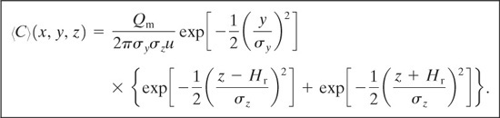
Case 10: Continuous Steady-State Source with Source at Height Hr above the Ground
For this case the ground acts as an impervious boundary at a distance H from the source. The solution is6
6Lees, Loss Prevention, p. 15/107.
(5-36)
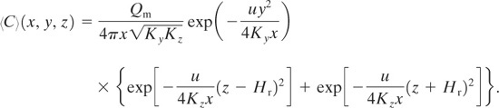
If Hr = 0, Equation 5-36 reduces to Equation 5-35 for a source on the ground.
Pasquill-Gifford Model
Cases 1 through 10 all depend on the specification of a value for the eddy diffusivity Kj. In general, Kj changes with position, time, wind velocity, and prevailing weather conditions. Although the eddy diffusivity approach is useful theoretically, it is not convenient experimentally and does not provide a useful framework for correlation.
Sutton7 solved this difficulty by proposing the following definition for a dispersion coefficient:
7O. G. Sutton, Micrometeorology (New York: McGraw-Hill, 1953), p. 286.
(5-37)
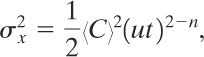
with similiar expressions given for σy and σz. The dispersion coefficients σx, σy, and σz represent the standard deviations of the concentration in the downwind, crosswind, and vertical (x, y, z) directions, respectively. Values for the dispersion coefficients are much easier to obtain experimentally than eddy diffusivities.
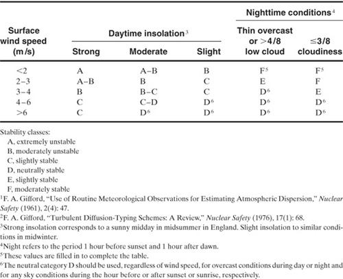
The dispersion coefficients are a function of atmospheric conditions and the distance downwind from the release. The atmospheric conditions are classified according to six different stability classes, shown in Table 5-1. The stability classes depend on wind speed and quantity of sunlight. During the day, increased wind speed results in greater atmospheric stability, whereas at night the reverse is true. This is due to a change in vertical temperature profiles from day to night.
Table 5-1 Atmospheric Stability Classes for Use with the Pasquill-Gifford Dispersion Model1,2
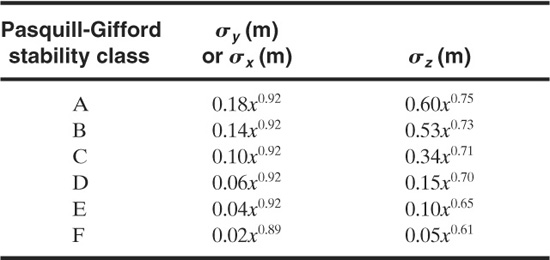
The dispersion coefficients σy and σz for a continuous source are given in Figures 5-10 and 5-11, with the corresponding correlations given in Table 5-2. Values for σx are not provided
Figure 5-10 Dispersion coefficients for Pasquill-Gifford plume model for rural releases.
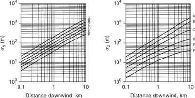
Figure 5-11 Dispersion coefficients for Pasquill-Gifford plume model for urban releases.
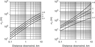
Table 5-2 Recommended Equations for Pasquill-Gifford Dispersion Coefficients for Plume Dispersion1,2 (the downwind distance x has units of meters)
A–F are defined in Table 5-1.
1R. F. Griffiths, “Errors in the Use of the Briggs Parameterization for Atmospheric Dispersion Coefficients,” Atmospheric Environment (1994), 28(17): 2861–2865.
2G. A. Briggs, Diffusion Estimation for Small Emissions, Report ATDL-106 (Washington, DC: Air Resources, Atmospheric Turbulence, and Diffusion Laboratory, Environmental Research Laboratories, 1974).
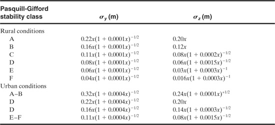
because it is reasonable to assume that σx = σy. The dispersion coefficients σy and σz for a puff release are given in Figure 5-12 and the equations are provided in Table 5-3. The puff dispersion coefficients are based on limited data (shown in Table 5-2) and should not be considered precise.
Figure 5-12 Dispersion coefficients for Pasquill-Gifford puff model.
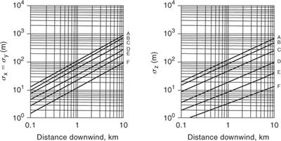
Table 5-3 Recommended Equations for Pasquill-Gifford Dispersion Coefficients for Puff Dispersion1,2 (the downwind distance x has units of meters)
A–F are defined in Table 5-1.
1R. F. Griffiths, “Errors in the Use of the Briggs Parameterization for Atmospheric Dispersion Coefficients,” Atmospheric Environment (1994), 28(17): 2861–2865.
2G. A. Briggs, Diffusion Estimation for Small Emissions, Report ATDL-106 (Washington, DC: Air Resources, Atmospheric Turbulence, and Diffusion Laboratory, Environmental Research Laboratories, 1974).
The equations for cases 1 through 10 were rederived by Pasquill8 using expressions of the form of Equation 5-37. These equations along with the correlations for the dispersion coefficients are known as the Pasquill-Gifford model.
8F. Pasquill, Atmospheric Diffusion (London: Van Nostrand, 1962).
Case 11: Puff with Instantaneous Point Source at Ground Level, Coordinates Fixed at Release Point, Constant Wind Only in x Direction with Constant Velocity u
This case is identical to case 7. The solution has a form similar to Equation 5-33:
(5-38)
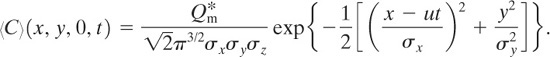
The ground-level concentration is given at z = 0:
(5-39)
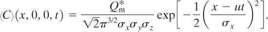
The ground-level concentration along the x axis is given at y = z = 0:
(5-40)
The center of the cloud is found at coordinates (ut, 0, 0). The concentration at the center of this moving cloud is given by
(5-41)

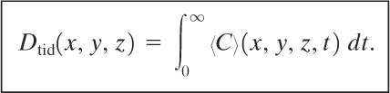
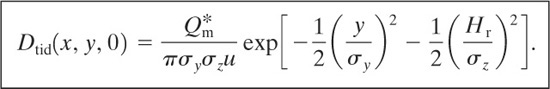
The total integrated dose Dtid received by an individual standing at fixed coordinates (x,y , z) is the time integral of the concentration:
(5-42)
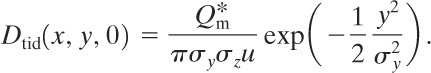
The total integrated dose at ground level is found by integrating Equation 5-39 according to Equation 5-42. The result is
(5-43)
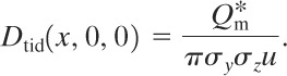
The total integrated dose along the x axis on the ground is
(5-44)
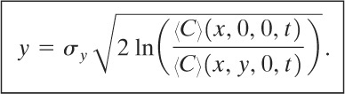
Frequently the cloud boundary defined by a fixed concentration is required. The line connecting points of equal concentration around the cloud boundary is called an isopleth. For a specified concentration 〈C〉* the isopleths at ground level are determined by dividing the equation for the centerline concentration (Equation 5-40) by the equation for the general ground-level concentration (Equation 5-39). This equation is solved directly for y:
(5-45)
The procedure is
1. Specify 〈C〉*, u, and t.
2. Determine the concentrations 〈C〉(x, 0, 0, t) along the x axis using Equation 5-40. Define the boundary of the cloud along the x axis.
3. Set 〈C〉(x, y, 0, t) = 〈C〉* in Equation 5-45, and determine the values of y at each center-line point determined in step 2.
The procedure is repeated for each value of t required.
Case 12: Plume with Continuous Steady-State Source at Ground Level and Wind Moving in x Direction at Constant Velocity u
This case is identical to case 9. The solution has a form similar to Equation 5-35:
(5-46)
The ground-level concentration is given at z = 0:
(5-47)

The concentration along the centerline of the plume directly downwind is given at y = z = 0:
(5-48)

The isopleths are found using a procedure identical to the isopleth procedure used for case 11.
For continuous ground-level releases the maximum concentration occurs at the release point.
Case 13: Plume with Continuous Steady-State Source at Height Hr above Ground Level and Wind Moving in x Direction at Constant Velocity u
This case is identical to case 10. The solution has a form similar to Equation 5-36:
(5-49)
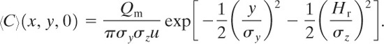
The ground-level concentration is found by setting z = 0:
(5-50)
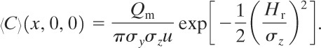
The ground-level centerline concentrations are found by setting y = z = 0:
(5-51)
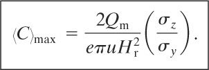
The maximum ground-level concentration along the x axis 〈C〉max is found using
(5-52)
The distance downwind at which the maximum ground-level concentration occurs is found from
(5-53)
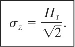
The procedure for finding the maximum concentration and the downwind distance is to use Equation 5-53 to determine the distance, followed by using Equation 5-52 to determine the maximum concentration.
Case 14: Puff with Instantaneous Point Source at Height Hr above Ground Level and a Coordinate System on the Ground That Moves with the Puff
For this case the center of the puff is found at x = ut. The average concentration is given by
(5-54)
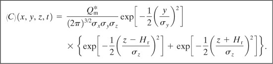
The time dependence is achieved through the dispersion coefficients, because their values change as the puff moves downwind from the release point. If wind is absent (u = 0), Equation 5-54 does not predict the correct result.
At ground level, z = 0, and the concentration is computed using
(5-55)

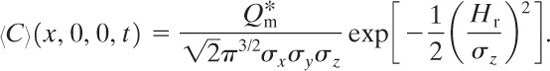
The concentration along the ground at the centerline is given at y = z = 0:
(5-56)
The total integrated dose at ground level is found by applying Equation 5-42 to Equation 5-55. The result is
(5-57)
Case 15: Puff with Instantaneous Point Source at Height Hr above Ground Level and a Coordinate System Fixed on the Ground at the Release Point
For this case the result is obtained using a transformation of coordinates similar to the transformation used for case 7. The result is
(5-58)

where t is the time since the release of the puff.
Worst-Case Conditions
For a plume the highest concentration is always found at the release point. If the release occurs above ground level, then the highest concentration on the ground is found at a point downwind from the release.
For a puff the maximum concentration is always found at the puff center. For a release above ground level the puff center will move parallel to the ground and the maximum concentration on the ground will occur directly below the puff center. For a puff isopleth the isopleth is close to circular as it moves downwind. The diameter of the isopleth increases initially as the puff travels downwind, reaches a maximum, and then decreases in diameter.
If weather conditions are not known or are not specified, then certain assumptions can be made to result in a worst-case result; that is, the highest concentration is estimated. The weather conditions in the Pasquill-Gifford dispersion equations are included by means of the dispersion coefficients and the wind speed. By examining the Pasguill-Gifford dispersion equations for estimating the concentrations, it is readily evident that the dispersion coefficients and wind speed are in the denominator. Thus the maximum concentration is estimated by selecting the weather conditions and wind speed that result in the smallest values of the dispersion coefficients and the wind speed. By inspecting Figures 5-10 through 5-12, we can see that the smallest dispersion coefficients occur with F stability. Clearly, the wind speed cannot be zero, so a finite value must be selected. The EPA9 suggests that F stability can exist with wind speeds as low as 1.5 m/s. Some risk analysts use a wind speed of 2 m/s. The assumptions used in the calculation must be clearly stated.
9EPA, RMP Offsite Consequence Analysis Guidance (Washington, DC: US Environmental Protection Agency, 1996).
Limitations to Pasquill-Gifford Dispersion Modeling
Pasquill-Gifford or Gaussian dispersion applies only to neutrally buoyant dispersion of gases in which the turbulent mixing is the dominant feature of the dispersion. It is typically valid only for a distance of 0.1–10 km from the release point.
The concentrations predicted by the Gaussian models are time averages. Thus it is possible for instantaneous local concentrations to exceed the average values predicted—this might be important for emergency response. The models presented here assume a 10-minute time average. Actual instantaneous concentrations may vary by as much as a factor of 2 from the concentrations computed using Gaussian models.
5-3 Dense Gas Dispersion
A dense gas is defined as any gas whose density is greater than the density of the ambient air through which it is being dispersed. This result can be due to a gas with a molecular weight greater than that of air or a gas with a low temperature resulting from autorefrigeration during release or other processes.
Following a typical puff release, a cloud having similar vertical and horizontal dimensions (near the source) may form. The dense cloud slumps toward the ground under the influence of gravity, increasing its diameter and reducing its height. Considerable initial dilution occurs because of the gravity-driven intrusion of the cloud into the ambient air. Subsequently the cloud height increases because of further entrainment of air across both the vertical and the horizontal interfaces. After sufficient dilution occurs, normal atmospheric turbulence predominates over gravitational forces and typical Gaussian dispersion characteristics are exhibited.
The Britter and McQuaid10 model was developed by performing a dimensional analysis and correlating existing data on dense cloud dispersion. The model is best suited for instantaneous or continuous ground-level releases of dense gases. The release is assumed to occur at ambient temperature and without aerosol or liquid droplet formation. Atmospheric stability was found to have little effect on the results and is not a part of the model. Most of the data came from dispersion tests in remote rural areas on mostly flat terrain. Thus the results are not applicable to areas where terrain effects are significant.
10R. E. Britter and J. McQuaid, Workbook on the Dispersion of Dense Gases (Sheffield, United Kingdom: Health and Safety Executive, 1988).
The model requires a specification of the initial cloud volume, the initial plume volume flux, the duration of release, and the initial gas density. Also required is the wind speed at a height of 10 m, the distance downwind, and the ambient gas density.
The first step is to determine whether the dense gas model is applicable. The initial cloud buoyancy is defined as
(5-59)
![]()
where
go is the initial buoyancy factor (length/time2),
g is the acceleration due to gravity (length/time2),
ρo is the initial density of released material (mass/volume), and
ρa is the density of ambient air (mass/volume).
A characteristic source dimension, dependent on the type of release, can also be defined. For continuous releases
(5-60)
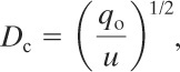
where
Dc is the characteristic source dimension for continuous releases of dense gases (length),
qo is the initial plume volume flux for dense gas dispersion (volume/time), and
u is the wind speed at 10 m elevation (length/time).
For instantaneous releases the characteristic source dimension is defined as
(5-61)
![]()
where
Di is the characteristic source dimension for instantaneous releases of dense gases (length) and
Vo is the initial volume of released dense gas material (length3).
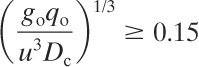
The criteria for a sufficiently dense cloud to require a dense cloud representation are, for continuous releases,
(5-62)
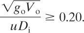
and, for instantaneous releases,
(5-63)
If these criteria are satisfied, then Figures 5-13 and 5-14 are used to estimate the downwind concentrations. Tables 5-4 and 5-5 provide equations for the correlations in these figures.
Figure 5-13 Britter-McQuaid dimensional correlation for dispersion of dense gas plumes.
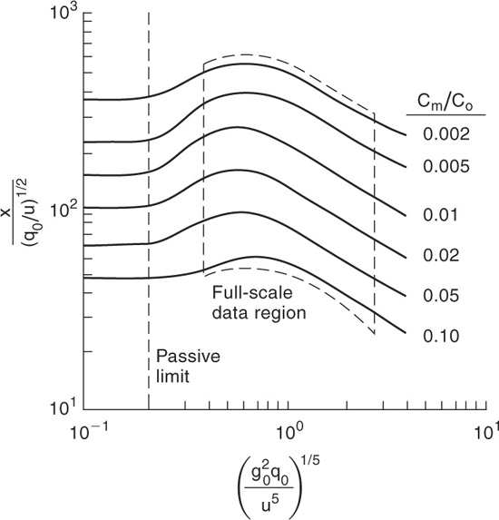
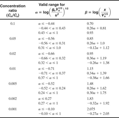
Figure 5-14 Britter-McQuaid dimensional correlation for dispersion of dense gas puffs.

Table 5-4 Equations Used to Approximate the Curves in the Britter-McQuaid Correlations Provided in Figure 5-13 for Plumes
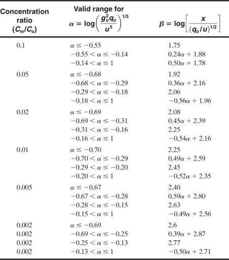
Table 5-5 Equations Used to Approximate the Curves in the Britter-McQuaid Correlations Provided in Figure 5-14 for Puffs
The criteria for determining whether the release is continuous or instantaneous is calculated using the following group:
(5-64)

where
Rd is the release duration (time) and
x is the downwind distance in dimensional space (length).
If this group has a value greater than or equal to 2.5, then the dense gas release is considered continuous. If the group value is less than or equal to 0.6, then the release is considered instantaneous. If the value lies in-between, then the concentrations are calculated using both continuous and instantaneous models and the maximum concentration result is selected.
For nonisothermal releases the Britter-McQuaid model recommends two slightly different calculations. For the first calculation a correction term is applied to the initial concentration (see Example 5-3). For the second calculation heat addition is assumed at the source to bring the source material to ambient temperature, which provides a limit to the effect of heat transfer. For gases lighter than air (such as methane or liquefied natural gas) the second calculation might be meaningless. If the difference between the two calculations is small, then the nonisothermal effects are assumed negligible. If the two calculations are within a factor of 2, then the calculation providing the maximum, or most pessimistic, concentration is used. If the difference is very large (greater than a factor of 2), then the maximum, or most pessimistic, concentration is selected, but further investigation using more detailed methods (such as a computer code) may be worthwhile.
The Britter-McQuaid model is a dimensional analysis technique, based on a correlation developed from experimental data. However, the model is based only on data from flat rural terrain and is applicable only to these types of releases. The model is also unable to account for the effects of parameters such as release height, ground roughness, and wind speed profiles.
5-4 Toxic Effect Criteria
Once the dispersion calculations are completed, the question arises: What concentration is considered dangerous? Concentrations based on TLV-TWA values, discussed in chapter 2, are overly conservative and are designed for worker exposures, not short-term exposures under emergency conditions.
One approach is to use the probit models developed in chapter 2. These models are also capable of including the effects resulting from transient changes in toxic concentrations. Unfortunately, published correlations are available for only a few chemicals, and the data show wide variations from the correlations.
One simplified approach is to specify a toxic concentration criterion above which it is assumed that individuals exposed to this value will be in danger. This approach has led to many criteria promulgated by several government agencies and private associations. Some of these criteria and methods include
• emergency response planning guidelines (ERPGs) for air contaminants issued by the American Industrial Hygiene Association (AIHA),
• IDLH levels established by NIOSH,
• emergency exposure guidance levels (EEGLs) and short-term public emergency guidance levels (SPEGLs) issued by the National Academy of Sciences/National Research Council,
• TLVs established by the ACGIH, including short-term exposure limits (TLV-STELs) and ceiling concentrations (TLV-Cs),
• PELs promulgated by OSHA,
• toxicity dispersion (TXDS) methods used by the New Jersey Department of Environmental Protection, and
• toxic endpoints promulgated by the EPA as part of the RMP.
These criteria and methods are based on a combination of results from animal experiments, observations of long- and short-term human exposures, and expert judgment. The following paragraphs define these criteria and describe some of their features.
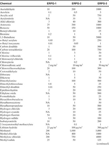
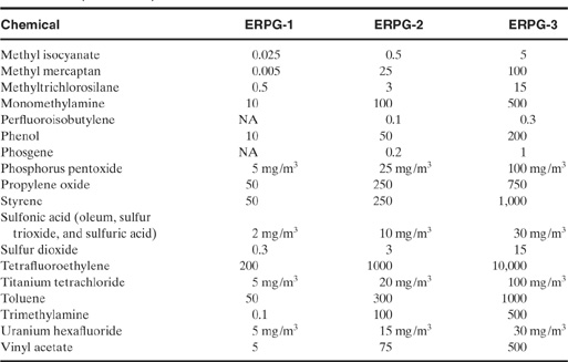
ERPGs are prepared by an industry task force and are published by the AIHA. Three concentration ranges are provided as a consequence of exposure to a specific substance:
1. ERPG-1 is the maximum airborne concentration below which it is believed nearly all individuals could be exposed for up to 1 hr without experiencing effects other than mild transient adverse health effects or perceiving a clearly defined objectionable odor.
2. ERPG-2 is the maximum airborne concentration below which it is believed nearly all individuals could be exposed for up to 1 hr without experiencing or developing irreversible or other serious health effects or symptoms that could impair their abilities to take protective action.
3. ERPG-3 is the maximum airborne concentration below which it is believed nearly all individuals could be exposed for up to 1 hr without experiencing or developing life-threatening health effects (similar to EEGLs).
ERPG data are shown in Table 5-6. To date, 47 ERPGs have been developed and are being reviewed, updated, and expanded by an AIHA peer review task force. Because of the comprehensive effort to develop acute toxicity values, ERPGs are becoming an acceptable industry/government norm.
Table 5-6 Emergency Response Planning Guidelines (ERPGs)1 (all values are in ppm unless otherwise noted)
1AIHA, Emergency Response Planning Guidelines and Workplace Environmental Exposure Levels (Fairfax, VA: American Industrial Hygiene Association, 1996).
NIOSH publishes IDLH concentrations to be used as acute toxicity measures for common industrial gases. An IDLH exposure condition is defined as a condition “that poses a threat of exposure to airborne contaminants when that exposure is likely to cause death or immediate or delayed permanent adverse health effects or prevent escape from such an environment.”11 IDLH values also take into consideration acute toxic reactions, such as severe eye irritation, that could prevent escape. The IDLH level is considered a maximum concentration above which only a highly reliable breathing apparatus providing maximum worker protection is permitted. If IDLH values are exceeded, all unprotected workers must leave the area immediately.
11NIOSH, NIOSH Pocket Guide to Chemical Hazards, Publication 94–116 (Washington, DC: US Department of Health and Human Services, 1994).
IDLH data are currently available for 380 materials. Because IDLH values were developed to protect healthy worker populations, they must be adjusted for sensitive populations, such as older, disabled, or ill populations. For flammable vapors the IDLH concentration is defined as one-tenth of the lower flammability limit (LFL) concentration. Also note that IDLH levels have not been peer-reviewed and that no substantive documentation for the values exists.
Since the 1940s, the National Research Council’s Committee on Toxicology has submitted EEGLs for 44 chemicals of special concern to the Department of Defense. An EEGL is defined as a concentration of a gas, vapor, or aerosol that is judged acceptable and that allows exposed individuals to perform specific tasks during emergency conditions lasting from 1 to 24 hr. Exposure to concentrations at the EEGL may produce transient irritation or central nervous system effects but should not produce effects that are lasting or that would impair performance of a task. In addition to EEGLs, the National Research Council has developed SPEGLs, defined as acceptable concentrations for exposures of members of the general public. SPEGLs are generally set at 10–50% of the EEGL and are calculated to take account of the effects of exposure on sensitive heterogeneous populations. The advantages of using EEGLs and SPEGLs rather than IDLH values are (1) a SPEGL considers effects on sensitive populations, (2) EEGLs and SPEGLs are developed for several different exposure durations, and (3) the methods by which EEGLs and SPEGLs were developed are well documented in National Research Council publications. EEGL and SPEGL values are shown in Table 5-7.
Table 5-7 Emergency Exposure Guidance Levels (EEGLs) from the National Research Council (NRC) (all values are in ppm unless otherwise noted)

Certain (ACGIH) criteria may be appropriate for use as benchmarks. The ACGIH threshold limit values—TLV-STELs and TLV-Cs—are designed to protect workers from acute effects resulting from exposure to chemicals; such effects include irritation and narcosis. These criteria are discussed in chapter 2. These criteria can be used for toxic gas dispersion but typically produce a conservative result because they are designed for worker exposures.
The PELs are promulgated by OSHA and have force of law. These levels are similar to the ACGIH criteria for TLV-TWAs because they are also based on 8-hr time-weighted average exposures. OSHA-cited “acceptable ceiling concentrations,” “excursion limits,” or “action levels” may be appropriate for use as benchmarks.
The New Jersey Department of Environmental Protection uses the TXDS method of consequence analysis to estimate potentially catastrophic quantities of toxic substances, as required by the New Jersey Toxic Catastrophe Prevention Act (TCPA). An acute toxic concentration (ATC) is defined as the concentration of a gas or vapor of a toxic substance that will result in acute health effects in the affected population and 1 fatality out of 20 or less (5% or more) during a 1-hr exposure. ATC values, as proposed by the New Jersey Department of Environmental Protection, are estimated for 103 “extraordinarily hazardous substances” and are based on the lowest value of one of the following: (1) the lowest reported lethal concentration (LCLO) value for animal test data, (2) the median lethal concentration (LC50) value from animal test data multiplied by 0.1, or (3) the IDLH value.
The EPA has promulgated a set of toxic endpoints to be used for air dispersion modeling for toxic gas releases as part of the EPA RMP.12 The toxic endpoint is, in order of preference, (1) the ERPG-2 or (2) the level of concern (LOC) promulgated by the Emergency Planning and Community Right-to-Know Act. The LOC is considered “the maximum concentration of an extremely hazardous substance in air that will not cause serious irreversible health effects in the general population when exposed to the substance for relatively short duration.” Toxic endpoints are provided for 74 chemicals under the RMP rule and are shown in Table 5-8.
12EPA, RMP Offsite Consequence Analysis Guidance (Washington, DC: US Environmental Protection Agency, 1996).
Table 5-8 Toxic Endpoints Specified by the EPA Risk Management Plan1
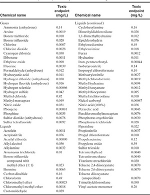
1EPA, RMP Offsite Consequence Analysis Guidance (Washington, DC: US Environmental Protection Agency, 1996).
In general, the most directly relevant toxicologic criteria currently available, particularly for developing emergency response plans, are ERPGs, SPEGLs, and EEGLs. These were developed specifically to apply to general populations and to account for sensitive populations and scientific uncertainty in toxicologic data. For incidents involving substances for which no SPEGLs or EEGLs are available, IDLH levels provide alternative criteria. However, because IDLH levels were not developed to account for sensitive populations and because they were based on a maximum 30-min exposure period, the EPA suggests that the identification of an effect zone should be based on exposure levels of one-tenth the IDLH level. For example, the IDLH level for chlorine dioxide is 5 ppm. Effect zones resulting from the release of this gas are defined as any zone in which the concentration of chlorine dioxide is estimated to exceed 0.5 ppm. Of course, the approach is conservative and gives unrealistic results; a more realistic approach is to use a constant-dose assumption for releases less than 30 min using the IDLH level.
The use of TLV-STELs and ceiling limits may be most appropriate if the objective is to identify effect zones in which the primary concerns include more transient effects, such as sensory irritation or odor perception. In general, persons located outside the zone that is based on these limits can be assumed to be unaffected by the release.
Craig et al.13 provided a hierarchy of alternative concentration guidelines in the event that ERPG data are not available. This hierarchy is shown in Table 5-9.
13D. K. Craig, J. S. Davis, R. DeVore, D. J. Hansen, A. J. Petrocchi, and T. J. Powell, “Alternative Guideline Limits for Chemicals without Environmental Response Planning Guidelines,” AIHA Journal (1995), 56.
Table 5-9 Recommended Hierarchy of Alternative Concentration Guidelines1
1D. K. Craig, J. S. Davis, R. DeVore, D. J. Hansen, A. J. Petrocchi, and T. J. Powell, “Alternative Guideline Limits for Chemicals without Environmental Response Planning Guidelines,” AIHA Journal (1995), 56.
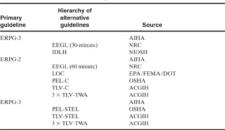
AIHA: American Industrial Hygiene Association
NIOSH: National Institute for Occupational Safety and Health
NRC: National Research Council Committee on Toxicology
EPA: Environmental Protection Agency
FEMA: Federal Emergency Management Agency
DOT: US Department of Transportation
OSHA: US Occupational Safety and Health Administration
ACGIH: American Conference of Governmental Industrial Hygienists
These methods may result in some inconsistencies because the different methods are based on different concepts. Good judgement should prevail.
Example 5-1
On an overcast day a stack with an effective height of 60 m is releasing sulfur dioxide at the rate of 80 g/s. The wind speed is 6 m/s. The stack is located in a rural area. Determine
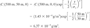
a. The mean concentration of SO2 on the ground 500 m downwind.
b. The mean concentration on the ground 500 m downwind and 50 m crosswind.
c. The location and value of the maximum mean concentration on ground level directly down-wind.
Solution
a. This is a continuous release. The ground concentration directly downwind is given by Equation 5-51:
(5-51)
![]()
From Table 5-1 the stability class is D.
The dispersion coefficients are obtained from either Figure 5-11 or Table 5-2. Using Table 5-2:
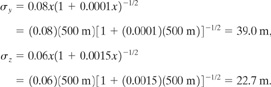
Substituting into Equation 5-51, we obtain

b. The mean concentration 50 m crosswind is found by using Equation 5-50 and by setting y = 50. The results from part a are applied directly:
c. The location of the maximum concentration is found from Equation 5-53:
![]()
From Figure 5-10 for D stability, σz has this value at about 1200 m downwind. From Figure 5-10 or Table 5-2, σy = 88 m. The maximum concentration is determined using Equation 5-52:
(5-52)

Example 5-2
Chlorine is used in a particular chemical process. A source model study indicates that for a particular accident scenario 1.0 kg of chlorine will be released instantaneously. The release will occur at ground level. A residential area is 500 m away from the chlorine source. Determine
a. The time required for the center of the cloud to reach the residential area. Assume a wind speed of 2 m/s.
b. The maximum concentration of chlorine in the residential area. Compare this with an ERPG-1 for chlorine of 1.0 ppm. What stability conditions and wind speed produces the maximum concentration?
c. Determine the distance the cloud must travel to disperse the cloud to a maximum concentration below the ERPG-1. Use the conditions of part b.
d. Determine the size of the cloud, based on the ERPG-1, at a point 5 km directly downwind on the ground. Assume the conditions of part b.
Assume in all cases that the chlorine cloud released is neutrally buoyant (which might not be a valid assumption).
Solution
a. For a distance of 500 m and a wind speed of 2 m/s, the time required for the center of the cloud to reach the residential area is
![]()
This leaves very little time for emergency warning.
b. The maximum concentration occurs at the center of the cloud directly downwind from the release. The concentration is given by Equation 5-41:
(5-41)
![]()
The stability conditions are selected to maximize in Equation 5-41. This requires dispersion coefficients of minimum value. From Figure 5-12 the lowest value of either dispersion coefficient occurs with F stability conditions. This is for nighttime conditions with thin to light overcast and a wind speed less than 3 m/s. The maximum concentration in the puff also occurs at the closest point to the release in the residential area. This occurs at a distance of 500 m. Thus
![]()
From Equation 5-41
![]()
This is converted to ppm using Equation 2-6. Assuming a pressure of 1 atm and a temperature of 298 K, the concentration in ppm is 798 ppm. This is much higher than the ERPG-1 of 1.0 ppm. Any individuals within the immediate residential area and any personnel within the plant will be excessively exposed if they are outside and downwind from the source.
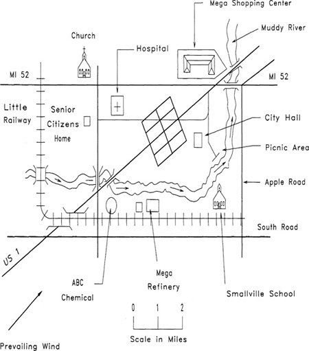
c. From Table 2-7 the ERPG-1 of 1.0 ppm is 3.0 mg/m3 or 3.0 X 10 6 kg/m3. The concentration at the center of the cloud is given by Equation 5-41. Substituting the known values, we obtain
The distance downwind is solved using the equations provided in Table 5-3. Thus for F stability
![]()
Solving for x by trial and error results in x = 8.0 km downwind.
d. The downwind centerline concentration is given by Equation 5-40:
(5-40)
![]()
The time required for the center of the plume to arrive is
![]()
At a downwind distance of x = 5 km = 5000 m and assuming F stability conditions, we calculate
![]()
Substituting the numbers provided gives
![]()
where x has units of meters. The quantity (x – 5000) represents the width of the plume. Solving for this quantity, we obtain

The cloud is 87.8 m wide at this point, based on the ERPG-1 concentration. At 2 m/s it will take approximately
![]()
to pass.
An appropriate emergency procedure would be to alert residents to stay indoors with the windows closed and ventilation off until the cloud passes. An effort by the plant to reduce the quantity of chlorine released is also indicated.
Example 5-314
14R. E. Britter and J. McQuaid, Workbook on the Dispersion of Dense Gases (Sheffield, United Kingdom: Health and Safety Executive, 1988).
Compute the distance downwind from the following liquefied natural gas (LNG) release to obtain a concentration equal to the lower flammability limit (LFL) of 5% vapor concentration by volume. Assume ambient conditions of 298 K and 1 atm. The following data are available:
Spill rate of liquid: 0.23 m3/s,
Spill duration (Rd): 174 s,
Wind speed at 10 m above ground (u): 10.9 m/s,
LNG density: 425.6 kg/m3,
LNG vapor density at boiling point of – 162°C: 1.76 kg/m3.
Solution
The volumetric discharge rate is given by
![]()
The ambient air density is computed from the ideal gas law and gives a result of 1.22 kg/m3. Thus from Equation 5-59:
![]()
Step 1. Determine whether the release is considered continuous or instantaneous. For this case expression 5-64 applies, and the quantity must be greater than 2.5 for a continuous release. Substituting the required numbers gives
![]()
and it follows that for a continuous release
![]()
The final distance must be less than this.
Step 2. Determine whether a dense cloud model applies. For this case Equations 5-60 and 5-62 apply. Substituting the appropriate numbers gives and it is clear that the dense cloud model applies.

Step 3. Adjust the concentration for a nonisothermal release. The Britter-MacQuaid model provides an adjustment to the concentration to account for nonisothermal release of the vapor. If the original concentration is C*, then the effective concentration is given by
![]()
where Ta is the ambient temperature and To is the source temperature, both in absolute temperature. For our required concentration of 0.05, the equation for C gives an effective concentration of 0.019.
Step 4. Compute the dimensionless groups for Figure 5-13:
![]()
and
![]()
Step 5. Apply Figure 5-13 to determine the downwind distance. The initial concentration of gas Co is essentially pure LNG. Thus Co = 1.0, and it follows that Cm/Co = 0.019. From Figure 5-13,
![]()
and it follows that x (2.26 m)(126) = 285 m. This compares to an experimentally determined distance of 200 m. This demonstrates that dense gas dispersion estimates can easily be off by a factor of 2.
5-5 Effect of Release Momentum and Buoyancy
Figure 5-6 indicates that the release characteristics of a puff or plume depend on the initial release momentum and buoyancy. The initial momentum and buoyancy change the effective height of release. A release that occurs at ground level but in an upward spouting jet of vaporizing liquid has a greater effective height than a release without a jet. Similarly, a release of vapor at a temperature higher than the ambient air temperature will rise because of buoyancy effects, increasing the effective height of the release.
Both effects are demonstrated by the traditional smokestack release shown in Figure 5-15. The material released from the smokestack contains momentum, based on its upward velocity within the stack pipe, and it is also buoyant, because its temperature is higher than the ambient temperature. Thus the material continues to rise after its release from the stack. The upward rise is slowed and eventually stopped as the released material cools and the momentum is dissipated.
Figure 5-15 Smokestack plume demonstrating initial buoyant rise of hot gases.

For smokestack releases Turner15 suggested using the empirical Holland formula to compute the additional height resulting from the buoyancy and momentum of the release:
15D. Bruce Turner, Workbook of Atmospheric Dispersion Estimates (Cincinnati: US Department of Health, Education, and Welfare, 1970), p. 31.
(5-65)
![]()
where
ΔHr is the correction to the release height Hr,
![]() s is the stack gas exit velocity (in m/s),
s is the stack gas exit velocity (in m/s),
d is the inside stack diameter (in m),
![]() is the wind speed (in m/s),
is the wind speed (in m/s),
P is the atmospheric pressure (in mb),
Ts is the stack gas temperature (in K), and
Ta is the air temperature (in K).
For heavier-than-air vapors, if the material is released above ground level, then the material will initially fall toward the ground until it disperses enough to reduce the cloud density.
5-6 Release Mitigation
The purpose of the toxic release model is to provide a tool for performing release mitigation. Release mitigation is defined as “lessening the risk of a release incident by acting on the source (at the point of release) either (1) in a preventive way by reducing the likelihood of an event that could generate a hazardous vapor cloud or (2) in a protective way by reducing the magnitude of the release and/or the exposure of local persons or property.”16
16Richard W. Prugh and Robert W. Johnson, Guidelines for Vapor Release Mitigation (New York: American Institute of Chemical Engineers, 1988), p. 2.
The release mitigation procedure is part of the consequence modeling procedure shown in Figure 4-1. After selection of a release incident, a source model is used to determine either the release rate or the total quantity released. This is coupled to a dispersion model and subsequent models for fires or explosions. Finally, an effect model is used to estimate the impact of the release, which is a measure of the consequence.
Risk is composed of both consequence and probability. Thus an estimate of the consequences of a release provides only half the total risk assessment. It is possible that a particular release incident might have high consequences, leading to extensive plant mitigation efforts to reduce the consequence. However, if the probability is low, the effort might not be required. Both the consequence and the probability must be included to assess risk.
Table 5-10 contains a number of measures to mitigate a release. The example problems presented in this chapter demonstrate that a small release can result in significant downwind impact. In addition, this impact can occur minutes after the initial release, reducing the time available for an emergency response procedure. Clearly, it is better to prevent the release in the first place. Inherent safety, engineering design, and management should be the first issues considered in any release mitigation procedure.
Table 5-10 Release Mitigation Approaches1
1Richard W. Prugh and Robert W. Johnson, Guidelines for Vapor Release Mitigation (New York: American Institute of Chemical Engineers, 1988).

Suggested Reading
Vapor Cloud Modeling
Guidelines for Consequence Analysis of Chemical Releases (New York: American Institute of Chemical Engineers, 1999).
Guidelines for Vapor Cloud Dispersion Models, 2d ed. (New York: American Institute of Chemical Engineers, 1996).
International Conference and Workshop on Modeling the Consequences of Accidental Releases of Hazardous Materials (New York: American Institute of Chemical Engineers, 1999).
Frank P. Lees, Loss Prevention in the Process Industries, 2d ed. (London: Butterworths, 1996), ch. 15 and 18.
John H. Seinfeld, Atmospheric Chemistry and Physics of Air Pollution (New York: Wiley, 1986), ch. 12, 13, and 14.
D. Bruce Turner, Workbook of Atmospheric Dispersion Estimates (Cincinnati: US Department of Health, Education, and Welfare, 1970).
Release Mitigation
Richard W. Prugh and Robert W. Johnson, Guidelines for Vapor Release Mitigation (New York: American Institute of Chemical Engineers, 1988).
Problems
5-1. A backyard barbeque grill contains a 20-lb tank of propane. The propane leaves the tank through a valve and regulator and is fed through a 1/2-in rubber hose to a dual valve assembly. After the valves the propane flows through a dual set of ejectors where it is mixed with air. The propane-air mixture then arrives at the burner assembly, where it is burned. Describe the possible propane release incidents for this equipment.
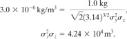
5-2. Contaminated toluene is fed to a water wash system shown in Figure 5-16. The toluene is pumped from a 50-gal drum into a countercurrent centrifugal extractor. The extractor separates the water from the toluene by centrifugal force acting on the difference in densities. The contaminated toluene enters the extractor at the periphery and flows to the center. The water enters the center of the extractor and flows to the periphery. The washed toluene and contaminated water flow into 50-gal drums. Determine a number of release incidents for this equipment.
Figure 5-16 Toluene water wash process.
5-3. A burning dump emits an estimated 3 g/s of oxides of nitrogen. What is the average concentration of oxides of nitrogen from this source directly downwind at a distance of 3 km on an overcast night with a wind speed of 7 m/s? Assume that this dump is a point ground-level source.
5-4. A trash incinerator has an effective stack height of 100 m. On a sunny day with a 2 m/s wind the concentration of sulfur dioxide 200 m directly downwind is measured at 5.0 × 10 5 g/m3. Estimate the mass release rate (in g/s) of sulfur dioxide from this stack. Also estimate the maximum sulfur dioxide concentration expected on the ground and its location downwind from the stack.
5-5. You have been suddenly enveloped by a plume of toxic material from a nearby chemical plant. Which way should you run with respect to the wind to minimize your exposure?
5-6. An air sampling station is located at an azimuth of 203° from a cement plant at a distance of 1500 m. The cement plant releases fine particulates (less than 15 μm diameter) at the rate of 750 lb/hr from a 30-m stack. What is the concentration of particulates at the air sampling station when the wind is from 30° at 3 m/s on a clear day in the late fall at 4:00 P.M.?
5-7. A storage tank containing acrolein (ERPG-1 = 0.1 ppm) is located 1500 m from a residential area. Estimate the amount of acrolein that must be instantaneously released at ground level to produce a concentration at the boundary of the residential area equal to the ERPG-1.
5-8. Consider again Problem 5-7, but assume a continuous release at ground level. What is the release rate required to produce an average concentration at the boundary to the residential area equal to the ERPG-1
5-9. The concentration of vinyl chloride 2 km downwind from a continuous release 25 m high is 1.6 mg/m3. It is a sunny day, and the wind speed is 18 km/hr. Determine the average concentration 0.1 km perpendicular to the plume 2 km downwind.
5-10. Diborane is used in silicon chip manufacture. One facility uses a 500-lb bottle. If the entire bottle is released continuously during a 20-min period, determine the location of the 5 mg/m3 ground-level isopleth. It is a clear, sunny day with a 5 mph wind. Assume that the release is at ground level.
5-11. Reconsider Problem 5-10. Assume now that the bottle ruptures and that the entire contents of diborane are released instantaneously. Determine, at 10 min after the release,
a. The location of the vapor cloud.
b. The location of the 5 mg/m3 isopleth.
c. The concentration at the center of the cloud.
d. The total dosage received by an individual standing on the downwind axis at the 15-min downwind location.
e. How far and long the cloud will need to travel to reduce the maximum concentration to 5 mg/m3.
5-12. An 800-lb tank of chlorine is stored at a water treatment plant. A study of the release scenarios indicates that the entire tank contents could be released as vapor in a period of 10 min. For chlorine gas, evacuation of the population must occur for areas where the vapor concentration exceeds the ERPG-1. Without any additional information, estimate the distance downwind that must be evacuated.
5-13. A reactor in a pesticide plant contains 1000 lb of a liquid mixture of 50% by weight liquid methyl isocyanate (MIC). The liquid is near its boiling point. A study of various release scenarios indicates that a rupture of the reactor will spill the liquid into a boiling pool on the ground. The boiling rate of MIC has been estimated to be 20 lb/min. Evacuation of the population must occur in areas where the vapor concentration exceeds ERPG-3. If the wind speed is 3.4 mph on a clear night, estimate the area downwind that must be evacuated.
5-14. A chemical plant has 10,000 lb of solid acrylamide stored in a large bin. About 20% by weight of the solid has a particle size less than 10 μm. A scenario study indicates that all the fine particles could be airborne in a period of 10 min. If evacuation must occur in areas where the particle concentration exceeds 110 mg/m3, estimate the area that must be evacuated.
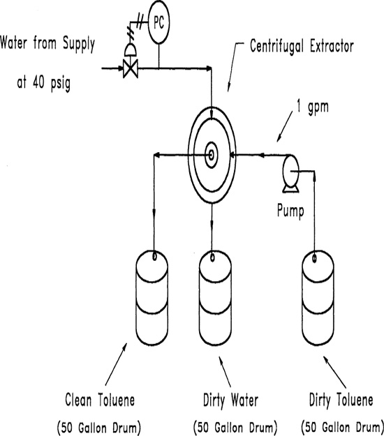
5-15. You have been appointed emergency coordinator for the community of Smallville, shown in Figure 5-17.
Figure 5-17 Map of Smallville.
ABC Chemical Company is shown on the map. They report the following chemicals and amounts: 100 lb of hydrogen chloride and 100 gal of sulfuric acid. You are required to develop an emergency plan for the community.
a. Determine which chemical presents the greater hazard to the community.
b. Assuming all of the chemical is released during a 10-min period, determine the distance downwind that must be evacuated.
c. Identify locations that might be affected by a release incident at the plant or might contribute to the incident because of its proximity to the plant.
d. Determine transportation routes that will be used to transport hazardous materials into or out of the facility. Identify any high-risk intersections where accidents might occur.
e. Determine the vulnerable zone along the transportation routes identified in part d. Use a distance of 0.5 mi on either side of the route, unless a smaller distance is indicated by part b.
f. Identify any special concerns (schools, nursing homes, shopping centers, and the like) that appear in the transportation route vulnerable zone.
g. Determine evacuation routes for the areas surrounding the plant.
h. Determine alternative traffic routes around the potential hazard.
i. Determine the resources required to support the needs of parts g and h.
j. Identify the means required to warn the area, and describe the content of an example warning message that could be used in an emergency at the facility.
k. Estimate the potential number of people evacuated during an emergency. Determine how these people are to be moved and where they might be evacuated to.
l. What other concerns might be important during a chemical emergency?
5-16. Derive Equation 5-43.
5-17. One response to a short-term release is to warn people to stay in their homes or offices with the windows closed and the ventilation off.
An average house, with the windows closed, exchanges air with the surroundings equal to three times the volume of the house per hour (although wide variations are expected).
a. Derive an equation for the concentration of chemical vapor within the house based on a parameter, Nt, equal to the number of volume exchanges per hour. Assume well-mixed behavior for the air, an initial zero concentration of vapor within the house, and a constant external concentration during the exposure period.
b. A vapor cloud with a maximum concentration of 20 ppm is moving through a community. Determine the time before the vapor concentration within an average house reaches 10 ppm.
c. If the wind is blowing at 2 mph and the plant is 1 mi upwind from the community, what is the maximum time available to the plant personnel to stop or reduce the release to ensure that the concentrations within the homes do not exceed the 10 ppm value?
5-18. A supply line (internal diameter = 0.493 in) containing chlorine gas is piped from a regulated supply at 50 psig. If the supply line ruptures, estimate the distance the plume must travel to reduce the concentration to 7.3 mg/m3. Assume an overcast day with a 15 mph wind and a temperature of 80°F. The release is near ground level.
5-19. A tank has ruptured and a pool of benzene has formed. The pool is approximately rectangular with dimensions of 20 ft by 30 ft. Estimate the evaporation rate and the distance affected downwind. Define the plume boundary using the TLV-TWA of 10 ppm. It is an overcast day with a 9 mph wind. The temperature is 90°F.
5-20. The EPA Risk Management Plan (RMP) defines a worst-case scenario as the catastrophic release of the entire process inventory in a 10-min period (assumed to be a continuous release). The dispersion calculations must be completed assuming F stability and 1.5 m/s wind speed. As part of the RMP rule, each facility must determine the downwind distance to a toxic endpoint. These results must be reported to the EPA and to the surrounding community.
a. A plant has a 100-lb tank of anhydrous hydrogen fluoride (molecular weight = 20). The toxic endpoint is specified in the RMP as 0.016 mg/L. Determine the distance down-wind (in miles) to the toxic endpoint for an EPA worst-case release.
b. Comment on the viability of using a continuous release model for a 10-min release period.
c. One hundred pounds of HF is a small quantity. Many plants have much larger vessels on site. Comment on how a larger quantity would affect the downwind distance and how this might affect the public’s perception of your facility. What does this imply about the size of chemical inventories for chemical plants?
5-21. A tank of chlorine contains 1000 kg of chlorine at 50 bar gauge (1 bar = 100,000 Pa). What is the maximum hole diameter (in mm) in this tank that will result in a downwind concentration equal to the ERPG-1 at a downwind distance of 300 m? Assume 1 atm, 25°C, a molecular weight of chlorine of 70.9, and that all the liquid chlorine vaporizes.
5-22. The emergency coordinator has decided that the appropriate emergency response to the immediate release of a toxic material is to alert people to stay in their homes, with doors and windows closed, until the cloud has passed. The coordinator has also indicated that homes 4000 m downwind must not be exposed to concentrations exceeding 0.10 mg/m3 of this material for any longer than 2 min. Estimate the maximum instantaneous release of material (in kg) allowed for these specifications. Be sure to clearly state any assumptions about weather conditions, wind speed, etc.
5-23. A tank containing hydrogen sulfide gas (molecular weight 34) has been overpressured and the relief device has been opened. In this case the relief device has a 3-cm diameter, and the flow through the relief is equivalent to the flow obtained through a 3-cm-diameter hole in the tank. In this case the flow of gas has been calculated to be 1.76 kg/s.
A cloud of material has formed downwind of the release. Determine the distance downwind that must be evacuated (in km). Assume that evacuation must occur in any location that exceeds the OSHA PEL. For this release the hydrogen sulfide in the tank is at a pressure of 1 MPa absolute and 25°C, the release occurs at ground level, and it is a clear night with a wind speed of 5.5 m/s.
5-24. A pipeline carrying benzene has developed a large leak. Fortunately, the leak occurred in a diked area and the liquid benzene is contained within the square 50 ft × 30 ft dike. The temperature is 80°F and the ambient pressure is 1 atm. It is a cloudy night with a 5 mph wind. All areas downwind with a concentration exceeding 4 times the PEL must be evacuated.
a. Determine the evaporation rate from the dike (in lb/s).
b. Determine the distance downwind (in mi) that must be evacuated.
c. Determine the maximum width of the plume (in ft) and the distance downwind (in mi) where it occurs.
5-25. You are developing emergency evacuation plans for the local community downwind of your plant. One scenario identified is the rupture of an ammonia pipeline. It is estimated that ammonia will release at the rate of 10 lb/s if this pipeline ruptures. You have decided that anyone exposed to more than 100 ppm of ammonia must be evacuated until repairs are made. What evacuation distance downwind will you recommend?
5-26. Emergency plans are being formulated so that rapid action can be taken in the event of an equipment failure. It is predicted that if a particular pipeline were to rupture, it would release ammonia at a rate of 100 lb/s. It is decided that anyone exposed to potential concentrations exceeding 500 ppm must be evacuated. What recommendation will you make as to the evacuation distance downwind? Assume that the wind speed is 6 mph and that the sun is shining brightly.
5-27. Use the Britter-McQuaid dense gas dispersion model to determine the distance to the 1% concentration for a release of chlorine gas. Assume that the release occurs over a duration of 500 s with a volumetric release rate of 1 m3/s. The wind speed at 10 m height is 10 m/s. The boiling point for the chlorine is –34°C, and the density of the liquid at the boiling point is 1470 kg/m3. Assume ambient conditions of 298 K and 1 atm.
5-28. Use a spreadsheet program to determine the location of a ground isopleth for a plume. The spreadsheet should have specific cell inputs for release rate (g/s), release height (m), spatial increment (m), wind speed (m/s), molecular weight of the released material, temperature (K), pressure (atm), and isopleth concentration (ppm).
The spreadsheet output should include, at each point downwind, both y and z dispersion coefficients (m), downwind centerline concentrations (ppm), and isopleth locations (m).
The spreadsheet should also have cells providing the downwind distance, the total area of the plume, and the maximum width of the plume, all based on the isopleth values.
Your submitted work should include a brief description of your method of solution, outputs from the spreadsheet, and plots of the isopleth locations.
Use the following two cases for computations, and assume worst-case stability conditions:
Case a: |
Release rate: 200 g/s |
|
Release height: 0 m |
|
Molecular weight: 100 |
|
Temperature: 298 K |
|
Pressure: 1 atm |
|
Isopleth concentration: 10 ppm |
Case b: |
Same as above, but release height = 10 m. Compare the plume width, area, and downwind distance for each case. Comment on the difference between the two cases. |
5-29. Develop a spreadsheet to determine the isopleths for a puff at a specified time after the release of material.
The spreadsheet should contain specific cells for user input of the following quantities: time after release (s), wind speed (2 m/s), total release (kg), release height (m), molecular weight of released gas, ambient temperature (K), ambient pressure (atm), and isopleth concentration (ppm).
The spreadsheet output should include, at each point downwind, downwind location, both y and z dispersion coefficients, downwind centerline concentration, and isopleth distance off-center (+/–).
The spreadsheet output should also include a graph of the isopleth location.
For your spreadsheet construction, we suggest that you set up the cells to move with the puff center. Otherwise, you will need a large number of cells.
Use the spreadsheet for the following case:
Release mass: 0.5 kg
Release height: 0 m
Molecular weight of gas: 30
Ambient temperature: 298 K
Ambient pressure: 1 atm
Isopleth concentration: 1 ppm
Atmospheric stability: F
Run the spreadsheet for a number of different times, and plot the maximum puff width as a function of distance downwind from the release.
Answer the following questions:
a. At what distance downwind does the puff reach its maximum width?
b. At what distance and time does the puff dissipate?
c. Estimate the total area swept out by the puff from initial release to dissipation.
Your submitted work should include a description of your method of solution, a complete spreadsheet output at 2000 s after release, a plot of maximum puff width as a function of downwind distance, and the calculation of the total swept area.
5-30. A fixed mass of toxic gas has been released almost instantaneously from a process unit. You have been asked to determine the percentage of fatalities expected 2000 m down-wind from the release. Prepare a spreadsheet to calculate the concentration profile around the center of the puff 2000 m downwind from the release. Use the total release quantity as a parameter. Determine the percentage of fatalities at the 2000-m downwind location as a result of the passing puff. Vary the total release quantity to result in a range of fatalities from 0 to 100%. Record the results at enough points to provide an accurate plot of the percentage of fatalities vs. quantity released. The release occurs at night with calm and clear conditions.
Change the concentration exponent value to 2.00 instead of 2.75 in the probit equation, and rerun your spreadsheet for a total release amount of 5 kg. How sensitive are the results to this exponent?
Hint: Assume that the puff shape and concentration profile remain essentially fixed as the puff passes.
Supplemental information:
Molecular weight of gas: 30
Temperature: 298 K
Pressure: 1 atm
Release height: 0
Wind speed: 2 m/s
Use a probit equation for fatalities of the form
![]()
where Y is the probit variable, C is the concentration in ppm, and T is the time interval (min).
Your submitted work must include a single output of the spreadsheet for a total release of 5 kg, including the puff concentration profile and the percent fatalities; a plot of the concentration profile for the 5-kg case vs. the distance in meters from the center of the puff; a plot of the percentage of fatalities vs. total quantity released; a single output of the spreadsheet for a 5-kg release with a probit exponent of 2.00; and a complete discussion of your method and your results.
5-31. A particular release of chlorine gas has resulted in the concentration profile given in Figure 5-18 for the cloud moving downwind along the ground. This is the concentration recorded at a fixed location as the cloud passes. The concentration increases linearly to a maximum concentration Cmax and then decreases linearly to zero.
Figure 5-18 Concentration profile for a chlorine gas release.
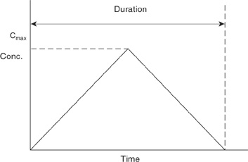
The width of the cloud is represented by the duration or time to pass, as shown. Develop a spreadsheet to compute the percentage of fatalities expected as a result of this cloud, with this particular shape, passing a fixed location. Set up your spreadsheet to include input parameters of cloud duration and maximum concentration. Use your spreadsheet to draw a plot of the percentage of fatalities vs. duration of exposure. Draw a curve on the plot for each of the maximum concentrations of 40, 50, 60, 70, 80, and 100 ppm. What conclusions can be drawn about the results?