Chapter 2
Toxicology
Because of the quantity and variety of chemicals used by the chemical process industries, chemical engineers must be knowledgeable about
• the way toxicants enter biological organisms,
• the way toxicants are eliminated from biological organisms,
• the effects of toxicants on biological organisms, and
• methods to prevent or reduce the entry of toxicants into biological organisms.
The first three areas are related to toxicology. The last area is essentially industrial hygiene, a topic considered in chapter 3.
Many years ago, toxicology was defined as the science of poisons. Unfortunately, the word poison could not be defined adequately. Paracelsus, an early investigator of toxicology during the 1500s, stated the problem: “All substances are poisons; there is none which is not a poison. The right dose differentiates a poison and a remedy.” Harmless substances, such as water, can become fatal if delivered to the biological organism in large enough doses. A fundamental principle of toxicology is
There are no harmless substances, only harmless ways of using substances.
Today, toxicology is more adequately defined as the qualitative and quantitative study of the adverse effects of toxicants on biological organisms. A toxicant can be a chemical or physical agent, including dusts, fibers, noise, and radiation. A good example of a physical agent is asbestos fiber, a known cause of lung damage and cancer.
The toxicity of a chemical or physical agent is a property of the agent describing its effect on biological organisms. Toxic hazard is the likelihood of damage to biological organisms based on exposure resulting from transport and other physical factors of usage. The toxic hazard of a substance can be reduced by the application of appropriate industrial hygiene techniques. The toxicity, however, cannot be changed.
2-1 How Toxicants Enter Biological Organisms
For higher-order organisms the path of the chemical agent through the body is well defined. After the toxicant enters the organism, it moves into the bloodstream and is eventually eliminated or it is transported to the target organ. The damage is exerted at the target organ. A common misconception is that damage occurs in the organ where the toxicant is most concentrated. Lead, for instance, is stored in humans mostly in the bone structure, but the damage occurs in many organs. For corrosive chemicals the damage to the organism can occur without absorption or transport through the bloodstream.
Toxicants enter biological organisms by the following routes:
• ingestion: through the mouth into the stomach,
• inhalation: through the mouth or nose into the lungs,
• injection: through cuts into the skin,
• dermal absorption: through skin membrane.
All these entry routes are controlled by the application of proper industrial hygiene techniques, summarized in Table 2-1. These control techniques are discussed in more detail in chapter 3 on industrial hygiene. Of the four routes of entry, the inhalation and dermal routes are the most significant to industrial facilities. Inhalation is the easiest to quantify by the direct measurement of airborne concentrations; the usual exposure is by vapor, but small solid and liquid particles can also contribute.
Table 2-1 Entry Routes for Toxicants and Methods for Control
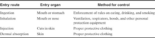
Injection, inhalation, and dermal absorption generally result in the toxicant entering the bloodstream unaltered. Toxicants entering through ingestion are frequently modified or excreted in bile.
Toxicants that enter by injection and dermal absorption are difficult to measure and quantify. Some toxicants are absorbed rapidly through the skin.
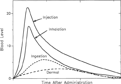
Figure 2-1 shows the expected blood-level concentration as a function of time and route of entry. The blood-level concentration is a function of a wide range of parameters, so large variations in this behavior are expected. Injection usually results in the highest blood-level concentration, followed by inhalation, ingestion, and absorption. The peak concentration generally occurs earliest with injection, followed by inhalation, ingestion, and absorption.
Figure 2-1 Toxic blood level concentration as a function of route of exposure. Wide variations are expected as a result of rate and extent of absorption, distribution, biotransformation, and excretion.
The gastrointestinal (GI) tract, the skin, and the respiratory system play significant roles in the various routes of entry.
Gastrointestinal Tract
The GI tract plays the most significant role in toxicants entering the body through ingestion. Food or drink is the usual mechanism of exposure. Airborne particles (either solid or liquid) can also lodge in the mucus of the upper respiratory tract and be swallowed.
The rate and selectivity of absorption by the GI tract are highly dependent on many conditions. The type of chemical, its molecular weight, molecule size and shape, acidity, susceptibility to attack by intestinal flora, rate of movement through the GI tract, and many other factors affect the rate of absorption.
Skin
The skin plays important roles in both the dermal absorption and injection routes of entry. Injection includes both entry by absorption through cuts and mechanical injection with hypodermic needles. Mechanical injection can occur as a result of improper hypodermic needle storage in a laboratory drawer.
The skin is composed of an outer layer called the stratum corneum. This layer consists of dead, dried cells that are resistant to permeation by toxicants. Absorption also occurs through the hair follicles and sweat glands, but this is normally negligible. The absorption properties of the skin vary as a function of location and the degree of hydration. The presence of water increases the skin hydration and results in increased permeability and absorption.
Most chemicals are not absorbed readily by the skin. A few chemicals, however, do show remarkable skin permeability. Phenol, for example, requires only a small area of skin for the body to absorb an adequate amount to result in death.
The skin on the palm of the hand is thicker than skin found elsewhere. However, this skin demonstrates increased porosity, resulting in higher toxicant absorption.
Respiratory System
The respiratory system plays a significant role in toxicants entering the body through inhalation.
The main function of the respiratory system is to exchange oxygen and carbon dioxide between the blood and the inhaled air. In 1 minute a normal person at rest uses an estimated 250 ml of oxygen and expels approximately 200 ml of carbon dioxide. Approximately 8 L of air are breathed per minute. Only a fraction of the total air within the lung is exchanged with each breath. These demands increase significantly with physical exertion.
The respiratory system is divided into two areas: the upper and the lower respiratory system. The upper respiratory system is composed of the nose, sinuses, mouth, pharynx (section between the mouth and esophagus), larynx (the voice box), and the trachea or windpipe. The lower respiratory system is composed of the lungs and its smaller structures, including the bronchi and the alveoli. The bronchial tubes carry fresh air from the trachea through a series of branching tubes to the alveoli. The alveoli are small blind air sacs where the gas exchange with the blood occurs. An estimated 300 million alveoli are found in a normal lung. These alveoli contribute a total surface area of approximately 70 m2. Small capillaries found in the walls of the alveoli transport the blood; an estimated 100 ml of blood is in the capillaries at any moment.
The upper respiratory tract is responsible for filtering, heating, and humidifying the air. Fresh air brought in through the nose is completely saturated with water and regulated to the proper temperature by the time it reaches the larynx. The mucus lining the upper respiratory tract assists in filtering.
The upper and lower respiratory tracts respond differently to the presence of toxicants. The upper respiratory tract is affected mostly by toxicants that are water soluble. These materials either react or dissolve in the mucus to form acids and bases. Toxicants in the lower respiratory tract affect the alveoli by physically blocking the transfer of gases (as with insoluble dusts) or reacting with the wall of the alveoli to produce corrosive or toxic substances. Phosgene gas, for example, reacts with the water on the alveoli wall to produce HCl and carbon monoxide.
Upper respiratory toxicants include hydrogen halides (hydrogen chloride, hydrogen bromide), oxides (nitrogen oxides, sulfur oxides, sodium oxide), and hydroxides (ammonium hydroxide, sodium dusts, and potassium hydroxides). Lower respiratory toxicants include monomers (such as acrylonitrile), halides (fluorine, chlorine, bromine), and other miscellaneous substances such as hydrogen sulfide, phosgene, methyl cyanide, acrolein, asbestos dust, silica, and soot.
Dusts and other insoluble materials present a particular difficulty to the lungs. Particles that enter the alveoli are removed slowly. For dusts the following simple rule usually applies: The smaller the dust particles, the farther they penetrate into the respiratory system. Particles greater than 5 µm in diameter are usually filtered by the upper respiratory system. Particles with diameters between 2 and 5 µm generally reach the bronchial system. Particles less than 1 µm in diameter can reach the alveoli.
2-2 How Toxicants Are Eliminated from Biological Organisms
Toxicants are eliminated or rendered inactive by the following routes:
• excretion: through the kidneys, liver, lungs, or other organs;
• detoxification: by changing the chemical into something less harmful by biotrans-formation;
• storage: in the fatty tissue.
The kidneys are the dominant means of excretion in the human body. They eliminate substances that enter the body by ingestion, inhalation, injection, and dermal absorption. The toxicants are extracted by the kidneys from the bloodstream and are excreted in the urine.
Toxicants that are ingested into the digestive tract are frequently excreted by the liver. In general, chemical compounds with molecular weights greater than about 300 are excreted by the liver into bile. Compounds with lower molecular weights enter the bloodstream and are excreted by the kidneys. The digestive tract tends to selectively detoxify certain agents, whereas substances that enter through inhalation, injection, or dermal absorption generally arrive in the bloodstream unchanged.
The lungs are also a means for elimination of substances, particularly those that are volatile. Chloroform and alcohol, for example, are excreted partially by this route.
Other routes of excretion are the skin (by means of sweat), hair, and nails. These routes are usually minor compared to the excretion processes of the kidneys, liver, and lungs.
The liver is the dominant organ in the detoxification process. The detoxification occurs by biotransformation, in which the chemical agents are transformed by reaction into either harmless or less harmful substances. Biotransformation reactions can also occur in the blood, intestinal tract wall, skin, kidneys, and other organs.
The final mechanism for elimination is storage. This process involves depositing the chemical agent mostly in the fatty areas of the organism but also in the bones, blood, liver, and kidney. Storage can create a future problem if the organism’s food supply is reduced and the fatty deposits are metabolized; the stored chemical agents will be released into the bloodstream, resulting in possible damage.
For massive exposures to chemical agents, damage can occur to the kidneys, liver, or lungs, significantly reducing the organism’s ability to excrete the substance.
2-3 Effects of Toxicants on Biological Organisms
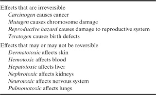
Table 2-2 lists some of the effects or responses from toxic exposure.
Table 2-2 Various Responses to Toxicants
The problem is to determine whether exposures have occurred before substantial symptoms are present. This is accomplished through a variety of medical tests. The results from these tests must be compared to a medical baseline study, performed before any exposure. Many chemical companies perform baseline studies on new employees before employment.
Respiratory problems are diagnosed using a spirometer. The patient exhales as hard and as fast as possible into the device. The spirometer measures (1) the total volume exhaled, called the forced vital capacity (FVC), with units in liters; (2) the forced expired volume measured at 1 second (FEV1), with units in liters per second; (3) forced expiratory flow in the middle range of the vital capacity (FEV 25–75%), measured in liters per second; and (4) the ratio of the observed FEV1 to FVC × 100 (FEV1/FVC%).
Reductions in expiration flow rate are indicative of bronchial disease, such as asthma or bronchitis. Reductions in FVC are due to reduction in the lung or chest volume, possibly as a result of fibrosis (an increase in the interstitial fibrous tissue in the lung). The air remaining in the lung after exhalation is called the residual volume (RV). An increase in the RV is indicative of deterioration of the alveoli, possibly because of emphysema. The RV measurement requires a specialized tracer test with helium.
Nervous system disorders are diagnosed by examining the patient’s mental status, cranial nerve function, motor system reflexes, and sensory systems. An electroencephalogram (EEG) tests higher brain and nervous system functions.
Changes in skin texture, pigmentation, vascularity, and hair and nail appearance are indicative of possible toxic exposures.
Blood counts are also used to determine toxic exposures. Measurements of the red and white blood cells, hemoglobin content, and platelet count are performed easily and inexpensively. However, blood counts are frequently insensitive to toxic exposure; marked changes are seen only after substantial exposure and damage.
Kidney function is determined through a variety of tests that measure the chemical content and quantity of urine. For early kidney damage proteins or sugars are found in the urine.
Liver function is determined through a variety of chemical tests on the blood and urine.
2-4 Toxicological Studies
A major objective of a toxicological study is to quantify the effects of the suspect toxicant on a target organism. For most toxicological studies animals are used, usually with the hope that the results can be extrapolated to humans. Once the effects of a suspect agent have been quantified, appropriate procedures are established to ensure that the agent is handled properly.
Before undertaking a toxicological study, the following items must be identified:
• the toxicant,
• the target or test organism,
• the effect or response to be monitored,
• the dose range,
• the period of the test.
The toxicant must be identified with respect to its chemical composition and its physical state. For example, benzene can exist in either liquid or vapor form. Each physical state preferentially enters the body by a different route and requires a different toxicological study.
The test organism can range from a simple single cell up through the higher animals. The selection depends on the effects considered and other factors such as the cost and availability of the test organism. For studies of genetic effects, single-cell organisms might be satisfactory. For studies determining the effects on specific organs such as the lungs, kidneys, or liver, higher organisms are a necessity.
The dose units depend on the method of delivery. For substances delivered directly into the organism (by ingestion or injection), the dose is measured in milligrams of agent per kilogram of body weight. This enables researchers to apply the results obtained from small animals such as mice (fractions of a kilogram in body weight) to humans (about 70 kg for males and 60 kg for females). For gaseous airborne substances the dose is measured in either parts per million (ppm) or milligrams of agent per cubic meter of air (mg/m3). For airborne particulates the dose is measured in milligrams of agent per cubic meter of air (mg/m3) or millions of particles per cubic foot (mppcf).
The period of the test depends on whether long- or short-term effects are of interest. Acute toxicity is the effect of a single exposure or a series of exposures close together in a short period of time. Chronic toxicity is the effect of multiple exposures occurring over a long period of time. Chronic toxicity studies are difficult to perform because of the time involved; most toxicological studies are based on acute exposures. The toxicological study can be complicated by latency, an exposure that results in a delayed response.
2-5 Dose versus Response
Biological organisms respond differently to the same dose of a toxicant. These differences are a result of age, sex, weight, diet, general health, and other factors. For example, consider the effects of an irritant vapor on human eyes. Given the same dose of vapors, some individuals will barely notice any irritation (weak or low response), whereas other individuals will be severely irritated (high response).
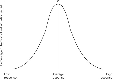
Consider a toxicological test run on a large number of individuals. Each individual is exposed to the same dose and the response is recorded. A plot of the type shown in Figure 2-2 is prepared with the data. The fraction or percentage of individuals experiencing a specific response is plotted. Curves of the form shown in Figure 2-2 are frequently represented by a normal or Gaussian distribution, given by the equation
Figure 2-2 A Gaussian or normal distributioin representing the biological response to exposure to a toxicant.
(2-1)
![]()
where
f(x) is the probability (or fraction) of individuals experiencing a specific response,
x is the response,
σ is the standard deviation, and
μ is the mean.
The standard deviation and mean characterize the shape and the location of the normal distribution curve, respectively. They are computed from the original data f(xi)using the equations
(2-2)

(2-3)
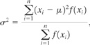
where n is the number of data points. The quantity σ2 is called the variance.
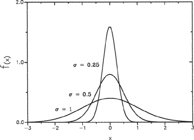
The mean determines the location of the curve with respect to the x axis, and the standard deviation determines the shape. Figure 2-3 shows the effect of the standard deviation on the shape. As the standard deviation decreases, the distribution curve becomes more pronounced around the mean value.
Figure 2-3 Effect of the standard deviation on a normal distribution with a mean of 0. The distribution becomes more pronounced around the mean as the standard deviation decreases.
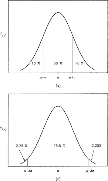
The area under the curve of Figure 2-2 represents the percentage of individuals affected for a specified response interval. In particular, the response interval within 1 standard deviation of the mean represents 68% of the individuals, as shown in Figure 2-4a. A response interval of 2 standard deviations represents 95.5% of the total individuals (Figure 2-4b). The area under the entire curve represents 100% of the individuals.
Figure 2-4 Percentage of individuals affected based on a response between one and two standard deviations of the mean.
Example 2-1
Seventy-five people are tested for skin irritation because of a specific dose of a substance. The responses are recorded on a scale from 0 to 10, with 0 indicating no response and 10 indicating a high response. The number of individuals exhibiting a specific response is given in the following table:

a. Plot a histogram of the number of individuals affected versus the response.
b. Determine the mean and the standard deviation.
c. Plot the normal distribution on the histogram of the original data.
Solution.
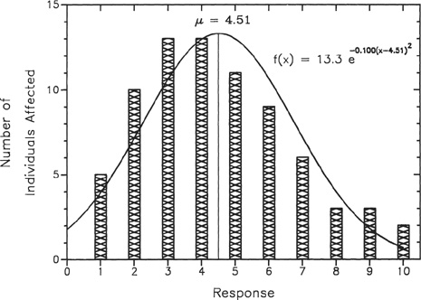
The histogram is shown in Figure 2-5. The number of individuals affected is plotted versus the response. An alternative method is to plot the percentage of individuals versus the response.
Figure 2-5 Percentage of individuals affected based on response.
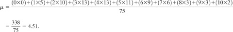
b. The mean is computed using Equation 2-2 :
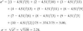
The standard deviation is computed using Equation 2-3:
c. The normal distribution is computed using Equation 2-1. Substituting the mean and standard deviations, we find
![]()
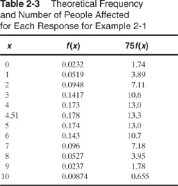
The distribution is converted to a function representing the number of individuals affected by multiplying by the total number of individuals, in this case 75. The corresponding values are shown in Table 2-3 and Figure 2-5.
Table 2-3 Theoretical Frequency and Number of People Affected for Each Response for Example 2-1
The toxicological experiment is repeated for a number of different doses, and normal curves similar to Figure 2-3 are drawn. The standard deviation and mean response are determined from the data for each dose.
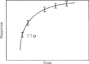
A complete dose-response curve is produced by plotting the cumulative mean response at each dose. Error bars are drawn at ±σ around the mean. A typical result is shown in Figure 2-6.
Figure 2-6 Dose-response curve. The bars around the data points represent the standard deviation in response to a specific dose.
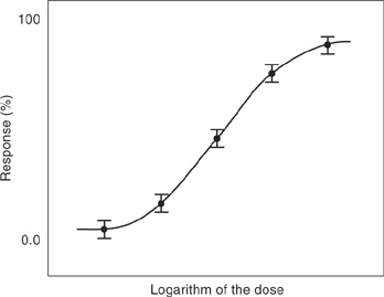
For convenience, the response is plotted versus the logarithm of the dose, as shown in Figure 2-7. This form provides a much straighter line in the middle of the response curve than the simple response versus dose form of Figure 2-6.
If the response of interest is death or lethality, the response versus log dose curve of Figure 2-7 is called a lethal dose curve. For comparison purposes the dose that results in 50%
Figure 2-7 Response versus log dose curve. This form presents a much straighter function than the one shown in Figure 2-6.
lethality of the subjects is frequently reported. This is called the LD50 dose (lethal dose for 50% of the subjects). Other values such as LD10 or LD90 are sometimes also reported. For gases, LC (lethal concentration) data are used.
If the response to the chemical or agent is minor and reversible (such as minor eye irritation), the response–log dose curve is called the effective dose (ED) curve. Values for ED50,ED10, and so forth are also used.
Finally, if the response to the agent is toxic (an undesirable response that is not lethal but is irreversible, such as liver or lung damage), the response–log dose curve is called the toxic dose, or TD curve.
The relationship between the various types of response–log dose curves is shown in Figure 2-8.
Figure 2-8 The various types of response vs. log dose curves. ED, effective dose; TD, toxic dose; LD, lethal dose. For gases, LC (lethal concentration) is used.

Most often, response-dose curves are developed using acute toxicity data. Chronic toxicity data are usually considerably different. Furthermore, the data are complicated by differences in group age, sex, and method of delivery. If several chemicals are involved, the toxicants might interact additively (the combined effect is the sum of the individual effects), synergistically (the combined effect is more than the individual effects), potentiately (presence of one increases the effect of the other), or antagonistically (both counteract each other).
2-6 Models for Dose and Response Curves
Response versus dose curves can be drawn for a wide variety of exposures, including exposure to heat, pressure, radiation, impact, and sound. For computational purposes the response versus dose curve is not convenient; an analytical equation is preferred.
Many methods exist for representing the response-dose curve.1 For single exposures the probit (probit= probability unit) method is particularly suited, providing a straight—line equivalent to the response-dose curve. The probit variable Y is related to the probability P by2
1Phillip L. Williams and James L. Burson, eds., Industrial Toxicology: Safety and Health Applications in the Workplace (New York: Van Nostrand Reinhold, 1985), p. 379.
2D. J. Finney, Probit Analysis (Cambridge: Cambridge University Press, 1971), p. 23.
(2-4)
![]()
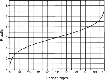
Equation 2-4 provides a relationship between the probability P and the probit variable Y. This relationship is plotted in Figure 2-9 and tabulated in Table 2-4.
Figure 2-9 The relationship between percentages and probits. (Source: D. J. Finney, Probit Analysis, 3d ed. (Cambridge: Cambridge University Press, 1971), p. 23. Reprinted by permission.
The probit relationship of Equation 2-4 transforms the sigmoid shape of the normal response versus dose curve into a straight line when plotted using a linear probit scale, as shown in Figure 2-10. Standard curve-fitting techniques are used to determine the best-fitting straight line.
Figure 2-10 The probit transformation converts the sigmoidal response vs. log dose curve into a straight line when plotted on a linear probit scale. Source: D. J. Finney, Probit Analysis, 3d ed. (Cambridge: Cambridge University Press, 1971), p. 24. Reprinted by permission.
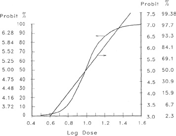
Table 2-5 lists a variety of probit equations for a number of different types of exposures. The causative factor represents the dose V. The probit variable Y is computed from
(2-5)
![]()
Table 2-4 Transformation from Percentages to Probits1
1D. J. Finney, Probit Analysis, (Cambridge: Cambridge University Press, 1971), p. 25. Reprinted by permission.
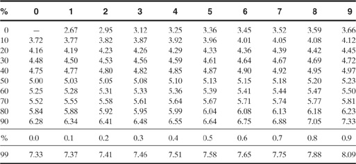
Table 2-5 Probit Correlations for a Variety of Exposures (The causative variable is representative of the magnitude of the exposure.)
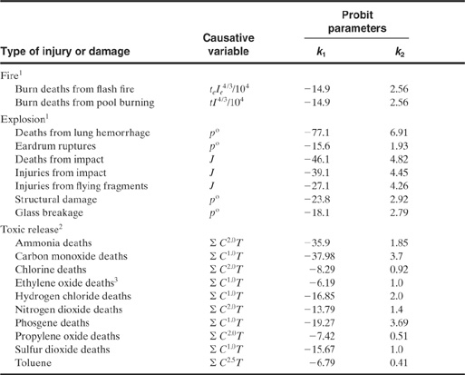
te = effective time duration (s)
Ie = effective radiation intensity (W/m2)
t = time duration of pool burning (s)
I = radiation intensity from pool burning (W/m2)
po = peak overpressure (N/m2)
J = impulse (N s/m2)
C = concentration (ppm)
T = time interval (min)
1Selected from Frank P. Lees, Loss Prevention in the Process Industries (London: Butterworths, 1986), p. 208.
2CCPS, Guidelines for Consequence Analysis of Chemical Releases (New York: American Institute of Chemical Engineers, 1999), p. 254.
3Richard W. Purgh, “Quantitative Evaluation of Inhalation Toxicity Hazards,” in Proceedings of the 29th Loss Prevention Symposium (American Institute of Chemical Engineers, July 31, 1995).
For spreadsheet computations a more useful expression for performing the conversion from probits to percentage is given by
(2-6)
![]()
where erf is the error function.
Example 2-2
Determine the percentage of people who will die as a result of burns from pool burning if the probit variable Y is 4.39. Compare results from Table 2-4 and Equation 2-6.
Solution
The percentage from Table 2-4 is 27%. The same percentage can be computed using Equation 2-6, as follows:
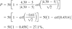
where the error function is a mathematical function found in spreadsheets, Mathcad, and other software programs.
Example 2.3
Eisenberg3 reported the following data on the effect of explosion peak overpressures on eardrum rupture in humans:
3N. A. Eisenberg, Vulnerability Model: A Simulation System for Assessing Damage Resulting from Marine Spills, NTIS Report AD-A015-245 (Springfield, VA: National Technical Information Service, 1975).
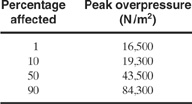
Confirm the probit correlation for this type of exposure, as shown in Table 2-5.
Solution
The percentage is converted to a probit variable using Table 2-4. The results are:
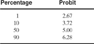
Figure 2-11 Percentage affected versus the natural logarithm of the peak overpressure for Example 2-3.
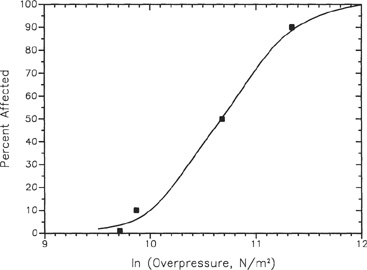
Figure 2-11 is a plot of the percentage affected versus the natural logarithm of the peak overpressure. This demonstrates the classical sigmoid shape of the response versus log dose curve. Figure 2-12 is a plot of the probit variable (with a linear probit scale) versus the natural logarithm of the peak overpressure. The straight line verifies the values reported in Table 2-5. The sigmoid curve of Figure 2-11 is drawn after converting the probit correlation back to percentages.
Figure 2-12 Probit versus the natural logarithm of the peak overpressure for Example 2-3.
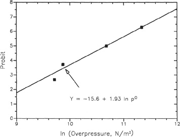
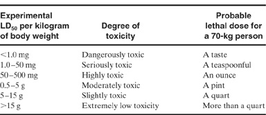
Table 2-6 Hodge-Sterner Table for Degree of Toxicity1
1N. Irving Sax, Dangerous Properties of Industrial Materials (New York: Van Nostrand Reinhold, 1984), p. 1.
2-7 Relative Toxicity
Table 2-6 shows the Hodge-Sterner table for the degree of toxicity. This table covers a range of doses from 1.0 mg/kg to 15,000 mg/kg.
Toxicants are compared for relative toxicity based on the LD, ED, or TD curves. If the response-dose curve for chemical A is to the right of the response-dose curve for chemical B, then chemical A is more toxic. Care must be taken when comparing two response-dose curves when partial data are available. If the slopes of the curves differ substantially, the situation shown in Figure 2-13 might occur. If only a single data point is available in the upper part of the curves, it might appear that chemical A is always more toxic than chemical B. The complete data show that chemical B is more toxic at lower doses.
2-8 Threshold Limit Values
The lowest value on the response versus dose curve is called the threshold dose. Below this dose the body is able to detoxify and eliminate the agent without any detectable effects. In reality the response is only identically zero when the dose is zero, but for small doses the response is not detectable.
The American Conference of Governmental Industrial Hygienists (ACGIH) has established threshold doses, called threshold limit values (TLVs), for a large number of chemical agents. The TLV refers to airborne concentrations that correspond to conditions under which no adverse effects are normally expected during a worker’s lifetime. The exposure occurs only during normal working hours, eight hours per day and five days per week. The TLV was formerly called the maximum allowable concentration (MAC).
There are three different types of TLVs (TLV-TWA, TLV-STEL, and TLV-C) with precise definitions provided in Table 2-7. More TLV-TWA data are available than TWA-STEL or TLV-C data.
OSHA has defined its own threshold dose, called a permissible exposure level (PEL).
Figure 2-13 Two toxicants with differing relative toxicities at different doses. Toxicant A is more toxic at high doses, whereas toxicant B is more toxic at low doses.

Table 2-7 Definitions for Threshold Limit Values (TLVs)1
1TLVs should not be used for (1) a relative index of toxicity, (2) air pollution work, or (3) assessment of toxic hazard from continuous, uninterrupted exposure.

PEL values follow the TLV-TWA of the ACGIH closely. However, the PEL values are not as numerous and are not updated as frequently. TLVs are often somewhat more conservative.
For some toxicants (particularly carcinogens) exposures at any level are not permitted. These toxicants have zero thresholds.
Another quantity frequently reported is the amount immediately dangerous to life and health (IDLH). Exposures to this quantity and above should be avoided under any circumstances.
TLVs are reported using ppm (parts per million by volume), mg/m3 (milligrams of vapor per cubic meter of air), or, for dusts, mg/m3 or mppcf (millions of particles per cubic foot of air). For vapors, mg/m3 is converted to ppm using the equation
(2-7)
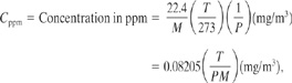
where
T is the temperature in degrees Kelvin,
P is the absolute pressure in atm, and
M is the molecular weight in g/g-mol.
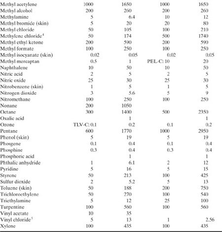
TLV and PEL values for a variety of toxicants are provided in Table 2-8.
Table 2-8 TLVs and PELs for a Variety of Chemical Substances
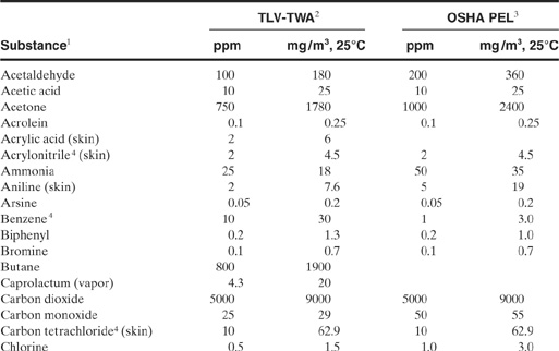

1Latest NIOSH Pocket Guide information is available at the NIOSH web site: http://www.cdc.gov/noish.
2Documentation of the Threshold Limit Values and Biological Exposure Indices, 5th ed. (Cincinnati: American Conference of Governmental Industrial Hygienists, 1991-1994).
3NIOSH Pocket Guide to Chemical Hazards (Cincinnati: National Institute for Occupational Safety and Health, 2000).
4Possible carcinogen.
5Human carcinogen.
The ACGIH clearly points out that the TLVs should not be used as a relative index of toxicity (see Figure 2-8), should not be used for air pollution work, and cannot be used to assess the impact of continuous exposures to toxicants. The TLV assumes that workers are exposed only during a normal eight-hour workday.
Every effort must be made to reduce worker exposures to toxicants to below the PEL and lower if possible.
Suggested Reading
Toxicology
Howard H. Fawcett and William S. Wood, eds., Safety and Accident Prevention in Chemical Operations, 2d ed. (New York: Wiley, 1982), ch. 14, 15, and 25.
N. Irving Sax, Dangerous Properties of Industrial Materials, 6th ed. (New York: Van Nostrand Reinhold, 1984), sec. 1.
Phillip L. Williams and James L. Burson, eds., Industrial Toxicology: Safety and Health Applications in the Workplace (New York: Van Nostrand Reinhold, 1985).
Probit Analysis
D. J. Finney, Probit Analysis (Cambridge: Cambridge University Press, 1971).
Frank P. Lees, Loss Prevention in the Process Industries (London: Butterworths, 1986), p. 207.
Frank P. Lees, Loss Prevention in the Process Industries, 2d ed. (London: Butterworths, 1996).
Threshold Limit Values
Documentation of the Threshold Limit Values and Biological Exposure Indices, 5th ed. (Cincinnati: American Conference of Governmental Industrial Hygienists, 1986).
Health Effects Assessment Summary Tables (HEASH), OERR 9200.6-303 (Cincinnati: Center for Environmental Research Information, 1991).
Integrated Risk Information System (IRIS) (Cincinnati: Center for Environmental Research Information, updated regularly).
Problems
2-1. Derive Equation 2-7.
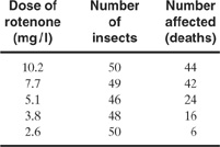
2-2. Finney4 reported the data of Martin5 involving the toxicity of rotenone to the insect species Macrosiphoniella sanborni. The rotenone was applied in a medium of 0.5% saponin, containing 5% alcohol. The insects were examined and classified one day after spraying. The obtained data were:
4D. J. Finney, Probit Analysis (Cambridge: Cambridge University Press, 1971), p. 20.
5J. T. Martin, “The Problem of the Evaluation of Rotenone-Containing Plants. VI. The Toxicity of l-Elliptone and of Poisons Applied Jointly, with Further Observations on the Rotenone Equivalent Method of Assessing the Toxicity of Derris Root,” Ann. Appl. Biol. (1942), 29: 69–81.
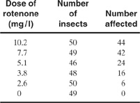
a. From the given data, plot the percentage of insects affected versus the natural logarithm of the dose.
b. Convert the data to a probit variable, and plot the probit versus the natural logarithm of the dose. If the result is linear, determine a straight line that fits the data. Compare the probit and number of insects affected predicted by the straight-line fit to the actual data.
2-3. A blast produces a peak overpressure of 47,000 N/m2. What fraction of structures will be damaged by exposure to this overpressure? What fraction of people exposed will die as a result of lung hemorrhage? What fraction will have eardrums ruptured? What conclusions about the effects of this blast can be drawn?
2-4. The peak overpressure expected as a result of the explosion of a tank in a plant facility is approximated by the equation
log P = 4.2 − 1.8 log r,
where P is the overpressure in psi and r is the distance from the blast in feet. The plant employs 500 people who work in an area from 10 to 500 ft from the potential blast site. Estimate the number of fatalities expected as a result of lung hemorrhage and the number of eardrums ruptured as a result of this blast. Be sure to state any additional assumptions.
2-5. A certain volatile substance evaporates from an open container into a room of volume 1000 ft3. The evaporation rate is determined to be 100 mg/min. If the air in the room is assumed to be well mixed, how many ft3/min of fresh air must be supplied to ensure that the concentration of the volatile is maintained below its TLV of 100 ppm? The temperature is 77°F and the pressure is 1 atm. Assume a volatile species molecular weight of 100. Under most circumstances the air in a room cannot be assumed to be well mixed. How would poor mixing affect the quantity of air required?
2-6. In Example 2-1, part c, the data were represented by the normal distribution function
f(x) = 0.178e-0.100(x-4.51)2.
Use this distribution function to determine the fraction of individuals demonstrating a response between the range of 2.5 to 7.5.
2-7. How much acetone liquid (in milliliters) is required to produce a vapor concentration of 200 ppm in a room of dimension 3 × 4 × 10 m? The temperature is 25°C and the pressure is 1 atm. The following physical property data are for acetone: molecular weight, 58.1; and specific gravity, 0.7899.
2-8. If 500 workers in a plant are exposed to the following concentrations of ammonia for the given number of hours, how many deaths will be expected?
a. 1000 ppm for 1 hour.
b. 2000 ppm for 2 hours.
c. 300 ppm for 3 hours.
d. 150 ppm for 2 hours.
2-9. Use the NIOSH web site (www.cdc.gov/niosh) to acquire the meaning and definition of IDLH concentration.
2-10. Use the NIOSH web site to determine an escape time period for a person subjected to an IDLH concentration.
2-11. Use the NIOSH web site to determine the number of deaths that occurred in 1992 as a result of asbestos.
2-12. Use the NIOSH web site to determine and compare the PEL and the IDLH concentration of ethylene oxide and ethanol.
2-13. Use the NIOSH web site to determine and compare the PEL, IDLH concentration, and TLV for ethylene oxide, benzene, ethanol, ethylene trichloride, fluorine, and hydrogen chloride.
2-14. Use the NIOSH web site to determine and compare the PEL, IDLH concentration, and LC50 for ammonia, carbon monoxide, and ethylene oxide.
2-15. The NIOSH web site states that deaths occur as a result of ammonia exposures between 5,000 and 10,000 ppm over a 30-min period. Compare the result to the results from the probit equation (Table 2-5).
2-16. Use the probit equation (Equation 2-5) to determine the expected fatalities for people exposed for 2 hours to each of the IDLH concentrations of ammonia, chlorine, ethylene oxide, and hydrogen chloride.
2-17. Determine the concentration of ethylene oxide that will cause a 50% fatality rate if the exposure occurs for 30 min.
2-18. A group of 100 people is exposed to phosgene in two consecutive periods as follows: (a) 10 ppm for 30 min and (b) 1 ppm for 300 min. Determine the expected number of fatalities.
2-19. Determine the duration times, in minutes, that a group of 100 people can be exposed to 1500 ppm of carbon monoxide to result in (a) 0% fatalities and (b) 50% fatalities.
2-20. Use Equation 2-7 to convert the TLV in ppm to the TLV in mg/m3 for benzene, carbon monoxide, and chlorine. Assume 25°C and 1 atm.
2-21. Use a spreadsheet program (such as QuattroPro, Lotus, Excel) to solve Problem 2-4. Break the distance from 10 ft to 500 ft into several intervals. Use a small enough distance increment so that the results are essentially independent of the increment size. Your spreadsheet output should have designated columns for the distance, pressure, probit values, percentages, and the number of individuals affected for each increment. You should also have two spreadsheet cells that provide the total number of individuals with eardrum ruptures and lung hemorrhage deaths. For converting from probits to percentages, use a lookup function or an equivalent function.
2-22. Use the results of Problem 2-21 to establish the recommended distance between the control room and the tank if the control room is designed to withstand overpressures of (a) 1 psi and (b) 3 psi.
2-23. Use Equation 2-6 to convert probits of 3.72, 5.0, and 6.28 to percentage affected, and compare with the values shown in Table 2-4.
2-24. Estimate the exposure concentration in ppm that will result in fatalities for 80% of the exposed individuals if they are exposed to phosgene for 4 min.
2-25. Estimate the exposure concentration in ppm that will result in fatalities for 80% of the exposed individuals if they are exposed to chlorine for 4 min.
2-26. Determine the potential deaths resulting from the following exposure to chlorine:
a. 200 ppm for 15 min.
b. 100 ppm for 5 min.
c. 50 ppm for 2 min.
2-27. Determine the potential deaths resulting from the following exposure to chlorine:
a. 200 ppm for 150 min.
b. 100 ppm for 50 min.
c. 50 ppm for 20 min.
2-28. Use Joseph F. Louvar and B. Diane Louvar, Health and Environmental Risk Analysis: Fundamentals with Applications (Upper Saddle River, NJ: Prentice Hall, 1998), pp. 287–288, to find the toxicity levels (high, medium, low) for the inhalation of toxic chemicals.
2-29. Use Louvar and Louvar, Health and Environmental Risk Analysis, pp. 287–288, to find the toxicity levels (high, medium, low) for the single dose of a chemical that causes 50% deaths.
2-30. Using the following data, determine the probit constants and the LC50: