Now that we have discussed the chicken, let’s discuss the egg. In earlier chapters, configuration examples and details about several control plane protocols were provided. This chapter discusses what it means to be a control plane protocol, how these protocols interact, and how to secure the control plane and provides additional configuration examples.
The control plane makes the decisions that the data plane uses when forwarding data. Typically, when one thinks about the control plane, routing protocols and the spanning tree come to mind. There are also control plane protocols that support other control plane functions. Two examples are Domain Name System (DNS) and Network Time Protocol (NTP). DNS provides name resolution, which is required to map names to logical addresses prior to making decisions on those addresses. NTP provides time synchronization, which is required by protocols that require time, such as time-based access control lists (ACLs) or authentication key chains.
Our discussion starts with the control plane at layer 2 and then moves up the protocol stack to the layer 3 control plane protocols. Due to the way protocols are intertwined, we will overlap with sections on routing and switching.
Layer 2
Even at layer 2, the data plane and control plane are interdependent. The control plane can’t function without the data plane, and the functionality of the data plane is limited to an inefficient local scope without the assistance of the control plane.
Ethernet loop prevention was discussed in Chapter 5. One technique for loop prevention is to physically design the network so loops aren’t possible. The more common technique is to use the Spanning Tree Protocol (STP ). The Ethernet will function without it, but at a risk of completely saturating the links with broadcast storms. To recap slightly, STP elects a root bridge, and then all other switches calculate the best path to the root bridge and block alternative paths. Per-VLAN Spanning Tree (PVST) helps minimize waste of bandwidth by calculating a tree for each VLAN. This allows for a different root and different paths for each VLAN. However, the resources required for PVST increase with each additional VLAN.
PVST is Cisco proprietary. With that said, you can connect a Cisco switch that is part of a PVST domain with another vendor’s switch running MST. They will just use an interoperability mode to connect the trees. In addition to the improved resource utilization of MST over PVST, design limitations of the original Spanning Tree Protocol were addressed. MST includes features to detect changes much faster than the original STP. These changes are also present in Cisco’s Rapid Per-VLAN Spanning Tree. Switches with IOS-XE code greater than 16.x default to Rapid-PVST, even though we often still refer to it as PVST. Switches with earlier versions of code default to legacy PVST and should be changed to either MST or Rapid-PVST using the command spanning-tree mode {mst|rapid-pvst}.
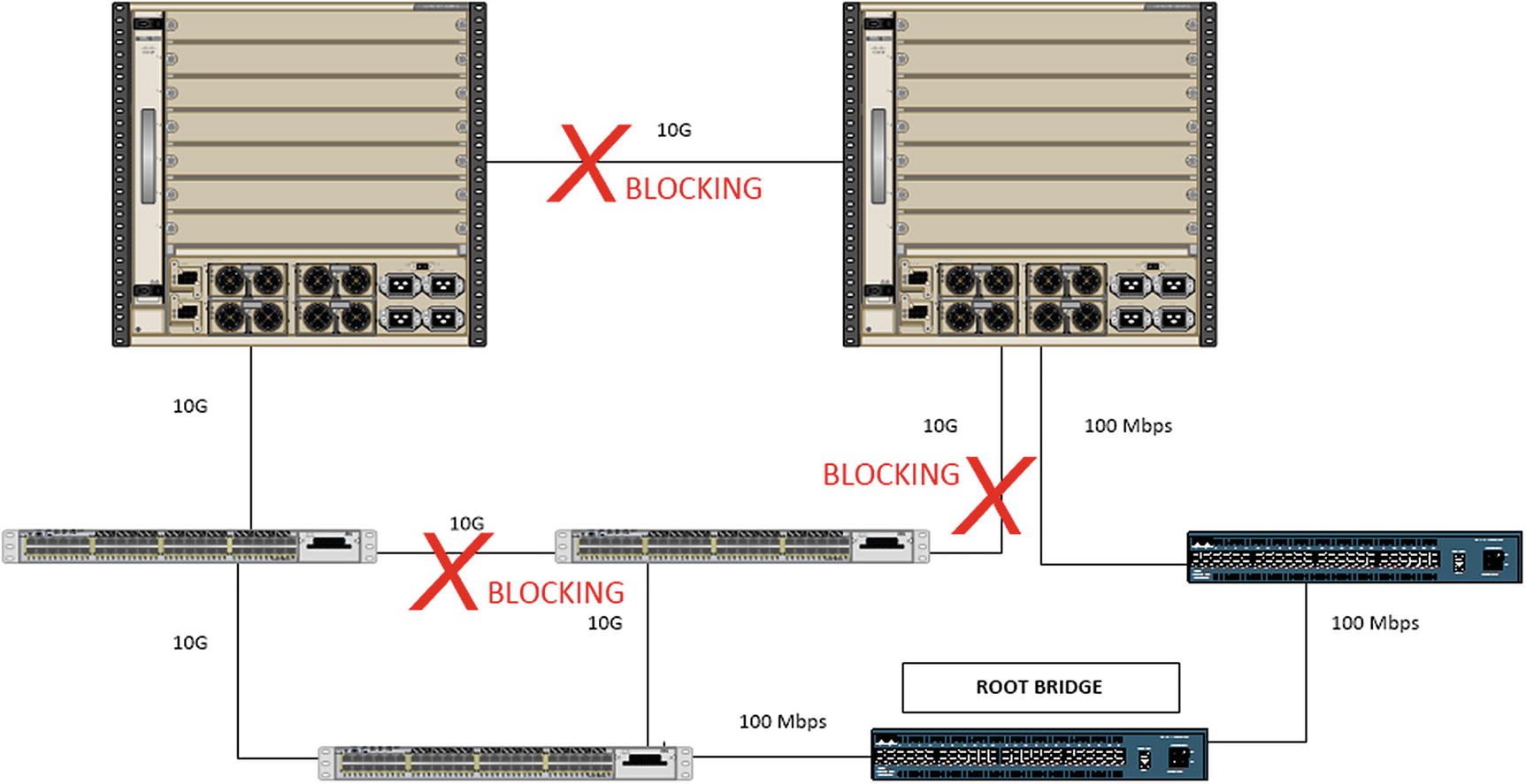
A bad switch design with a bad root bridge
In most cases, the default root bridge election results in a suboptimal choice of root bridges. To improve the tree, the bridge priority should be configured on switches that should win the election. The bridge with the lowest priority wins. To further improve the tree and eliminate the risk of nonoptimal or unknown devices taking the root role, layer 2 protocols such as BPDU Guard and Root Guard can be used.
Layer 2 and 3 Interaction
Layer 2 loop prevention is important, but even with a non-looped layer 2 network, data cannot route to other networks without help from the control plane. The Address Resolution Protocol (ARP) is the glue between layer 2 and layer 3 for IPv4. Without ARP, you can’t really even statically route traffic, because you need ARP or static mapping to find the layer 2 address of the layer 3 next hop. Dynamic routing protocols depend on ARP just as much as static routing. The resulting Routing Information Base from dynamic protocols still needs ARP to determine the layer 2 addresses of the next hops, and you have the extra step of discovering neighbors and forming relationships. As we move to IPv6, ICMP neighbor discovery takes its place, but the concept is roughly the same.
Routing Protocols
Routing protocols were discussed in Chapter 6. These are all examples of control plane protocols. This chapter further discusses securing these protocols with access lists and authentication and also discusses a few more aspects about how the protocols function and interact. We will hit routing protocols once again in Chapter 14 where we discuss advanced topics.
Interior Gateway Protocols
Interior Gateway Protocols get their name because they are used between routers on the interior of a network. They operate within an autonomous system (AS ). The interior protocols have limited scalability, and in most cases, they can react quickly to network changes.
The manner in which they react to network changes can actually cause problems for large networks. For example, when a network change is detected by Open Shortest Path First (OSPF), it causes a recalculation on all of the routers in the area. This is a reason to keep areas small.
Even with the more efficient incremental calculation, you want to minimize how many LSAs are flooded. To recap from Chapter 6, Area Border Routers (ABRs) summarize the router and network LSAs into summary LSAs. The summaries reduce the effect of flapping links.
To further reduce the effect of topology changes, you can look at different area types. For example, a totally stubby area is used when there is only one way out of an area. In this case, the topology outside of the area isn’t relevant, and the ABR only needs to advertise a default route.

Area Border Routers
There is a way to work around this scalability issue in OSPF’s control plane; this is with virtual links. A virtual link creates a control plane tunnel that is part of Area 0. This special tunnel only allows OSPF control plane traffic and no data plane traffic. A virtual link is configured by specifying the area over which it will tunnel and the router ID of the peer ABR. These tunnels can even be configured in serial to hop over several areas, but if your design includes a series of areas that are not attached to Area 0, you should rethink your design. Virtual links are usually employed as Band-Aid fixes for merging topologies and are usually dispensed with when an outage can be incurred and the topology reconfigured.
Another way to reach the backbone area from a remote area is to use a data plane tunnel. Using this option, you don’t need transit areas, so you can make better use of summarization, but this can also lead to suboptimal routing. Tunneling and the interarea route selection process are discussed in Chapter 15.
The Enhanced Interior Gateway Routing Protocol (EIGRP ) has a different set of control plane advantages and disadvantages than OSPF. One disadvantage of EIGRP is that it was a Cisco proprietary protocol. It was opened by Cisco in 2013, so it hasn’t been fully adopted by other vendors yet. However, that isn’t a control plane issue.
EIGRP is an advanced distance-vector protocol. Chapter 6 mentions that it uses the Diffusing Update Algorithm (DUAL), but that chapter focuses more on implementation than control plane mechanisms. DUAL uses the concept of feasible distance and reported distance to determine optimal routes. The reported distance is the distance reported by a peer to get to a network. The feasible distance is the distance reported by the peer, including the distance to that peer. A route is a successor, which means it is eligible to be put in the routing table, if the reported distance is less than the feasible distance. Sounds confusing, right? When you look at the logic behind it, it is easy to understand. To use a physical example, you can get to Honolulu from Ewa Beach in 21.4 miles if your first turn is onto the H-1. So 21.4 miles would be your feasible distance. Someone tells you that they know a path that is 24 miles from where they are located. This is the reported distance. Not knowing anything other than distance, you can’t guarantee that they aren’t having you do a 2.6-mile loop and then come right back to your starting place. It isn’t necessarily a loop, but you can’t take the chance. On the other hand, if someone tells you that they know a path from their location that is 19 miles, there isn’t any way that they are going through the current location to get there.
In the previous example, you used miles as a distance. A better comparison to the distance used by EIGRP is to include speed limit and congestion. In many cases, it is actually physically further to take the highway than to take side roads, but you go faster on the highway. The same applies to networking. You don’t want to hop through legacy serial links or satellites when you can use an optical transport. With that in mind, the following is the legacy equation for calculating an EIGRP’s distance metric:
metric = ([K1 * scaled minimum bandwidth + (K2 * scaled minimum bandwidth ) / (256 – load) + K3 * scaled delay] * [K5 / (reliability + K4)]) * 256
The K values correspond to binary settings configured on the EIGRP process. The default is K1 = 1 and K3 = 1, and the rest are 0. When K5 = 0, that portion of the equation is ignored, rather than multiplying by 0. This simplifies the default distance metric calculation to the following:
Take another look at the preceding output from show ip protocols. There are some differences from the output you saw in Chapter 6. This is due to configuring EIGRP using named mode instead of autonomous system mode. In the case of EIGRP, using the different configuration methods makes minor changes to the protocol. The main changes are the introduction of a wide metric and a K6 value. The values for delay and bandwidth in the previously shown equation are actually scaled. The problem with the legacy scaling is that any interface above 1 Gbps will have the same scaled bandwidth. The 64-bit-wide metric improves this limitation by changing the scale by a factor of 65536. This raises the point where links become equal to 4.2 terabits. One issue is that unless all routers in the autonomous system are configured to use the wide metric, they will revert to the legacy metric. A word of caution when you get to redistribution: Many example documents use redistribution metrics of “1 1 1 1 1”. This does not work with wide metrics.
The external administrative distance and EIGRP router IDs are both used for loop prevention during redistribution. The default administrative distance of EIGRP is 90, but when the route is external, it has a default administrative distance of 170. This means that an internal route will always be considered before the external route and will mitigate issues from arbitrary metrics set during redistribution. With EIGRP, the router ID is primarily used with redistributed routes. When a router tries to redistribute a route that has its router ID, it will discard it as a loop. Assuming there aren’t duplicate router IDs, it would be correct in this assumption. In older versions of IOS, the router ID was only checked during redistribution. Starting in 15.x, the router ID was also checked with internal EIGRP.
Last, and in this case least, let’s discuss some control plane aspects of RIP. RIP is rarely used in live networks anymore, and with an administrative distance of 120, it loses to internal EIGRP and OSPF. When dynamic routing was young and routers didn’t have many resources, RIP’s simplicity provided its value. Even in modern networks, where all links are equal, it can be a viable protocol. When the link speeds are not equal, RIP quickly loses value. The simple hop count metric used by RIP is similar to using a count of the number of roads to get to a destination. By RIP’s logic, it is better to take H-1 to Highway 72 to get to Waimanalo from Aiea, because of the road count of two. However, if you take average speed into account, the better route is H-201 to H-3 to Highway 83 to Highway 72, which is a road count of four.
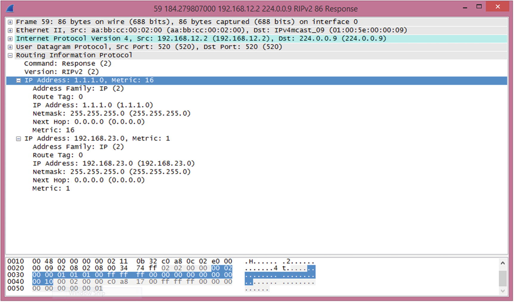
RIP route poisoning
The routing control plane isn’t just about exchanging routes. It also includes security for those route exchanges. Most of the protocols have built-in security controls such as TTL checks and authentication. In addition to those built-in mechanisms, you can also use access lists to protect the control plane.
For example, OSPF packets should typically only be transmitted on a local segment. If there is a concern that an intruder may try to inject information into OSPF, you can check TTL. For protocols that only need a TTL of 1, and they are normally sent with a TTL of 1, an intruder can craft a packet so it has a TTL of 1 by the time it arrives. If you change the rule and say that you expect a packet to arrive with a TTL of 254, it is more difficult for an intruder to inject a packet. This is because the maximum TTL is 255 and the value would be decremented if it passed through any routers.
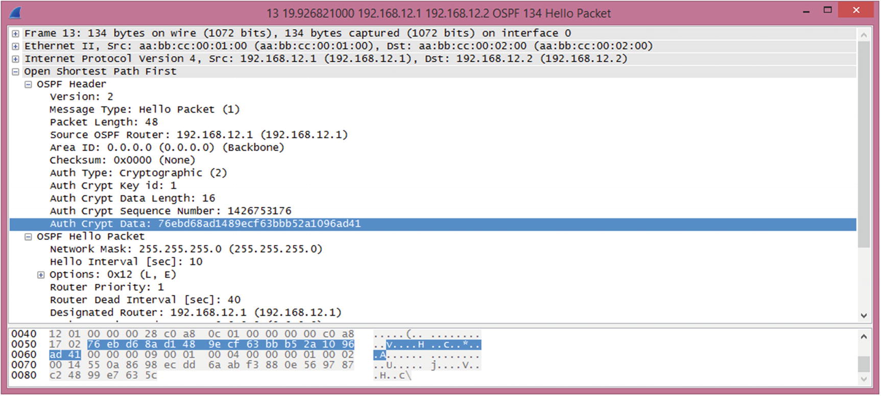
OSPF MD5 authentication
OSPF authentication is enabled on the area. Virtual links are part of Area 0 and must use Area 0’s authentication. This is often forgotten, and due to the on-demand nature of virtual links, the problem likely won’t present itself immediately.
The configuration of OSPFv3 is close to OSPFv2, but it has a few improvements. OSPFv3 does not need to use TTL security because it uses IPv6 link-local addresses for its transport. Link-local addresses only have a local scope. TTL security is only available for virtual links and sham links. It improves authentication using stronger encryption. Instead of using a simple hash, it can either encrypt the entire payload or authenticate the packet using AES or DES.
In modern versions of IOS and IOS-XE, both named mode and classic mode EIGRP are available. This causes some complications with EIGRP authentication. An issue that many engineers encounter with this version is that it allows you to enter classic mode authentication commands, even when the EIGRP process was created in named mode, but it will not apply to the EIGRP process. With named mode EIGRP, all configuration is done under the router EIGRP process.
At this point, you aren’t done. The EIGRP configuration references a key chain. The string at the end of the command is the name of the key chain and not the key itself. This makes it easier to rotate keys. Using a key chain, you can configure keys to have overlapping lifetimes, which reduces the risk of a router sending a key that the other router doesn’t accept.
This is also a good way to recover type 7 encrypted passwords found elsewhere in a configuration. This only works with type 7 encryption, not the stronger type 5 that uses an MD5 hash. Type 7 encryption is the protection obtained when service password-encryption is enabled. If you are using AES to encrypt pre-shared keys, this technique will not work.
Named mode EIGRP applies everything to the EIGRP process. All interface-specific configuration is applied to the af-interface under the EIGRP address family. Default configurations for all interfaces are under af-interface default.
In this example, all the traffic you want to go to the router is allowed, and everything else is denied. Specifically, you allowed EIGRP traffic from 192.168.12.2, ICMP traffic from anywhere, and SSH from 10.1.1.0/24. For traffic destined to 192.168.12.1 on the router, traffic that wasn’t previously allowed is blocked by the explicit deny statement. All other traffic going through the router is then explicitly allowed. It is extremely important to include the permit statement at the end. Otherwise, the implicit deny at the end of access lists would prevent the flow of transit traffic.
When writing this type of access list, make sure that you know all the traffic that should be allowed. A tool to help determine if you missed traffic is to temporarily log hits on the deny list. Once you are confident that you are allowing everything you need, remove the log parameter to reduce the performance impact of the access list.
Exterior Gateway Protocols
The Border Gateway Protocol (BGP ) is the exterior gateway protocol of the Internet. It is comprised of an interior component, iBGP, and an exterior component, eBGP.
It is arguable that iBGP is actually an interior protocol and not just the portion of an exterior protocol that communicates within an autonomous system. If you use the definition that an IGP is a protocol for exchanging prefixes within an autonomous system, then it meets the definition when synchronization is disabled. A router with synchronization enabled will not install a route learned through iBGP unless it can validate the route through an IGP. Just stating this implies that iBGP is not an IGP. However, with synchronization disabled, iBGP can be used as the only routing protocol within an autonomous system.
Even when using iBGP as the only routing protocol within the autonomous system, it has some control plane concerns that aren’t present in IGPs. BGP will not advertise prefixes learned through iBGP to another iBGP peer. To ensure that all the iBGP speakers have identical tables, there must either be a full mesh peering all of the speakers in the autonomous system, or a method such as confederations or route reflectors must be used. A full mesh requires n*(n – 1)/2 relationships. In the case of four iBGP speakers, that is six relationships. In this case, you wouldn’t need to reduce the number of peers. How about if you have ten iBGP speakers? You are already up to 45 peers, and it continues to grow quickly.
A BGP confederation essentially breaks an autonomous system into sets of smaller autonomous systems. This reduces the number of peering relationships because the routers connecting the confederation peers behave similarly to eBGP.
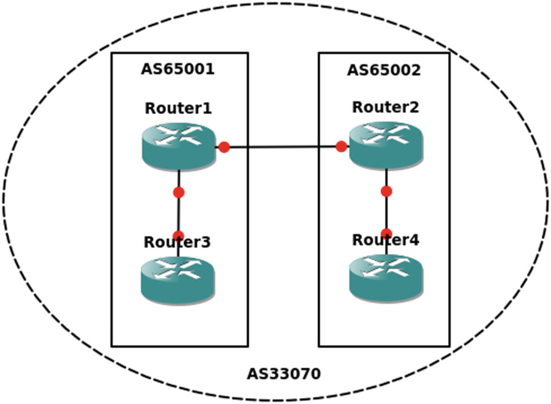
iBGP confederation
Route reflectors use a slightly different approach. In many ways, it is even simpler to configure a route reflector than a confederation. A route reflector still acts like an iBGP peer, except that it reflects iBGP routes to its clients. To configure a router as a reflector, simply add a neighbor statement with the token route-reflector-client.
A prefix learned from an eBGP peer is passed to both clients and non-clients.
A prefix learned from a client will be passed to both clients and non-clients.
A prefix learned from non-clients will be passed only to clients.
It is best practice to put the route reflectors at the edge of the autonomous system, but nothing in the configuration will force that. You can configure any router to treat any other router as a route reflector client. However, ad hoc assignment of route reflectors is asking for trouble. One case where you would want more than one route reflector is to add redundancy. A problem with this is that, by default, iBGP will use the router ID as the cluster ID for the cluster being reflected. The solution is to use the bgp cluster-id command to override the default and prevent the redundant route reflectors from forming separate clusters. The example in Figure 12-6 shows an iBGP cluster using redundant route reflectors.
Normally, iBGP speakers connect through IGP routers. They are directly connected in this example for simplicity.
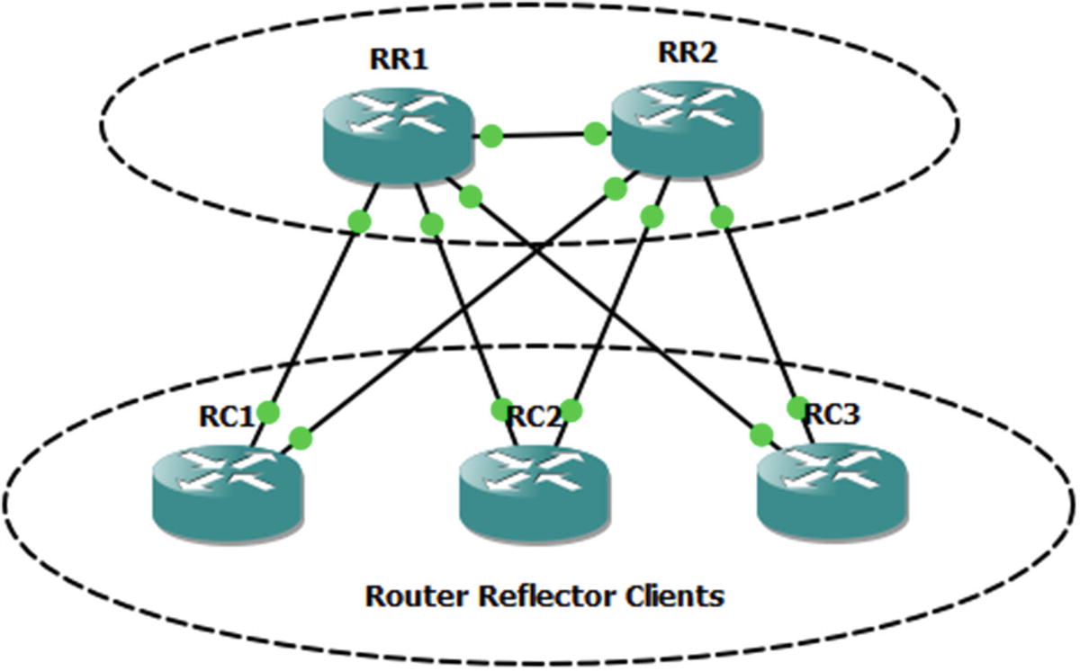
Router reflection
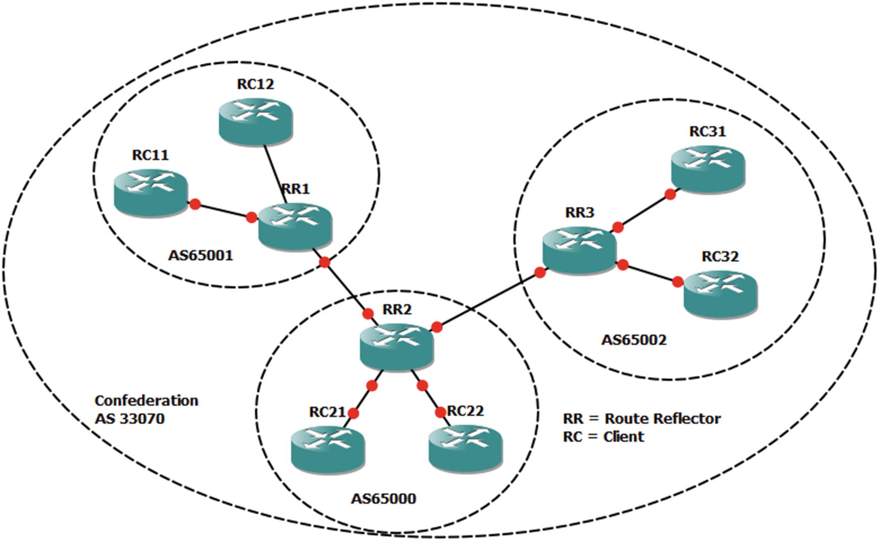
Reflectors and confederations
BGP Decision Process
Metric | Preferred Choice |
|---|---|
Weight (Cisco proprietary) | Highest |
Local preference | Highest |
Origination | Local |
AS_PATH | Lowest |
Origin type | IGP, then EGP, then Incomplete |
MED | Lowest |
BGP type | eBGP |
IGP metric to next hop | Lowest |
Prefix age | Oldest |
Router ID | Lowest |
Cluster length | Lowest |
Neighbor address | Lowest |
Table 12-1 may seem like a lot, but it uses a top-down approach and stops once decision criteria are met. It is also important to note that many of the decisions are relevant to the direction. For example, local preference is used when administrators prefer a specific path out of their networks. The length of the autonomous system path can be manipulated by prepending your autonomous system to influence others to choose a certain path by making an alternate path longer.
The Multiple Exit Discriminator (MED) is often used when all else is equal. The MED is a hint to external peers about which path they should prefer. It is often determined by the metric from the IGP. By default, the MED is compared when the AS PATH is the same length and the first autonomous system in the path is the same. However, it can be configured to not require the same first autonomous system. It also has some issues with missing MEDs. By default, a missing MED has a value of 0, which is considered best. To fix this issue, the command bgp bestpath med missing-as-worst reverses the behavior.
Once BGP makes the decision about which prefix it wants to put in the routing table, you could have problems if you actually want an IGP to win. Think about the case where tunnel endpoints are learned through an IGP; but when the tunnel comes up, they get advertised through eBGP as going through the tunnel. In this case, eBGP wins due to its administrative distance of 20. When a routing protocol claims that the tunnel endpoints are reachable through the tunnel, the tunnel flaps. In the case of BGP, this is an easy fix. When you want to advertise a network, but you want it to lose to IGPs, you advertise it as a backdoor network. This sets the administrative distance to 200, even when it is advertised to an external peer.
Similar to other protocols, BGP has built-in security features. One of them is a check on the receiving interface. BGP uses TCP and needs to make a connection using consistent addresses. With eBGP, this is usually not a problem because the links are frequently point to point. With iBGP, the peers may be connecting across a campus. In the case of iBGP, it is usually recommended to set the update source as a loopback interface and peer to that interface. In the case of eBGP, it is best to use the physical interface addresses. One reason is that eBGP has a security feature that restricts the TTL to 1. If an eBGP peer is not directly connected, you need to manually configure ebgp-multihop with the TTL on the neighbor statement. This feature shouldn’t be confused with TTL security, and they cannot be used together. Setting ttl-security on a neighbor works similarly as with OSPF TTL security. The hop count is subtracted from 255. BGP packets are sent out with a TTL of 255. If they have a TTL less than (255 – hop count), they are discarded.
Loopbacks provide a slightly different case than traditional multihop. By default, eBGP will not peer using loopback. You could set ebgp-multihop to 2 or ttl-security hops to 2, but with loopback, disable-connected-check on the eBGP neighbor is a more secure option. This option enforces the TTL of 1 to get to the peer, but it essentially won’t count the extra hop to the loopback. Just don’t forget to make the loopback reachable from the peer. You usually don’t use IGPs with eBGP peers, so they may need a static route to the loopback.
Protocol-Independent Multicasting
Protocol-Independent Multicasting (PIM) is a family of control plane protocols used for multicast routing. Multicast routing doesn’t have fixed endpoints like with unicast. It can have multiple hosts in different networks receiving a multicast stream. The protocols need to figure out the most efficient tree to build to get data from the sender to all of the receivers. It uses the unicast routing protocols and multicast messages from participating hosts to accomplish this.
The PIM variants are dense mode, sparse mode, bidirectional PIM, and Source-Specific Multicast (SSM ). Each variant builds trees for multicast groups, also known as multicast addresses, but they use different mechanisms.
PIM dense mode is used when the assumption is that there are multicast receivers at most locations. When PIM dense mode is in use, it builds trees for a multicast group to get to every participating router in the network. When a router doesn’t want to receive traffic for a multicast group, it sends a prune message. This is a simple-to-configure method, but it isn’t scalable and it can cause network degradation when there are several high-bandwidth multicast streams, in which most segments don’t want to participate.
PIM sparse mode operates on the opposite assumption of dense mode. Sparse mode assumes that most network segments don’t have multicast receivers. This can scale better over a WAN than dense mode. It uses rendezvous points (RPs) to help manage the trees. In large networks, there can be multiple RPs that share information, and RPs can be dynamically selected. In smaller networks, static RPs are often assigned. Even in large networks, a static address can be used for the RP, and unicast routing can provide the path to the closest active RP.

Sparse mode multicasting
When a multicast packet is sent out of an interface to receivers, it is translated to multicast frames. This layer 2 destination starts with 01:00:5E and then uses the 23 lowest-order bits from the layer 3 address. If the switch doesn’t know which ports are listening on a multicast group, it will send the frames to all of the ports, except the port on which the frames were received. This is where IGMP snooping comes in to play. The Internet Group Management Protocol (IGMP) is the protocol used by hosts to notify a router when they join and leave multicast groups. IGMP snooping is a protocol that allows layer 2 devices to peek at IGMP messages that pass through them and use the information to determine which switchports want multicast frames for particular groups. It is enabled by default, but can be disabled using the global command no ip igmp snooping. It can also be disabled on a per-VLAN basis, but if it is disabled globally, it cannot be enabled on a VLAN.
Before leaving the topic of the multicast control plane, we should point out an often problematic security feature for the multicast control plane: reverse path forwarding (RPF) checks. RPF checks use the unicast routing table to verify that the multicast source address is reachable through the interface where it received the packet. Problems can occur when PIM isn’t enabled on all the interfaces or there is some asymmetry to the routing. The quick fix when you receive RPF check failure messages is to use the ip mroute global configuration command to add a path to the multicast routing table. This, however, is often just a Band-Aid fix; and it doesn’t address the root of the problem. To properly fix the problem, you need to analyze your unicast routing to determine why it is failing the RPF checks.
Domain Name System
Network Time Protocol
The Network Time Protocol (NTP) is a protocol for synchronizing time between devices. Accurate—or least synchronized—time is important for the management of network devices. The basic functionality of routing and switching doesn’t require synchronized time, but it is important for management tasks such as analysis of log files. It is also important for use in security features, such as time-based access control lists and cryptologic key rotation.
NTP uses strata as a measure of the reliability of a time server. A device with a stratum value of 0 is considered to be the most accurate time source. Each NTP hop adds a stratum number until the maximum stratum value of 15. If a device tries to synchronize to a stratum 15 device, it will receive an error stating that the stratum is too high.
So far, only unrestricted NTP has been discussed. To add a layer of security, you can use access lists and authentication.
Peer: This allows all types of peering with time servers in the access list. Routers can synchronize with other devices and can be used as time servers.
Query-only: This restricts devices in the access list to only use control queries. Responses to NTP requests are not sent, and local time is not synchronized with time servers specified in the access list. No responses to NTP requests are sent, and no local system time synchronization with remote system is permitted.
Server: This allows the device to receive time requests and NTP control queries from the servers specified in the access list, but not to synchronize itself to the specified servers.
Server-only: This allows the router to respond to NTP requests only. It does not allow attempts to synchronize local system time.
Tools for Control Plane Management
We discussed the management plane in Chapter 10, but it is worth revisiting in terms of tools. Some software-defined networking architectures completely manage the control plane. The typical Cisco architecture is to allow each device to run control plane protocols, but we may configure parameters used by those protocols with tools.
Cisco Prime Infrastructure is a good choice when there is a mix of manual configuration and configuration pushed by the tool. Prime Infrastructure logs into the device and periodically pulls the configuration. This allows you to make changes from the current state of the device. It also allows Prime Infrastructure to validate compliance. If you want to get extremely fancy, you can even have Prime automatically run show commands and push configuration changes based on the result. However, that is not recommended unless you have extremely fine-tuned templates and have tested all your automatic configuration rules.
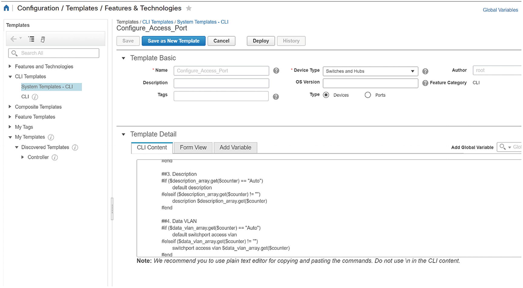
Access port template script

Template variables

Template form preview
In the following example, we inspect the current state of routing protocols in the managed routers. We then apply a template and validate that the changes have been made. Please note that the example provided here can be disruptive. It should not be used on a live network without testing. Our example is simple and does not use variables. It is intended to just give you an idea of how simple a template can be.
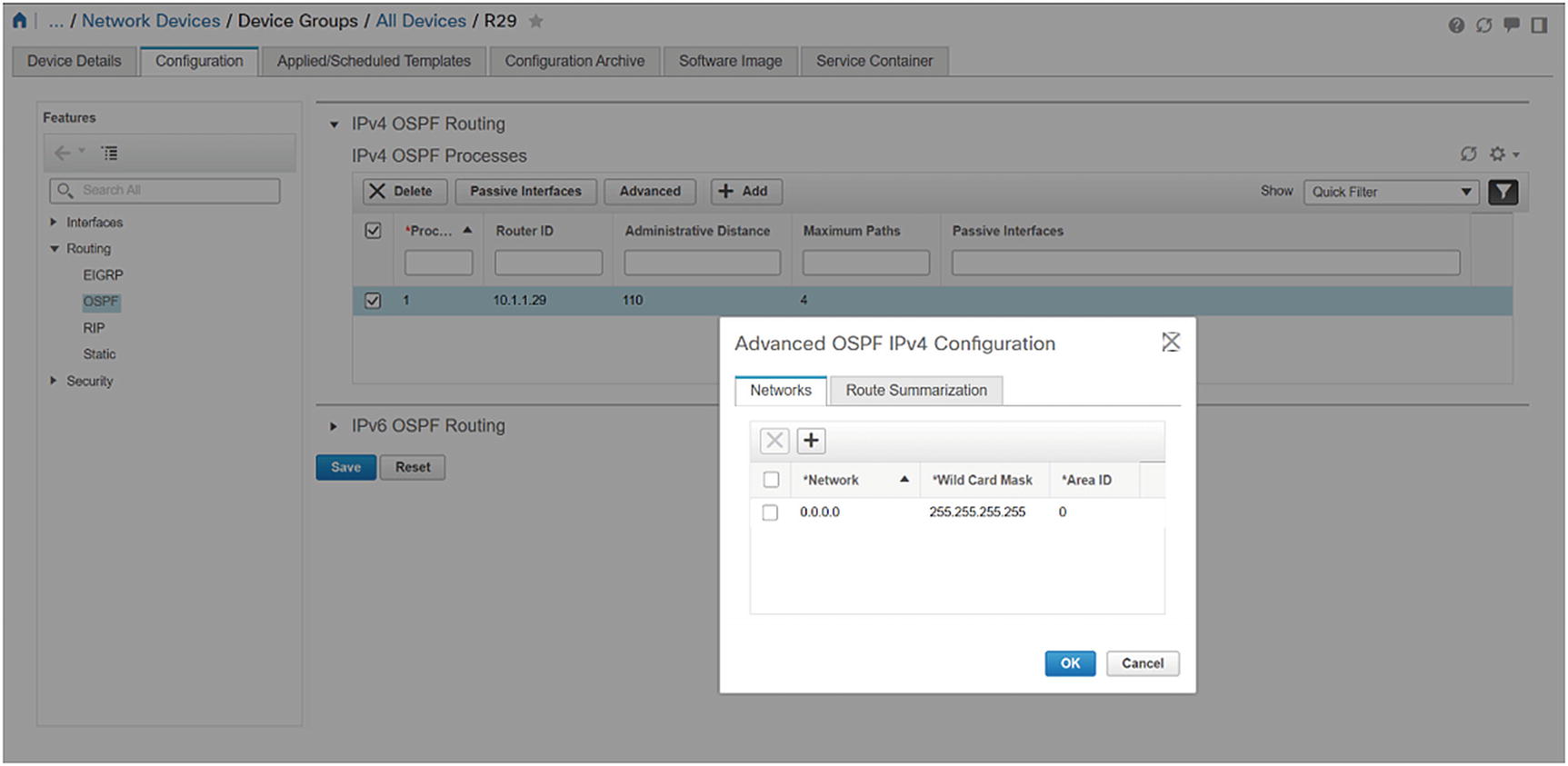
Router initial state

CLI template

Deploy the template
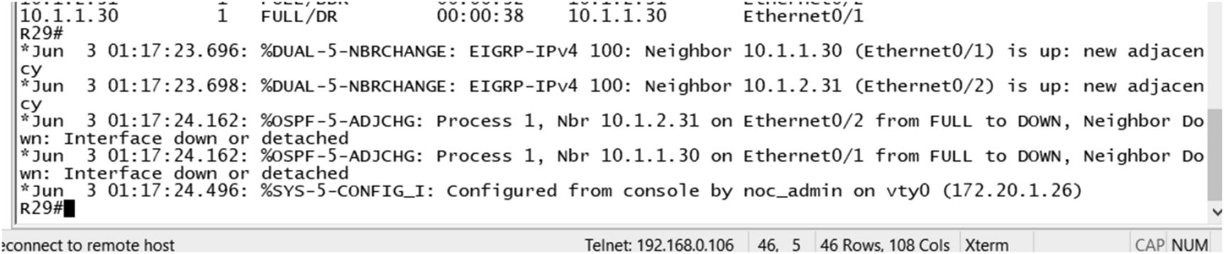
Console logs after template deployment
Exercises
The exercises in this section are cumulative. If you have problems with an exercise, use the answer to get to the end state before moving on to the next exercise.
Preliminary Work
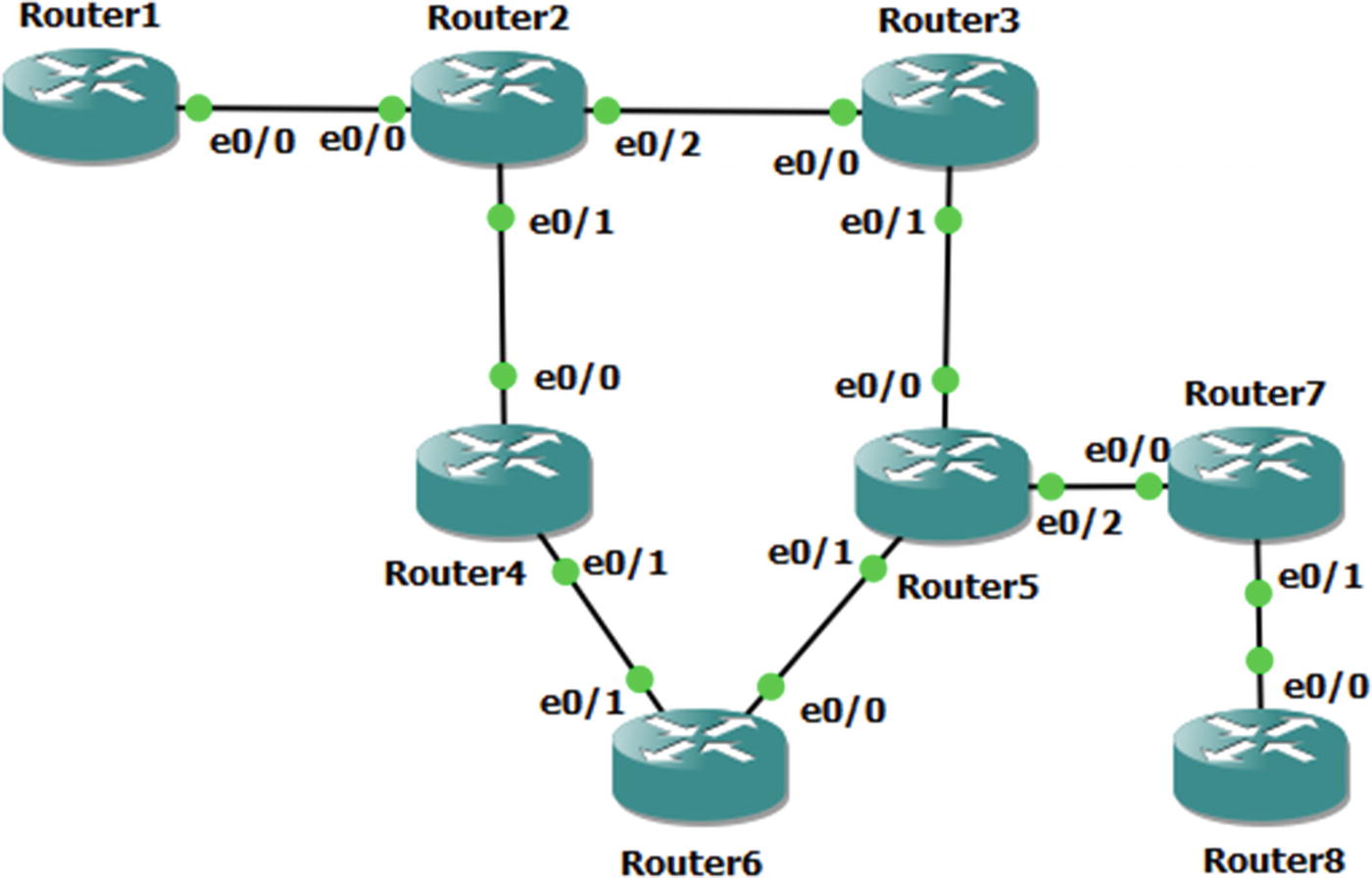
Exercise network typology
Router Interface Addresses
Router | Interface | Address |
|---|---|---|
Router1 | Ethernet0/0 | 192.168.12.1/24 |
Router1 | Loopback10 | 10.1.1.1/24 |
Router1 | Loopback172 | 172.16.1.1/32 |
Router2 | Ethernet0/0 | 192.168.12.2/24 |
Router2 | Ethernet0/1 | 192.168.24.2/24 |
Router2 | Ethernet0/2 | 192.168.23.2/24 |
Router2 | Loopback172 | 172.16.2.2/32 |
Router3 | Ethernet0/0 | 192.168.23.3/24 |
Router3 | Ethernet0/1 | 192.168.35.3/24 |
Router3 | Loopback172 | 172.16.3.3/24 |
Router4 | Ethernet0/0 | 192.168.24.4/24 |
Router4 | Ethernet0/1 | 192.168.46.4/24 |
Router4 | Loopback172 | 172.16.4.4./24 |
Router5 | Ethernet0/0 | 192.168.35.5/24 |
Router5 | Ethernet0/1 | 192.168.56.5/24 |
Router5 | Ethernet0/2 | 192.168.57.5/24 |
Router5 | Loopback172 | 172.16.5.5/32 |
Router6 | Ethernet0/0 | 192.168.56.6/24 |
Router6 | Ethernet0/1 | 192.168.46.6/24 |
Router6 | Loopback10 | 10.6.6.6/24 |
Router6 | Loopback172 | 172.16.6.6/32 |
Router7 | Ethernet0/0 | 192.168.57.7/24 |
Router7 | Ethernet0/1 | 192.168.78.7/24 |
Router7 | Loopback172 | 172.16.7.7/32 |
Router8 | Ethernet0/0 | 192.168.78.8/24 |
Router8 | Loopback10 | 10.8.8.8/24 |
Router8 | Loopback172 | 172.16.8.8/32 |
OSPF
OSPF Areas
Router | Interface | Area |
|---|---|---|
Router2 | Ethernet0/2 | Area 1 |
Router2 | Loopback172 | Area 1 |
Router2 | Ethernet0/1 | Area 2 |
Router3 | Ethernet0/0 | Area 1 |
Router3 | Loopback172 | Area 1 |
Router3 | Ethernet0/1 | Area 2 |
Router4 | Ethernet0/0 | Area 2 |
Router4 | Ethernet0/1 | Area 0 |
Router4 | Loopback172 | Area 0 |
Router5 | Ethernet0/0 | Area 2 |
Router5 | Ethernet0/1 | Area 0 |
Router5 | Loopback172 | Area 0 |
Router6 | Ethernet0/0 | Area 0 |
Router6 | Ethernet0/1 | Area 0 |
Router6 | Loopback172 | Area 0 |
Router6 | Loopback10 | Area 3 |
BGP
BGP Configuration Parameters
Router | Autonomous System | Advertised Networks |
|---|---|---|
Router1 | 65001 | 10.1.1.0 mask 255.255.255.0 192.168.12.0 |
Router2 | 65256 | 192.168.12.0 192.168.23.0 192.168.24.0 |
Router5 | 65256 | 192.168.35.0 192.168.56.0 192.168.57.0 |
Router6 | 65256 | 192.168.46.0 192.168.56.0 10.6.6.0 mask 255.255.255.0 |
Router7 | 65078 | 192.168.57.0 192.168.78.0 |
Router8 | 65078 | 192.168.78.0 10.8.8.0 mask 255.255.255.0 |
Router1 and Router2
Router2 and Router5
Router5 and Router6
Router5 and Router7
Router7 and Router8
Verify routing to all Ethernet interfaces and Loopback10 interfaces.
NTP
Configure Router2 as a stratum 3 time source. Configure Router3, Router4, Router5, and Router6 as clients. Use Loopback172 interfaces for NTP. Use an authentication key of “Apress.”
Named Mode EIGRP with Authentication
You are already running OSPF. You will run EIGRP on top of it. Since EIGRP has a better administrative distance than OSPF, you should see that networks are learned over EIGRP instead of OSPF.
- 1.
On each router, create a key with a send and receive lifetime of January 1, 2015, through December 31, 2030. Use “Apress” as the key.
- 2.
Create a named mode EIGRP instance.
- 3.
Use autonomous system 10.
- 4.
Configure EIGRP to advertise any networks in 192.0.0.0/8.
- 5.
Enable authentication and reference the key that you pre-staged.
Multicast
Configure Loopback172 on Router6 as a listener for multicast group 229.1.1.1.
Configure the multicast domain such that a sender on Router2 can take any path to get to the listener on Router6. Use a technique that will assume that most router segments will have listeners.
Exercise Answers
This section contains the solutions to the exercises. Overview explanations are provided for each solution.
Preliminary Configurations
The preliminary configurations contain the snippets required to start working on the exercises. This section addresses the interfaces and creates the necessary loopback interfaces.
Configuration Snippets
Verification
OSPF
The purpose of this exercise is to demonstrate the use of virtual links. When you configure the areas per the table, you attempt to transit a non-backbone area. To fix this, you need to create a virtual link. A virtual link between either Router2 and Router4 or Router3 and Router5 will fix the problem. For redundancy, you created a virtual link for each path.
Configuration Snippets
Verification
BGP
There are two potential pitfalls in this exercise. One of them is that there isn’t a full mesh for the iBGP peers in AS 65256. Either a confederation or route reflection would work. In this case, route reflection makes more sense.
Configuration Snippets
Verification
NTP
The configuration of NTP is mostly straightforward, but can be prone to error. The configuration is identical on each client, as they all point to the same NTP server.
One issue that can cause concern when configuring NTP is that it can take time for time sources to synchronize. Don’t be concerned if associations don’t immediately reflect that they are synchronized; however, if a substantial amount of time passes and there still isn’t a synchronized association, you need to start troubleshooting.
Configuration Snippets
Verification
Named Mode EIGRP with Authentication
The main purpose of this exercise was to experiment with EIGRP in named mode. This style of configuring EIGRP pulls all of the configuration into the EIGRP process and allows for configuration of multiple address families.
In this exercise, you used MD5 authentication with a key chain. The key chain provides the ability to easily change keys. Another option with named mode EIGRP is to use SHA256, but as of IOS 15.4, that method does not allow the use of key chains.
Configuration Snippets
Verification
Multicast
A key to this exercise is that most segments will have listeners. This makes PIM dense mode the best choice.
If you look at unicast routing, you see that the best path is through Router4, but you want it to work for any path. If Router4 is not available or not selected for some reason, you need to be able to go through Router3 and Router5 to get to Router6.
Configuration Snippets
Verification
Summary
This chapter provided a review of protocols, but added new information and theory about the protocols as they pertain to the control plane. It also introduced a few additional control plane protocols, such as PIM, DNS, and NTP.
The next chapter tightens the focus as you delve into availability.